Research on Multi-Objective Optimization and Control Algorithms for Automatic Train Operation

Abstract

The automatic train operation (ATO) system of urban rail trains includes a two-layer control structure: upper-layer control and lower-layer control. The upper-layer control is to optimize the target speed curve of ATO, and the lower-layer control is the tracking by the urban rail train of the optimal target speed curve generated by the upper-layer control according to the tracking control strategy of ATO. For upper-layer control, the multi-objective model of urban rail train operation is firstly built with energy consumption, comfort, stopping accuracy, and punctuality as optimization indexes, and the entropy weight method is adopted to solve the weight coefficient of each index. Then, genetic algorithm (GA) is used to optimize the model to obtain an optimal target speed curve. In addition, an improved genetic algorithm (IGA) based on directional mutation and gene modification is proposed to improve the convergence speed and optimization effect of the algorithm. The stopping and speed constraints are added into the fitness function in the form of penalty function. For the lower-layer control, the predictive speed controller is designed according to the predictive control principle to track the target speed curve accurately. Since the inflection point area of the target speed curve is difficult to track, the softness factor in the predictive model needs to be adjusted online to improve the control accuracy of the speed. For this paper, we mainly improve the optimization and control algorithms in the upper and lower level controls of ATO. The results show that the speed controller based on predictive control algorithm has better control effect than that based on the PID control algorithm, which can meet the requirements of various performance indexes. Thus, the feasibility of predictive control algorithm in an ATO system is also verified.

1. Introduction

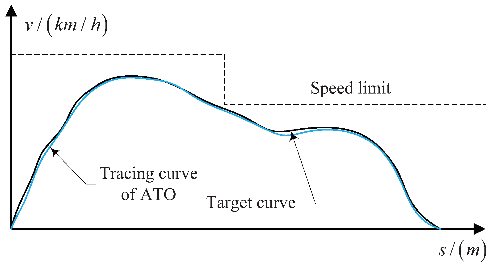
Since the urban rail train can carry more passengers and has higher comfort and safety, it has become the key development object of rail transit [1,2]. At this stage, the urban rail train mainly uses manual driving mode in the world [3]. Although the traditional manual driving mode has its own advantages, the development of automatic train operation (ATO) is an inevitable trend. For the traditional manual driving mode, the driver is prone to fatigue driving, thus reducing the driving efficiency of the train. With the continuous improvement of the performance requirements for urban railway train, the manual driving mode has been unable to meet the operational requirements of train and has gradually shown its own shortcomings. Therefore, ATO system has been developed rapidly due to its rapidity, punctuality, and safety [4,5,6]. The ATO system can adjust the traction or braking forces of the train in real time according to the operating conditions so that it can run safely and efficiently [7]. The typical ATO system includes a two-layer control structure. For the upper-layer control comprehensively considering the stopping accuracy index, punctuality index, comfort index, and energy consumption index, the ATO system calculates the optimal target speed curve according to the sensor information (speed, position, slope, etc.). For the lower-layer control, ATO system gives control instructions according to the tracking control strategy to make the train track the optimal target speed curve obtained by upper-layer control. In short, the core task of the ATO control system is to adjust the running speed of the train, as shown in Figure 1.

In Figure 1, the ATO speed controller controls the train according to the feedback information of the sensor so that the actual running speed tracks the target speed (see Figure 2).

The target speed curve with the best performance indexes is the important theoretical basis for speed tracking control. Taking into account multiple performance indexes such as safety, energy consumption, comfort, stopping accuracy, and punctuality, many scholars have optimized the target speed curve (also called the reference trajectory) of the train through different intelligent optimization algorithms. Rong et al. [8] formulated the multi-objective optimization model of urban rail train with energy saving, punctuality, and accurate stopping as optimization goals. The model is solved by particle swarm optimization (PSO), and a method to improve the acceleration coefficient of PSO is proposed. The improved algorithm can obtain more accurate global optimal values, that is, the optimal target speed curve. Liang et al. [9] used genetic algorithm (GA) to optimize the multi-objective optimization model of the train from five aspects: safety, stopping accuracy, punctuality, energy consumption, and comfort. In order to obtain the more accurate target speed curve of ATO, the penalty function is put into the objective function to improve GA. Zhao et al. [10] described a study on the optimization of the train driving curve to consider the trade-off between reductions in train energy usage against increases in delay penalties in a delay situation. Three search methods, namely, enhanced brute force, ant colony optimization, and GA, are used to quickly find the optimal operating curve and driving mode. Gu et al. [11] presented a new energy-efficiency train operation model based on real-time traffic information through the nonlinear programming method. More specifically, an energy-efficiency operation model is established based on trajectory analysis when the optimal energy-efficiency control is applied, from which an energy-efficiency reference trajectory is obtained under the constraints of running time and distance. Lu et al. [12] used two strategies to obtain the energy-efficient trajectory of the single train. One is to allow the train to coast, thereby using its available time margin to save energy. The other one is to dynamically control the speed while maintaining the required travel time. In addition, the train trajectory searching model based on distance is also proposed and the optimal speed trajectory of the train is searched by an ant colony optimization algorithm. Based on the research results of References [8,9,10,11,12], in this paper, the multi-objective model of urban rail train operation is firstly built with energy consumption, comfort, stopping accuracy, and punctuality as optimization indexes and an IGA based on directional mutation [13] and gene modification is proposed to search the optimal target speed curve. Moreover, the stopping and speed constraints are added into the fitness function in the form of penalty function [14,15]. IGA makes up for the shortcomings of traditional GA, such as slow convergence rate and poor optimization effect.

Tracking control algorithm of target speed curve is the second important problem in ATO system research [16,17]. The actual speed needs to be constantly adjusted in the operating process of the train to make it track the target speed curve closely, so the requirement of the control performance for the speed controller is very high [18]. With the continuous improvement and maturity of intelligent control algorithms, the speed control method of urban rail trains is also constantly improving. Cao et al. [19] designed the fuzzy predictive controller for speed tracking of ATO based on fuzzy logic and predictive control. The results show that the fuzzy predictive controller can significantly improve the safety, comfort, and stopping accuracy of trains. Chang et al. [20] proposed a new differential evolution method based on Pareto-optimal set to optimize the fuzzy controller of ATO. The multi-objective optimization method based on Pareto optima can provide a set of optimal nondominant solutions for decision makers. The optimized fuzzy controller can achieve well the control effect of speed tracking. Gao et al. [21] proposed a robust adaptive control method for the ATO system, which explicitly considers the actuator saturation nonlinearity besides unknown system parameters. Simulation results show that this method can achieve accurate speed tracking control. Shen et al. [22] adopted fuzzy control algorithm in combination with the PID control algorithm to control the ATO system of urban rail transit, which makes up the deficiency of traditional PID control algorithm, with the intention of achieving accurate speed tracking control. Although the literature [19,20,21,22] mainly studies lower-layer control, they all implement speed tracking on the basis of upper-layer control. Therefore, they also have successfully implemented two-layer control. Based on the above research results, the predictive speed controller is designed according to the predictive control principle to track the target speed curve accurately. Because there are many categories of predictive control, the dynamic matrix control (DMC) is used in this paper [23,24,25]. DMC directly takes the discrete coefficient of the step response of the object as the model, thus avoiding parameter identification for the transfer function model or the state space equation model. Since DMC uses multistep estimation technology, it can effectively solve the problem of delay process. However, as the inflection point area of the target speed curve is difficult to track, we improve the basic DMC. The softness factor in the predictive model of DMC should be adjusted online to improve the control accuracy of the speed. Simulation results show that the improved dynamic matrix control (IDMC) has higher tracking control accuracy than the PID algorithm and that the multiple performance indexes obtained by IDMC such as energy consumption, comfort, stopping accuracy and punctuality have been also improved.

The rest of this paper is structured as follows: Section 2 describes the optimization of target speed curve for urban rail trains. Section 3 presents the design of speed controller based on predictive control for urban rail trains. Section 4 discusses the experimental results. Finally, conclusions and outlooks are given in Section 5.

2. Optimization of Target Speed Curve for Urban Rail Train

The ideal target speed curve of an urban rail train is the reference input of an ATO speed controller. In the operating process of the train, different operating conditions can produce different speed curves. In this paper, based on energy consumption, comfort, stopping accuracy, and punctuality, the multi-objective optimization model of urban rail train is built. It is optimized by IGA to obtain an optimal target speed curve.

2.1. Force Analysis of Urban Rail Train

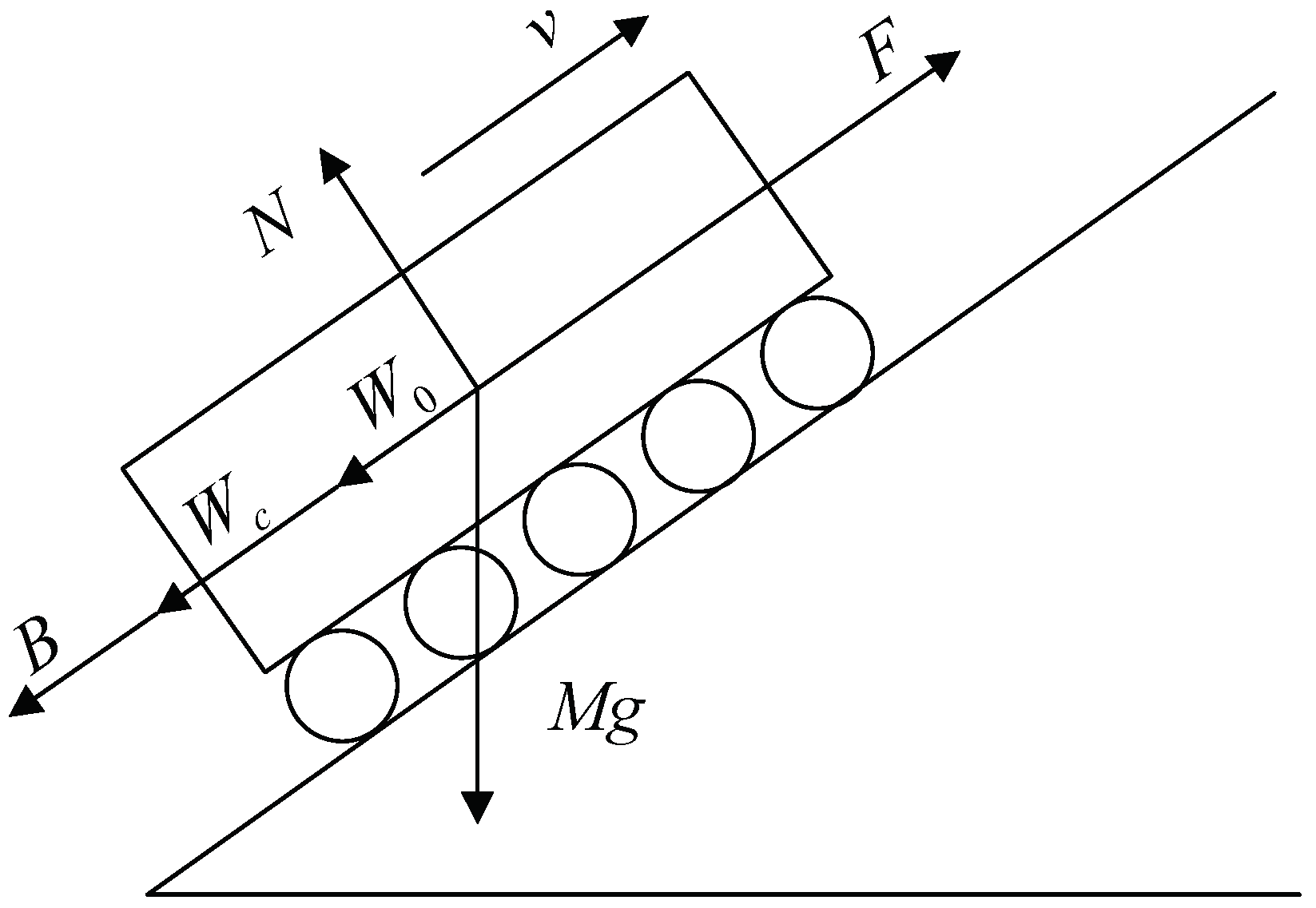
The urban railway train is mainly affected by traction, resistance, and braking forces in the operating process, as shown in Figure 3.

In Figure 3, the traction force F mainly provides the power for the train; the running resistance W includes basic resistance $W_0$ and additional resistance $W_c$; the braking force B is the force opposite to speed. It is not only used to slow down and stop but also to maintain a constant speed when the train is on a steep downhill.

2.1.1. Traction and Braking Forces

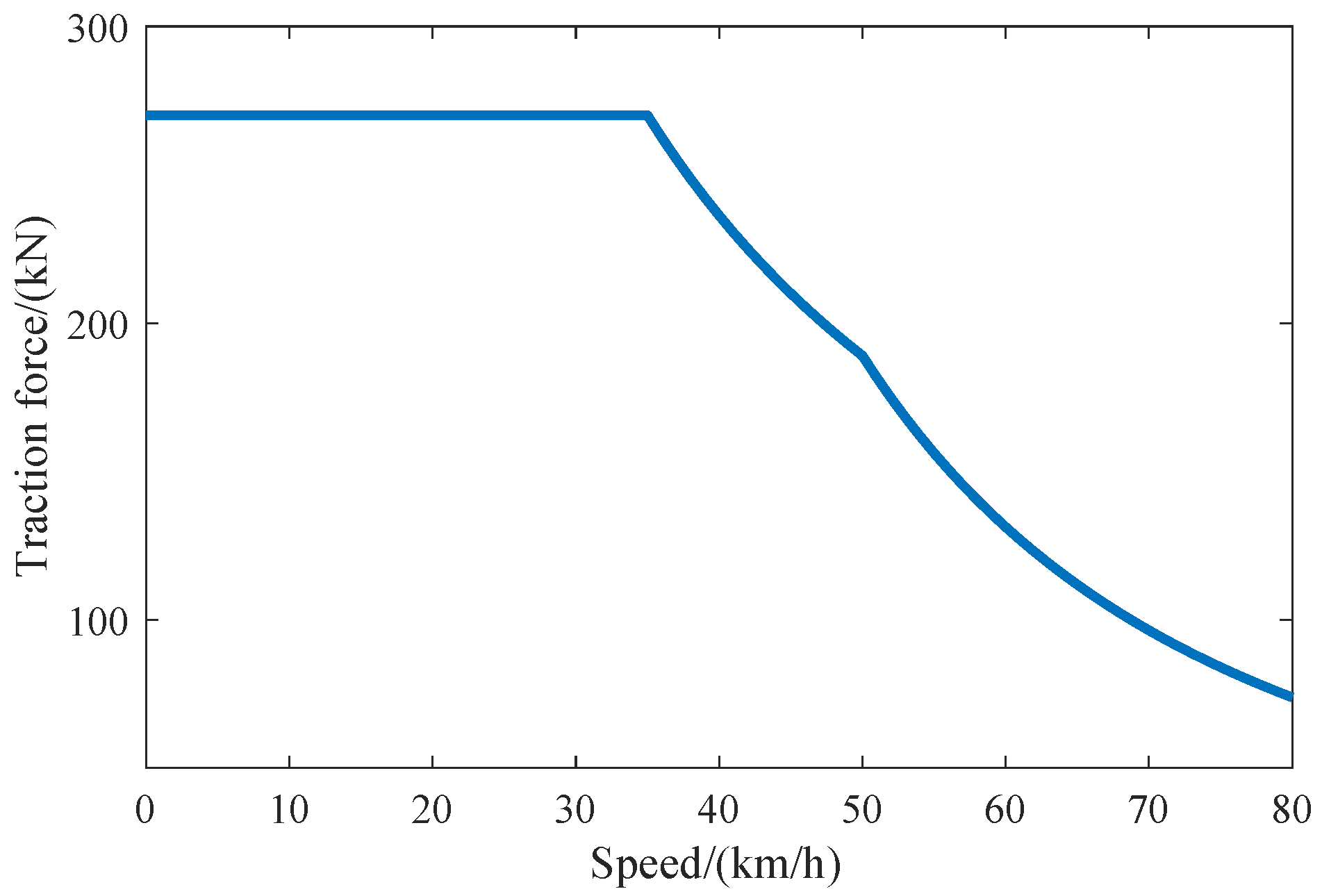
The traction system of urban rail train generally adopts stepless speed control, and the traction can be adjusted by the handle of the train. In addition, the traction characteristic curve of urban rail train reflects the relationship between the speed and traction force and each traction force has a corresponding speed value, as shown in Figure 4.

The air–electric blended braking is usually used to generate braking force for urban rail trains. After the train sends the deceleration signal, the electric brake is used first. If the electric brake cannot meet the train’s requirement for deceleration, the air brake will be used to supplement it. The electric braking force curve of urban rail train is shown in Figure 5.

2.1.2. Running Resistance

The running resistance W includes basic resistance $W_0$ and additional resistance $W_c$.

(1) Basic Resistance $W_0$

The basic resistance of the train mainly includes air resistance and friction on track. It is very difficult to calculate the specific basic resistance, so the unit basic resistance $w_0$ can be obtained according to the empirical equation of Equation (1).

$$w_0={\alpha }_1+{\alpha }_{2}v+{\alpha }_3{v}^2$$

(1)

where the unit of $w_0$ is N/kN; v is the actual speed of the train, the unit of which is km/h; ${\alpha }_1$ is the rolling resistance coefficient of the train; ${\alpha }_2$ is the mechanical resistance coefficient of the train; and ${\alpha }_3$ is the external air resistance coefficient of the train.

(2) Additional Resistance $W_c$

The additional resistance of urban rail train has nothing to do with its own attributes, and it is determined by the environment of the line, which mainly includes curve resistance, tunnel resistance, and ramp resistance.

• Curve Resistance
  When the train runs on the curve, it will encounter additional resistance from the curve. This curve resistance is related to the radius of the curve, the speed of the train, the bending degree of the track, and other factors. Therefore, it is difficult to get accurate results by using general mathematical methods. In this paper, according to experience, the unit curve resistance $w_r$ of the train is set to

  $$w_r=\frac{600g}{R}$$

  (2)

  where the unit of $w_r$ is N/kN; R is the radius of the curve, the unit of which is m; and g is the gravitational acceleration, the unit of which is m/s${}^2$.
• Tunnel Resistance
  When the train enters the tunnel, due to the existence of air, there is the pressure difference between the positive pressure on the head of the train and the negative pressure on the tail, which will create resistance to the train. The empirical equation of unit tunnel resistance $w_s$ can be expressed as follows.

  $$w_s=0.00013l_s$$

  (3)

  where the unit of $w_s$ is N/kN and $l_s$ is the length of the tunnel, the unit of which is m.
• Ramp Resistance
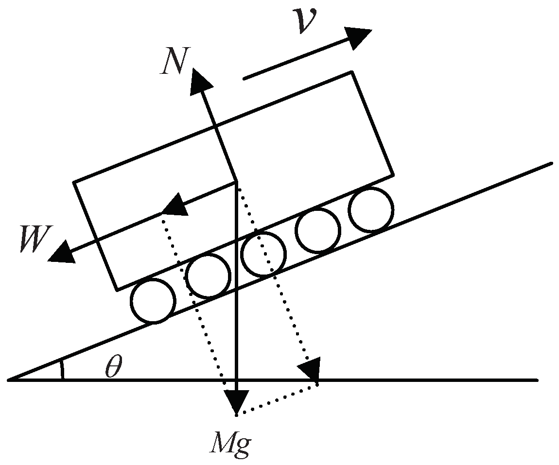
  When the train is running on the ramp, its gravity can generate the component force parallel to the track, that is, the ramp resistance. For uphill, the ramp resistance is opposite to the train’s running direction. For downhill, the ramp resistance is the same as the train’s running direction. The influencing factors of ramp resistance are related to the mass of train and ramp angle, as shown in Figure 6.
  According to Figure 6, the ramp resistance can be expressed as

  $${w_g}^{\prime }=Mgsin\theta$$

  (4)

  where ${w_g}^{\prime }$ is the ramp resistance of the train; M is the mass of the train; and $\theta$ is the angle between the level and the ramp.
  Since $\theta$ is very small in the actual line, we can approximate

  $$sin\theta =tan\theta =\theta$$

  (5)
  Therefore, the unit ramp resistance $w_g$ can be expressed as

  $$w_g=1000·sin\theta =\alpha$$

  (6)

  where $\alpha$ is the permillage of $\theta$ and the unit of $w_g$ is N/kN.

2.2. Multi-Objective Model of Urban Rail Train Operating Process

2.2.1. Establishment of Multi-Objective Model

The train operating process needs to consider multiple performance indexes such as energy consumption, comfort, stopping accuracy, and punctuality.

(1) Energy Consumption Index

The energy consumption of the train during its operation can be divided into three parts: traction energy consumption, auxiliary energy consumption, and regenerative braking energy. Therefore, in this paper, the energy consumption model of the train is established as follows.

$$En={\int }_0^S\left\{\frac{f\left(v\right)}{\eta }-\lambda \eta b\left(v\right)\right\}dx+AT$$

(7)

where E is the energy consumption model of the train; S is the actual running distance for the train between the two stations; f and b are the actual traction and braking forces of the train; $\lambda$ is regenerative braking energy utilization ratio, the range of which is from 0 to 1; T is the actual running time for the train between the two stations; A is the auxiliary power of the train; and $\eta$ is electromechanical efficiency of the whole train, of which its calculation formula is as follows.

$$\eta ={\eta }_{gear}·{\eta }_{\mathrm{cov}}·{\eta }_{motor}$$

(8)

where ${\eta }_{gear}$ is the transmission efficiency of the gear; ${\eta }_{\mathrm{cov}}$ is the efficiency of the converter; and ${\eta }_{motor}$ is motor efficiency.

(2) Comfort Index

Comfort is mainly affected by the acceleration and the acceleration change of train. In order to ensure that passengers feel comfort, the acceleration range is controlled between −1.4 m/s${}^2$ and 1.4 m/s${}^2$. The comfort model of the train is built as follows.

$$Co={\int }_0^T\left|\frac{da}{dt}\right|dt=\sum _{i=1}^n\left|a_{i+1}-a_i\right|$$

(9)

where a is the acceleration of the train; $a_i$ and $a_{i+1}$ are the accelerations at the ith sample point and at the $i+1$th sample point; and $\frac{da}{dt}$ is the rate of change of acceleration, also called $Jerk$.

In addition, we also consider the comfort evaluation table (see

Table 1. The comfort evaluation.

Jerk	Comfort Level
$\left|\Delta a\right|$ < 4.2 m/s${}^3$	Very comfortable
4.2 m/s${}^3$ $\le \left|\Delta a\right|$ < 7.5 m/s${}^3$	General comfortable
7.5 m/s${}^3$ $\le \left|\Delta a\right|$ < 13.4 m/s${}^3$	Not comfortable
13.4 m/s${}^3$ $\le \left|\Delta a\right|$	Very uncomfortable

) to evaluate the comfort level.

Therefore, $jerk$ cannot exceed 7.5 m/s${}^3$.

(3) Stopping Accuracy Index

For the current urban rail transit, most stations are equipped with a screen door system, which requires ATO to achieve accurate stopping. In order to ensure that passengers can get on and off the train normally, the stopping error is generally required to be within 30 cm. The stopping error accuracy model of the train is built as follows.

$$Pa=\left|S-S^{\prime }\right|$$

(10)

where S is the actual running distance of the train and $S\prime$ is the distance between two stations.

(4) Punctuality Index

The difference between the actual arrival time and the required arrival time of train is the important basis for the evaluation of punctuality. In general, the difference between the actual arrival time and the required arrival time should be less than 5% as far as possible. The punctuality model of the train is built as follows.

$$Pu=\left|T_{required}-T\right|$$

(11)

where $T_{required}$ is the required arrival time between two stations.

According to energy consumption, comfort, stopping error accuracy, and punctuality, the multi-objective optimization model of train is established as follows.

$$G=min\left\{En,Co,Pa,Pu\right\}$$

(12)

where G denotes that each sub-objective function should be minimized.

Since the operating process of an urban rail train is a multi-objective optimization problem, this paper uses the linear weighted method [26,27] to comprehensively take into account multiple performance indexes, thus transforming the multi-objective optimization problem into a single-objective optimization problem. Therefore, Equation (12) is converted to

$$G_Z={\omega }_{1}En+{\omega }_{2}Co+{\omega }_{3}Pu+{\omega }_{4}Pa$$

(13)

where ${\omega }_1$, ${\omega }_2$, ${\omega }_3$ and ${\omega }_4$ are weight coefficients, which satisfy ${\omega }_1+{\omega }_2+{\omega }_3+{\omega }_4=1$.

2.2.2. Weight Coefficient Calculation Based on Entropy Weight Method

Entropy weight method [28,29] is an objective weight coefficient distribution method, which mainly determines the weight coefficient through the change level of each index. Firstly, on the basis of judging the degree of difference among each index, the entropy weight of each index is calculated according to the information entropy [30]. Then, the entropy weight of each index is used to weigh all indexes.

For the evaluation system with m indexes and n evaluated objects, the normalized evaluation matrix $R_{n\times m}$ can be obtained by deducing the initial evaluation matrix $D_{n\times m}$ as follows.

$$D_{n\times m}=\left[\begin{array}{cccc}{D}_{11}& D_{12}& \cdots & D_{1m}\\ D_{21}& D_{22}& \cdots & D_{2m}\\ \cdots & \cdots & \cdots & \cdots \\ D_{n1}& D_{n2}& \cdots & D_{nm}\end{array}\right]\stackrel{R_{ij}=\frac{D_{ij}-\underset{i}{min\left(D_{ij}\right)}}{\underset{i}{max\left(D_{ij}\right)}-\underset{i}{min\left(D_{ij}\right)}}}{\to }{R}_{n\times m}=\left[\begin{array}{cccc}{R}_{11}& R_{12}& \cdots & R_{1m}\\ R_{21}& R_{22}& \cdots & R_{2m}\\ \cdots & \cdots & \cdots & \cdots \\ R_{n1}& R_{n2}& \cdots & R_{nm}\end{array}\right]$$

(14)

According to the theory of entropy weight method, the information entropy of the jth index can be obtained by Equation (15) and the entropy weight of the jth index can be obtained by Equation (16).

$$H_j=-\frac{1}{lnn}\sum _{i=1}^n{f}_{ij}ln{f}_{ij},\begin{array}{c}\end{array}{f}_{ij}=\frac{R_{ij}}{{\displaystyle \sum _{i=1}^n}{R}_{ij}},\begin{array}{c}\end{array}\left(j=1,2,\cdots ,m\right)$$

(15)

$${\omega }_j=\frac{1-H_j}{m-{\displaystyle \sum _{j=1}^m}{H}_j},\begin{array}{c}\end{array}\left(j=1,2,\cdots ,m\right)$$

(16)

where $0<{\omega }_j<1$, which satisfies ${\displaystyle \sum _{j=1}^m}{\omega }_j=1$. If $f_{ij}=0$, $f_{ij}ln{f}_{ij}=0$.

In this paper, there are 4 indexes ($En,Co,Pa$, and $Pu$) for the multi-objective problem of urban rail train and we choose 10 objects. Through the entropy weight method, the weight coefficients of $En,Co,Pa$, and $Pu$ can be obtained as 0.4121, 0.2981, 0.1901, and 0.0997, respectively.

2.3. Train Operation Strategy Optimization Based on IGA

For the train operation strategy optimization, an appropriate algorithm is needed to solve the multi-objective model of ATO to obtain the target speed curve. GA is the most widely used intelligent optimization algorithm in solving multi-objective optimization problems, so GA is chosen to solve the multi-objective model of urban rail train in this paper [31]. GA is a heuristic search algorithm which imitates the process of genetic selection in biological world through Darwin’s theory of natural selection [32,33]. In order to improve the optimization effect, the traditional GA is improved by combining directional mutation and gene modification. The IGA for train operation strategy optimization is described below.

2.3.1. Code Design

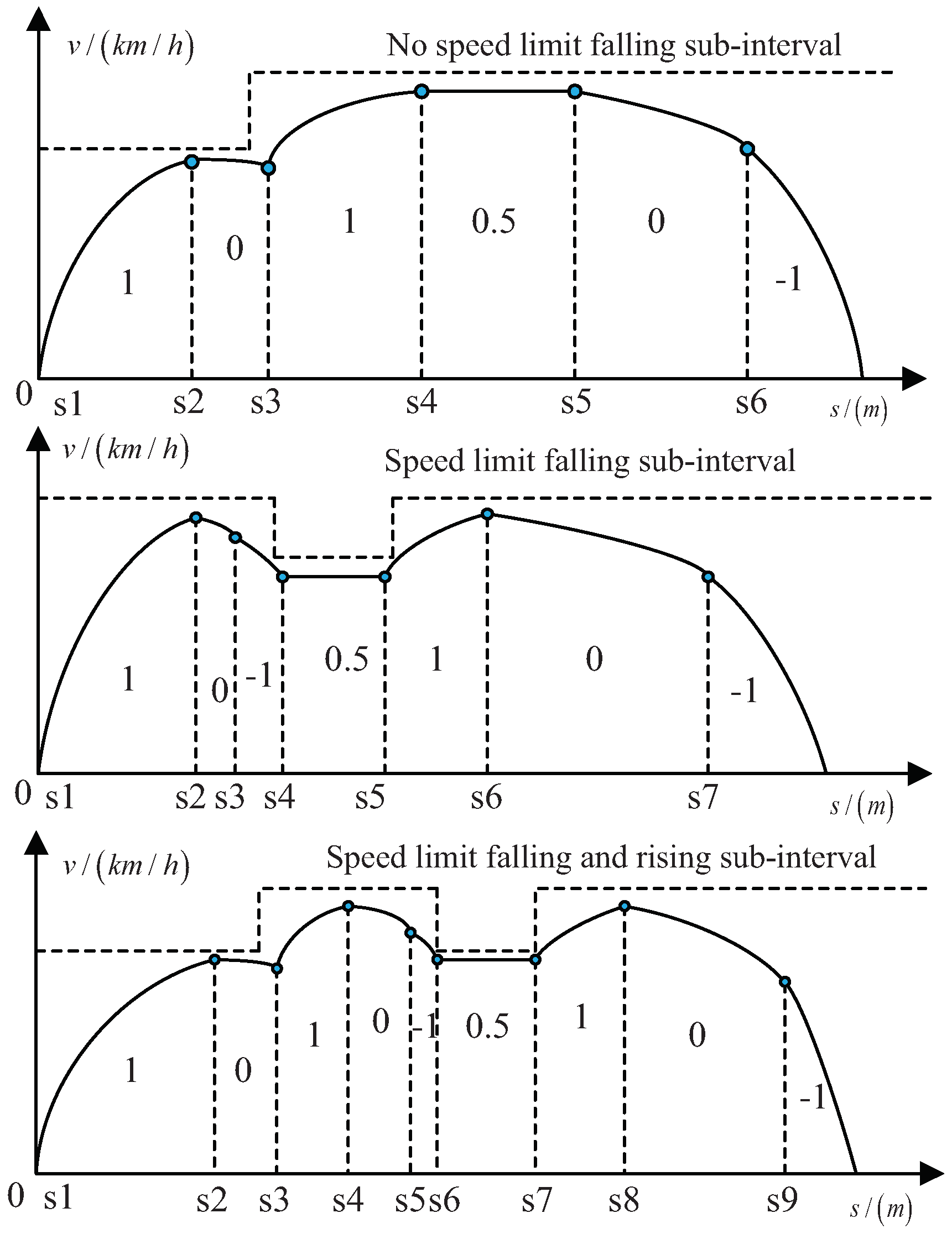
Coding is to transform the solution space of the problem into the search space that GA can handle. For the multi-objective optimization problem of urban rail train, the search space is so large; therefore, the real coding is adopted in this paper. Real coding omits the process of individual decoding and avoids the conversion of data type. Before coding, we first need to determine the number of variables of the solution. According to the driver’s experience, the smaller the number of train coasting, the lower the energy consumption. Therefore, the speed limit interval is divided into three speed limit subintervals, which are respectively the no-speed-limit falling subinterval, the speed-limit-falling subinterval, and the speed-limit-falling and rising subinterval. According to the driver’s experience, these three subintervals are designed as follows. In Figure 7, $\left\{1,0.5,0,-1\right\}$ respectively represent full traction condition, constant speed condition, coasting condition, and full braking condition. Here, full braking condition means that the train has applied maximum (electrical + pneumatic) braking force to braking. In addition, when the train is on a steep downhill, if the ramp resistance is greater than the running resistance, the speed of the train will increase during a coasting period. For these three subintervals, the encoding forms of their solutions (train operation strategies) are

$$\left\{\begin{array}{c}{U}_1=\left\{\left(s_1,1\right),\left(s_2,0\right),\left(s_3,1\right),\left(s_4,0.5\right),\left(s_5,0\right),\left(s_6,-1\right)\right\}\hfill \\ U_2=\left\{\left(s_1,1\right),\left(s_2,0\right)\right.\left.,\left(s_3,-1\right),\left(s_4,0.5\right),\left(s_5,1\right),\left(s_6,0\right),\left(s_7,-1\right)\right\}\hfill \\ U_3=\left\{\left(s_1,1\right),\left(s_2,0\right),\left(s_3,1\right),\left(s_4,0\right),(s_5,\right.\left.-1),\left(s_6,0.5\right),\left(s_7,1\right),\left(s_8,0\right),\left(s_9,-1\right)\right\}\hfill \end{array}\right.$$

(17)

where $U_1,U_2$, and $U_3$ are the train control sequences for the three speed limit subintervals; $(s_1,1)$ is a gene of $U_1$, in which 1 represents the full traction condition; and $s_1$ is the switching position of condition 1. Through these three typical subintervals, the coding design of the whole interval can be completed.

Moreover, on the basis of considering the constraint of speed, the influence of ramps on coding design is also considered. When the train is in a big downhill, the coasting condition (0) needed to be inserted in the corresponding position of the train control sequences $U_1$, $U_2$, and $U_3$, so that the train can make use of the gravitational potential energy as much as possible to save energy consumption.

2.3.2. Directional Mutation

GA mainly includes selection, crossover, and mutation operations. However, the traditional GA has slow convergence and lack of efficient mutation methods. Therefore, the mutation operation is improved in this paper. Since the gradient represents the direction where the function changes the most at a certain point, the gradient-based method can always converge at a faster speed. Therefore, the gradient information is introduced into GA to determine the mutation direction, so as to speed up the convergence rate of the algorithm and to improve the efficiency of the algorithm as follows.

For the optimization problem of finding the minimum value, it is defined as

$$miny=f\left(U\right)$$

(18)

where y is the target function and U is an individual in the population for GA as follows.

$$U={\left[u_1,u_2,\cdots ,u_n\right]}^T$$

(19)

Let us take two individuals $U_k,U_{k+1}$ in the population:

$$\left\{\begin{array}{c}{U}_k={\left[u_{k,1},u_{k,2},\cdots ,u_{k,n}\right]}^T\hfill \\ U_{k+1}={\left[u_{k+1,1},u_{k+1,2},\cdots ,u_{k+1,n}\right]}^T\hfill \end{array}\right.$$

(20)

Then, $y_k=f\left(U_k\right)$ and $y_{k+1}=f\left(U_{k+1}\right)$. Define the direction vector $d\left(U_{k+1},U_k\right)$:

$$d\left(U_{k+1},U_k\right)=\mathrm{sgn}\left(U_{k+1}-U_k\right)=\mathrm{sgn}\left(\left[u_{k+1,1}-u_{k,1},u_{k+1,2}-u_{k,2},\cdots ,u_{k+1,n}-u_{k,n}\right]\right)$$

(21)

When $y_{k+1}<y_k$, the vector $d\left(U_{k+1},U_k\right)$ is the evolution direction of from $U_k$ to $U_{k+1}$ and the opposite direction of $d\left(U_{k+1},U_k\right)$ is the degenerate direction.

If the target value is improved after directional mutation, the individual is retained; otherwise, it is discarded. In addition, the size of directional mutation decreases with the increase of iteration times as follows.

$$U_1=U_0+\left(1-\mathrm{ite}/\mathrm{it}{\mathrm{e}}_{max}\right)·d·rand$$

(22)

where $U_0$ is the individual before the directional mutation; $U_1$ is the individual after the directional mutation; $ite$ is the current number of iterations; ${\mathrm{ite}}_{max}$ is the maximum number of iterations; d is the direction vector; and $rand$ is a random number between 0 and 1.

2.3.3. Establishment of Fitness Function

The fitness function of GA is the only criterion of natural selection. The larger the fitness function value, the better. Since the train operation strategy optimization has several constraints such as speed limit and accurate stopping, the speed limit and stopping error are added to the objective function in the form of penalty function as follows.

$$Pe=a\underset{i}{\overset{n}{max}}{\left(max\left[0,\left(v_i-v_{imax}\right)\right]\right)}^2+b{\left(max\left[0,\left(\left|S-S^{\prime }\right|-0.3\right)\right]\right)}^2=P{e}_1+P{e}_2$$

(23)

where $Pe$ is the penalty function; $P{e}_1$ and $P{e}_2$ are the penalty terms of speed and stopping error, respectively; a and b are the weighting factors of the penalty function, which increase with the number of iterations; $v_i$ and $v_{imax}$ are the actual speed and limit speed of the train at the ith sample point; S is the actual running distance of the train two stations; and $S\prime$ is the distance between two stations. In order to ensure that passengers can get on and off the train normally, the stopping error is generally required to be within 30 cm.

Since the multi-objective optimization of train operation strategy is to find the minimum value, the fitness function is formed by taking the inverse of the sum of objective function and penalty function as follows.

$$fit=\frac{1}{G_{\mathrm{z}}+Pe}$$

(24)

where $G_{\mathrm{z}}$ is the objective function and $Pe$ is the penalty function.

2.3.4. Gene Modification

As there are many constraints involved in the train operation strategy optimization, the traditional GA is slow to seek the optimal solution and has low efficiency. Therefore, according to the driving experience, gene modification is carried out on chromosomes of which the penalty terms are not 0. Gene modification involves two cases as follows.

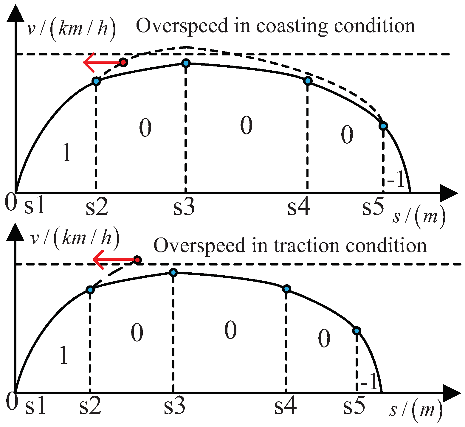
Case 1: The penalty term $P{e}_1$ of speed is not 0, as shown in Figure 8.

In Figure 8, the train overruns the speed limit in coasting condition “0” and traction condition “1” and the penalty term $P{e}_1$ of the speed is not 0. If the train still runs according to the original control strategy, it will endanger the safety. Therefore, the red traction points in Figure 8 should move appropriately to the left according to Equation (25).

$$s_2={s_2}^{\prime }-rand·L$$

(25)

where ${s_2}^{\prime }$ is the red traction point in Figure 8; $s_2$ is the modified traction point; $rand$ is a random number between 0 and 1; and L is the distance between ${s_2}^{\prime }$ and $s_1$.

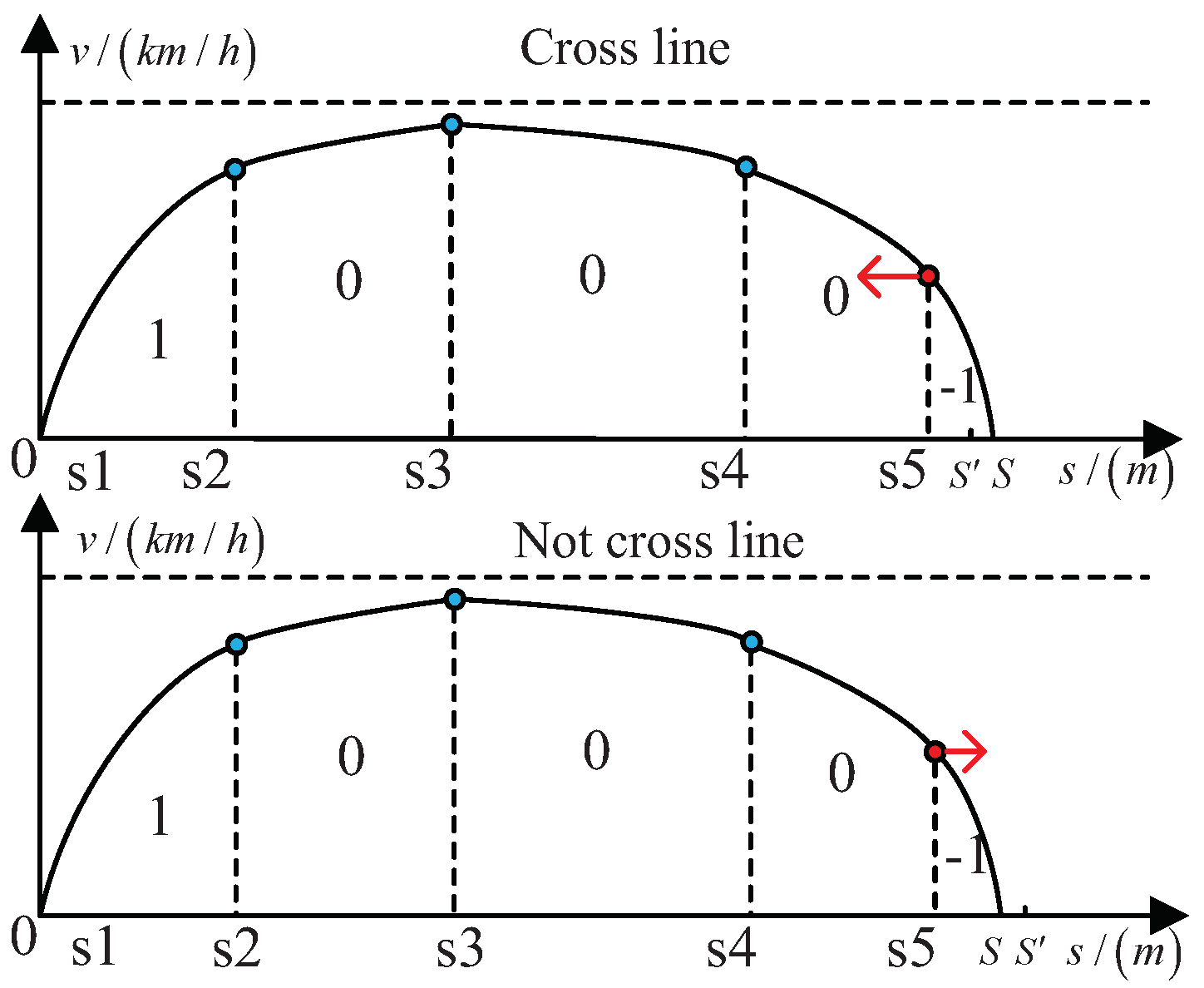
Case 2: The penalty term $P{e}_2$ of stopping error is not 0, as shown in Figure 9.

In Figure 9, S is the actual running distance of the train two stations and $S\prime$ is the distance between two stations. When S is larger than S’, the red braking point should be moved to the left appropriately according to Equation (26). When S is less than $S\prime$, the red braking point should be moved to the right appropriately according to Equation (27).

$${s_5}^{\prime }=s_5-L_1·rand$$

(26)

$${s_5}^{\prime }=s_5+L_2·rand$$

(27)

where $s_5$ is the red braking point in Figure 9; ${s_5}^{\prime }$ is the modified braking point; $L_1$ is the distance between $s_4$ and $s_5$; $L_2$ is the distance between $s_5$ and $S\prime$; and $rand$ is a random number between 0 and 1.

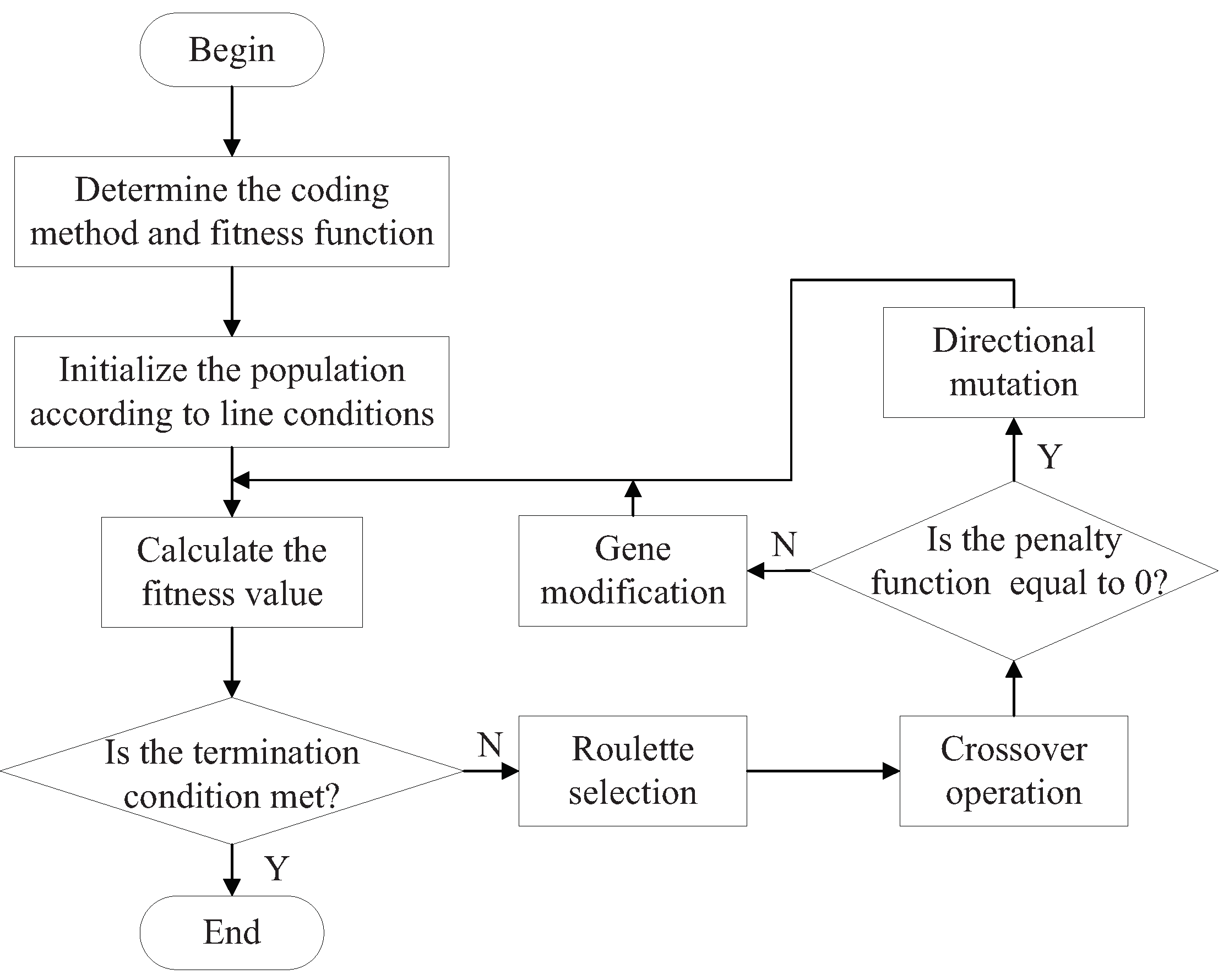
In conclusion, the flow chart of IGA is shown in Figure 10.

Moreover, an optimal operation strategy can be obtained by optimizing the multi-objective optimization model of urban rail train through IGA. Then, an optimal speed curve could be also obtained according to the optimal operation strategy, namely, the target speed curve.

3. Design of Speed Controller Based on Predictive Control for Urban Rail Train

There are many categories of predictive control, and this paper adopts DMC. DMC directly takes the discrete coefficient of the step response of the object as the model, thus avoiding parameter identification for the transfer function model or the state space equation model. Since DMC uses multi-step estimation technology, it can effectively solve the problem of delay process. DMC is also an optimal control technology, and it uses the quadratic performance index with the smallest deviation between the estimated output and the given value to implement control. The control structure of DMC mainly includes predictive model, rolling optimization, and feedback correction.

3.1. Predictive Model

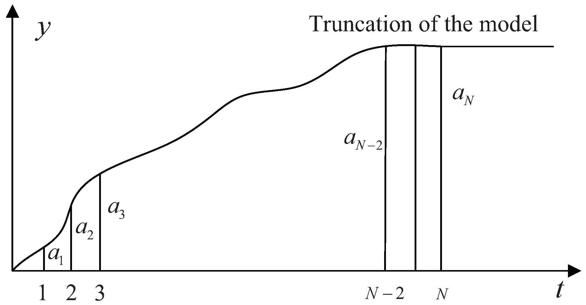
The dynamic performance of the controlled object can be described by a series of dynamic coefficients $a_1,a_2,\cdots ,a_N$, which are the values of the unit step response at the sample times. N is called the time domain length of the model (the truncation length of the model), and $a_N$ is the coefficient close enough to the steady-state value, as shown in Figure 11.

According to the model parameters $a_1,a_2,\cdots ,a_N$, the output values of the future moments for the controlled object can be predicted. When the control time domain M is greater than 1, there will be M continuous control increments $\Delta u\left(k\right),\Delta u\left(k+1\right),\cdots ,\Delta u\left(k+M-1\right)$. The predictive output ${\widehat{Y}}_M\left(k+1\right)$ of the system in the future prediction time domain P is as follows.

$${\widehat{Y}}_M\left(k+1\right)={\widehat{Y}}_0\left(k+1\right)+A\Delta U_M\left(k\right)$$

(28)

$$\Delta U_M\left(k\right)={\left[\begin{array}{cccc}\Delta u\left(k\right)& \Delta u\left(k+1\right)& \cdots & \Delta u\left(k+M-1\right)\end{array}\right]}^T$$

(29)

$${\widehat{Y}}_M\left(k+1\right)={\left[\begin{array}{cccc}\widehat{y}\left(k+1\right)& \widehat{y}\left(k+2\right)& \cdots & \widehat{y}\left(k+P\right)\end{array}\right]}^T$$

(30)

$${\widehat{Y}}_0\left(k+1\right)={\left[\begin{array}{cccc}{\widehat{y}}_0\left(k+1\right)& {\widehat{y}}_0\left(k+2\right)& \cdots & {\widehat{y}}_0\left(k+P\right)\end{array}\right]}^T$$

(31)

$$A=\left[\begin{array}{cccc}{a}_1& 0& \cdots & 0\\ a_2& a_1& \ddots & ⋮\\ ⋮& ⋮& \ddots & 0\\ a_M& a_{M-1}& \cdots & a_1\\ ⋮& ⋮& \cdots & ⋮\\ a_P& a_{P-1\cdots }& \cdots & a_{P-M+1}\end{array}\right]$$

(32)

where A is the dynamic matrix of DMC; P is the length of the time domain for the rolling optimization; and M is the length of the control time domain. In general, $N>P>M$.

3.2. Rolling Optimization

This paper uses DMC to make the closed-loop response of the system reach a new stable value along the target curve so as to improve the robustness of the system. Therefore, the input of the system is processed as follows.

$$w\left(k+j\right)={\alpha }^{j}y\left(k\right)+\left(1-{\alpha }^j\right)y_r$$

(33)

where $j=1,2,\cdots ,P$; $w\left(k+j\right)$ is the expected output value; $\alpha$ is the softness parameter ($0<\alpha <1$); $y\left(k\right)$ is the actual output value of the system; and $y_r$ is the given value of the system.

For DMC, the quadratic rolling optimization objective function is set to

$$\begin{array}{c}J=\sum _{j=1}^P{q}_j{\left[\widehat{y}\left(k+j\right)-w\left(k+j\right)\right]}^2+\sum _{j=1}^M{r}_j\Delta u^2\left(k+j-1\right)\hfill \\ ={\left[{\widehat{Y}}_P\left(k+1\right)-W_P\left(k+1\right)\right]}^{T}Q\left[{\widehat{Y}}_P\left(k+1\right)-W_P\left(k+1\right)\right]+\Delta {U_M}^T\left(k\right)R\Delta U_M\left(k\right)\hfill \\ ={∥{\widehat{Y}}_P\left(k+1\right)-W_P\left(k+1\right)∥}_Q^2+{∥\Delta U_M\left(k\right)∥}_R^2\hfill \end{array}$$

(34)

where $W_P\left(k+1\right)={\left[w\left(k+1\right),w\left(k+2\right),\cdots ,w\left(k+P\right)\right]}^T$; $Q=diag\left[q_1,q_2,\cdots ,q_P\right]$; $R=diag\left[r_1,r_2,\cdots ,r_M\right]$; $q_j$ is used to constrain the error change; and $r_j$ is used to constrain the change of the control increment.

Substitute Equation (28) into the function J, we get

$$J={∥{\widehat{Y}}_0\left(k+1\right)+A\Delta U_M\left(k\right)-W_P\left(k+1\right)∥}_Q^2+{∥\Delta U_M\left(k\right)∥}_Q^2$$

(35)

Since both ${\widehat{Y}}_0\left(k+1\right)$ and ${\widehat{W}}_0\left(k+1\right)$ are available, we can get the optimal value of $\Delta U_M\left(k\right)$ through J. Let

$$\frac{dJ}{d\Delta U_M\left(k\right)}=0$$

(36)

and the optimal control sequence can be obtained as follows.

$$\Delta U_M\left(k\right)={\left(A^{T}QA+R\right)}^{-1}{A}^{T}Q\left[W_P\left(k+1\right)-Y_0\left(k+1\right)\right]$$

(37)

The optimal value of $\Delta u\left(k\right),\Delta u\left(k+1\right),\cdots ,\Delta u\left(k+M-1\right)$ can be obtained according to Equation (37). DMC can get the actual control quantity $u\left(k\right)$ according to the increment $\Delta u\left(k\right)$ as follows.

$$u\left(k\right)=u\left(k-1\right)+\Delta u\left(k\right)$$

(38)

where $u\left(k\right)$ is used to control the controlled object. At the next moment, DMC can find $\Delta u\left(k+1\right)$ again, which is the rolling optimization.

In addition, the current optimal control increment, $\Delta u\left(k\right)$ can be written as

$$\Delta u\left(k\right)=\left[\begin{array}{cccc}1& 0& \cdots & 0\end{array}\right]\Delta U_M\left(k\right)=d^T\left[W_P\left(k+1\right)-Y_0\left(k+1\right)\right]$$

(39)

where $d^T=\left[\begin{array}{cccc}1& 0& \cdots & 0\end{array}\right]{\left(A^{T}QA+R\right)}^{-1}{A}^{T}Q$. When P, M, Q, and R are determined, $d^T$ can be calculated offline.

3.3. Feedback Correction

If the real-time information is not timely feedback correction, deviation may appear in the optimization results of the next moment. Therefore, when the next moment optimization calculation is carried out through DMC, the actual output $y\left(k+1\right)$ of the controlled object is compared with the predicted output value $\widehat{y}\left(k+1\right)$ to obtain the output error value.

$$e\left(k+1\right)=y\left(k+1\right)-\widehat{y}\left(k+1\right)$$

(40)

The predictive output value ${\widehat{Y}}_{cor}\left(k+1\right)$ after the feedback correction is

$${\widehat{Y}}_{cor}\left(k+1\right)={\widehat{Y}}_0\left(k+1\right)+A\Delta U_M\left(k\right)+He\left(k+1\right)$$

(41)

where H is the correction coefficient matrix.

The shift matrix S is introduced to obtain the predicted initial value at the next moment as follows.

$${\widehat{Y}}_0\left(k+2\right)=S{\widehat{Y}}_{cor}\left(k+1\right)$$

(42)

$$S=\left[\begin{array}{cccc}0& 1& \cdots & 0\\ ⋮& 0& 1& ⋮\\ ⋮& ⋮& \ddots & 1\\ 0& \cdots & \cdots & 1\end{array}\right]$$

(43)

In conclusion, the structure of DMC is shown in Figure 12.

In Figure 12, for the reference trajectory model, the softness factor $\alpha$ has great influence on the dynamic performance of the system. The larger $\alpha$ makes the system have slower response speed, but the robustness of the system becomes stronger. On the contrary, the smaller $\alpha$ makes the system have faster response speed, but the robustness of the system becomes worse. Therefore, in the process of system operation, the softness factor $\alpha$ needs to be adjusted online to improve the output accuracy of the speed.

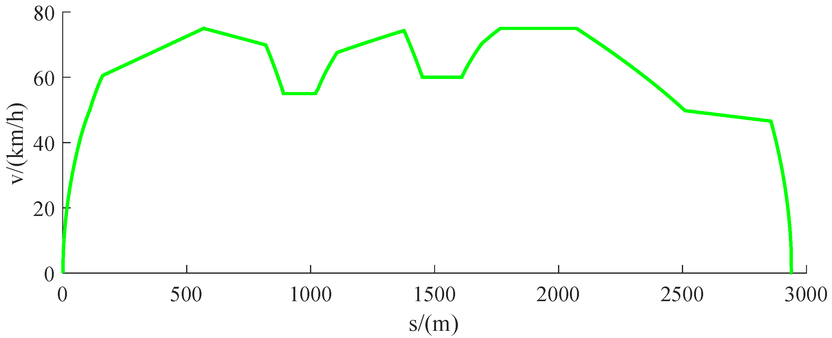
$y_r\left(k\right)$ in Figure 12 is the target speed curve of urban rail train, and its shape is shown in Figure 13.

In Figure 13, the target speed curve can be divided into two cases: the smooth area of curve and the area of curve inflection point. Therefore, we make the following improvements to DMC.

Case 1: The smooth area of curve.

For this area, the target speed curve is smooth. At this point, the softness coefficient $\alpha$ can be appropriately reduced so that the actual output value of the system can quickly track the target speed curve.

Case 2: The area of curve inflection point.

For this area, the speed has sudden change. At this point, the softness coefficient $\alpha$ can be appropriately increased so that the actual output speed of the system can closely track the target speed as much as possible.

4. Results and Discussion

4.1. Relevant Data on Urban Rail Train

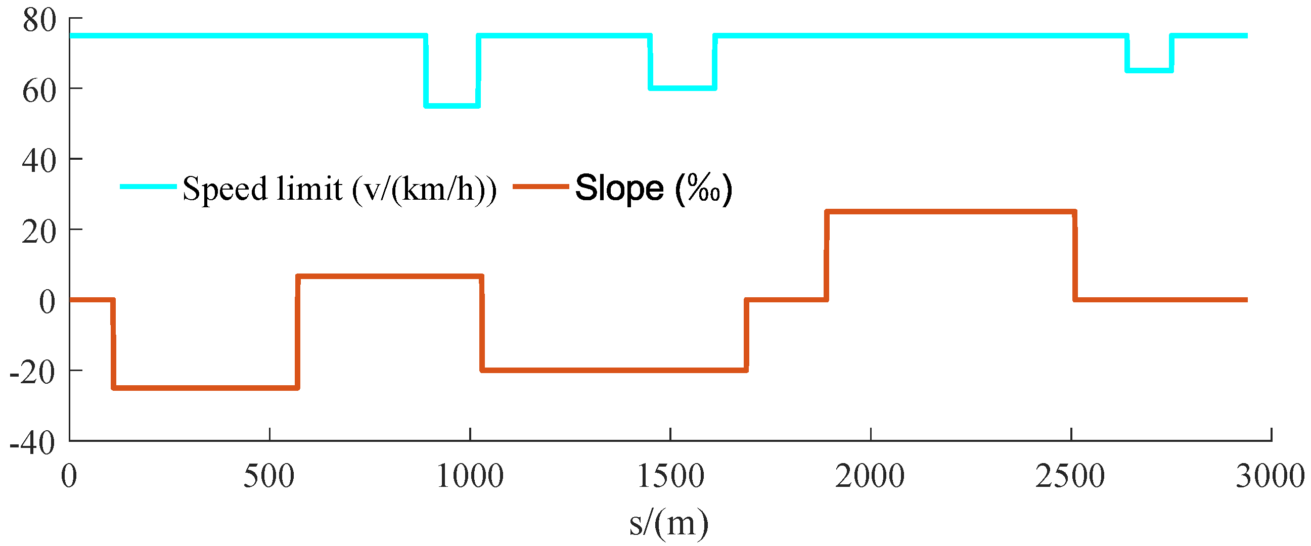
In order to verify the effectiveness of IGA and IDMC for ATO system of urban rail train, the train of light rail line 12 in Dalian, China is selected as the research object. Simulation interval is from New port in Lvshun to Tieshan town, the length of which is 2.94 km. The simulation interval contains three different speed limit subintervals: 50 km/h, 60 km/h, and 65 km/h. The speed limit curve and ramp value curve of this interval are shown in Figure 14, and the properties of the train are shown in

Table 2. The properties of the train.

Parameter Name	Parameter Characteristics
Maximum running speed (km/h)	75
Train weight (t)	105
Rotary mass coefficient $\left(\gamma \right)$	0.06
Electromechanical efficiency of the whole train $\left(\eta \right)$	0.86
Auxiliary power (kW)	300

.

4.2. Optimization of Target Speed Curve for Urban Rail Train

When the urban rail train tracks the target curve, it can guarantee multiple performance indexes of the train, such as safety, energy saving, comfort, stopping accuracy, and punctuality. Therefore, the target speed curve is very important to the operation of the urban rail train. In this paper, the multi-objective optimization model of urban rail train is solved by using basic genetic algorithm (BGA) and IGA. For the multi-objective optimization model, the weight coefficients of $En,Co,Pa$, and $Pu$ are 0.4121, 0.2981, 0.1901, and 0.0997, respectively. For BGA and IGA, the population size is 100; the maximum number of iterations is 200; and the crossover and mutation probabilities are 0.8 and 0.02, respectively. For the simulation interval, the specified run time of the train is 180 s and the requirements of the optimization indexes are $En\in \left[\mathrm{80,000},\mathrm{120,000}\right],Co\in \left[13,30\right],Pa\in [0,0.3]$, and $Pu\in \left[0,2\right]$. In MATLAB environment, the target speed curves obtained by BGA and IGA are shown in Figure 15, and the results of the optimization indexes are shown in

Table 3. The results of the optimization indexes.

Algorithm	Energy	Comfort	Stopping Accuracy	Punctuality	Weighted-Sum Value
BGA	106,031 KJ	20.2654 m/s${}^2$	0.2956 m	0.1064 s	0.3965
IGA	98,013 KJ	16.6421 m/s${}^2$	0.1121 m	0.0135 s	0.2731

.

In Figure 15, compared with BGA, the target speed curve obtained by IGA is smoother and IGA makes the train maintain the appropriate speed more steadily, which can make passengers feel more comfortable. Moreover, these two curves do not exceed the speed limit, which satisfies the safety performance. In Table 3, the energy consumption obtained by IGA is 7.56% lower than that obtained by BGA; the comfort obtained by IGA is 17.88% better than that obtained by BGA; the stopping accuracy obtained by IGA is 62.08% higher than that obtained by BGA; and the punctuality obtained by IGA is 87.31% higher than that obtained by BGA. Therefore, compared with BGA, IGA improved all four optimization indexes of the train, especially stopping accuracy and punctuality. Therefore, we choose the target speed curve obtained by IGA as the input of the speed controller for ATO system.

4.3. Tracking Control of Target Speed Curve for Urban Rail Train

The control algorithm of ATO makes the train run as close to the target curve as possible, and it has direct impact on the performance indexes of the train. IDMC is used to control the ATO system, and multiple performance indexes of ATO system are analyzed, thus verifying the feasibility of IDMC in the ATO system. In order to better illustrate the tracking control effect of IDMC on the target speed curve, the tracking effect of IDMC’s speed controller is compared with that of PID’s speed controller in MATLAB simulation environment. Finally, by analyzing the simulation results of the safety, energy saving, comfort, accurate stopping, and punctuality of the train, the effectiveness of the designed IDMC in controlling the train’s speed is verified.

4.3.1. Analysis of Train’s Safety

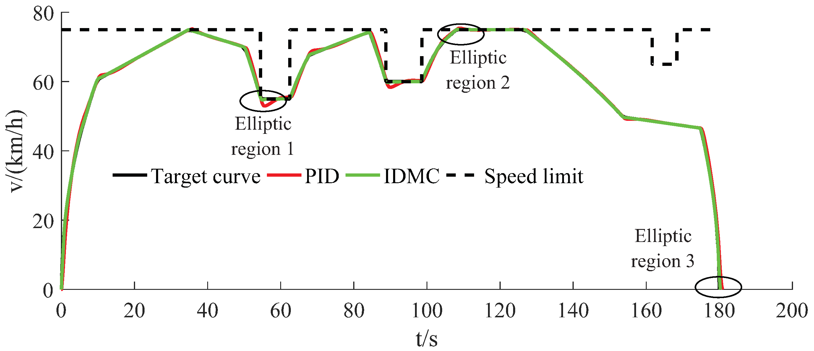
Safety means that the train can run in accordance with the specified line and the actual speed of train cannot exceed the speed limit. Generally speaking, when the actual running speed of the train deviates from the speed limit by less than 7.2 km/h, the train is considered to have good safety performance. The speed time tracking curve is shown in Figure 16.

In Figure 16, under the control of IDMC and PID, the train keeps close to the target speed curve in the whole running process and does not exceed the speed limit. The speed controller of IDMC enables the train’s actual speed to track the target speed curve without large fluctuations, and the actual running curve of the train obtained by IDMC is basically consistent with the target speed curve. For the PID controller, the obvious fluctuation appears in the process of tracking the target curve. Therefore, it verifies that the speed controller of IDMC has better tracking performance than PID controller.

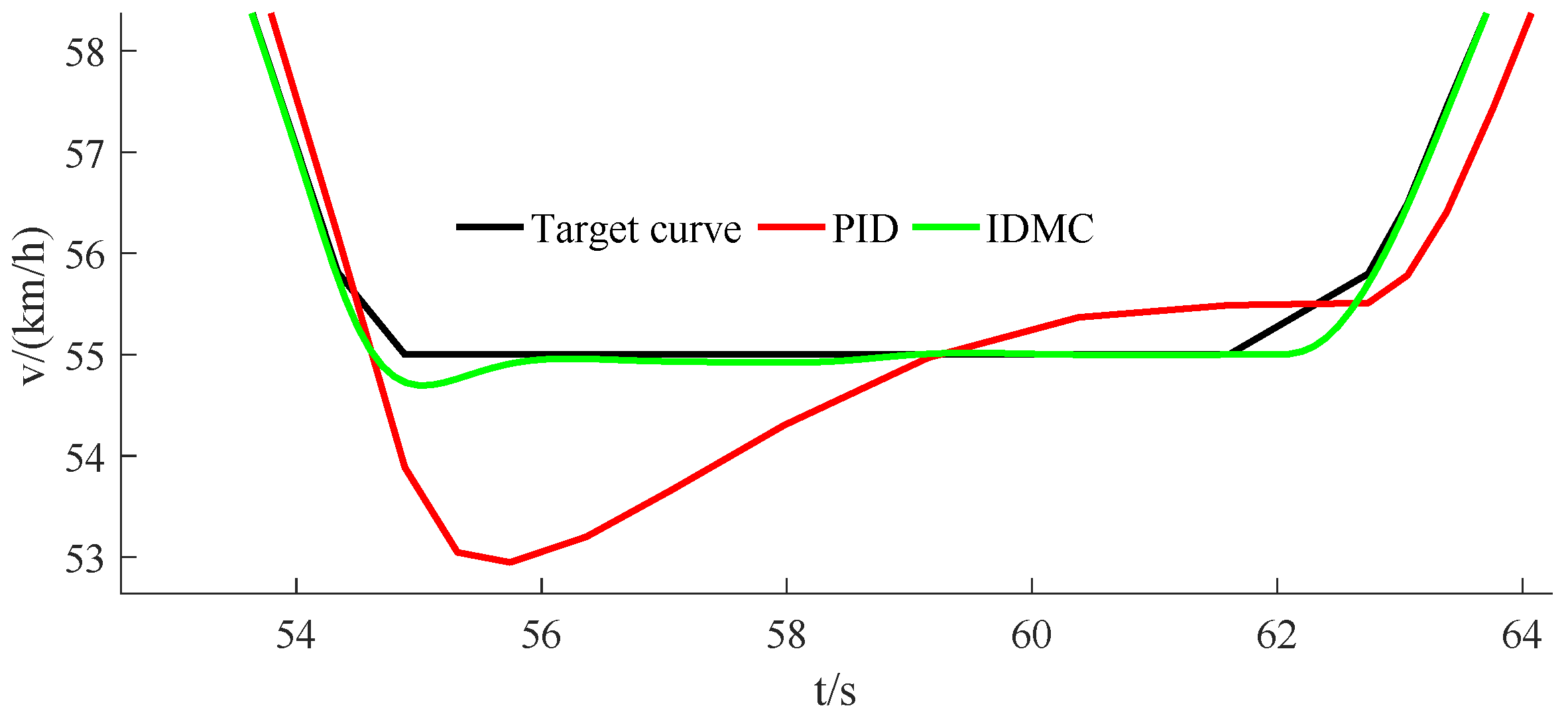
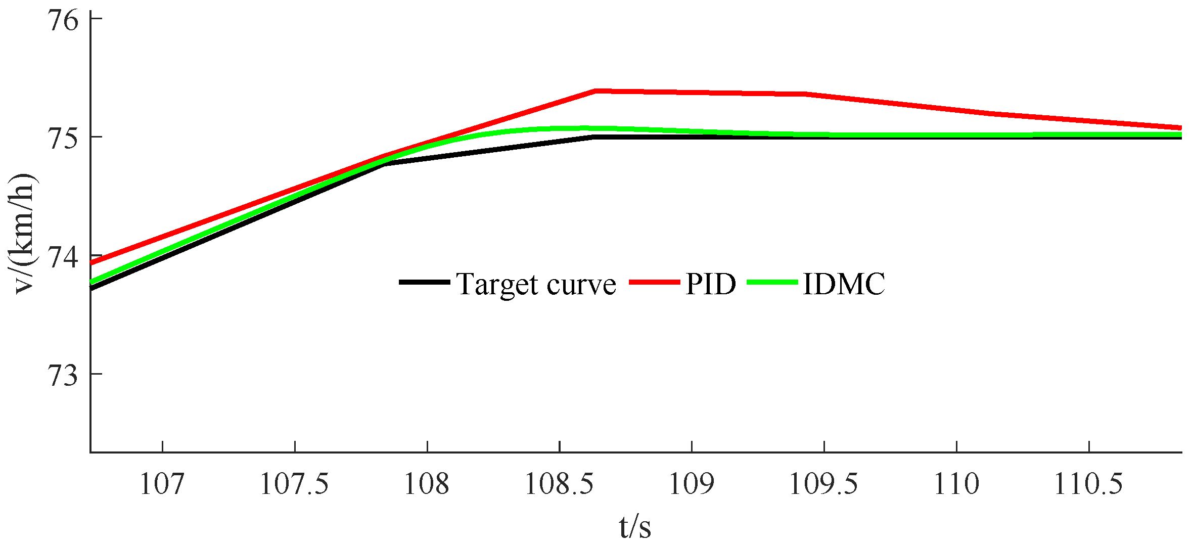
The elliptic region 1 and elliptic region 2 in Figure 16 are locally enlarged, as shown in Figure 17 and Figure 18.

In Figure 17 and Figure 18, for the inflection point area of the target speed curve, the speed curve obtained by IDMC is closer to the target speed curve. However, the speed curve obtained by PID has the big fluctuation. Therefore, the control effect of IDMC is significantly better than PID for the inflection point area of the target speed curve, which indicates that the control accuracy of IDMC on train’s speed is higher than that of PID control.

In conclusion, in the process of train operation, IDMC has higher control accuracy than PID, which can better guarantee the safety of the train.

4.3.2. Analysis of Train’s Energy Consumption

Energy consumption is the energy consumed by the train during the traction and braking stages. According to Equation (7), when the ATO system is controlled by IDMC, the energy consumption of the train is 102,421 KJ. When the ATO system is controlled by PID, the energy consumption of the train is 119,534 KJ. The energy consumption of the train obtained by IDMC is 14.32% lower than that obtained by PID.

4.3.3. Analysis of Train’s Comfort

Comfort is also an important performance index to measure the train operation, which is mainly evaluated by the change of acceleration. When the speed of the train fluctuates greatly, passengers feel obvious discomfort. According to the Equation (9), when the ATO system is controlled by IDMC, the comfort of the train is 41.564 m/s${}^2$. When the ATO system is controlled by PID, the comfort of the train is 68.251 m/s${}^2$. The comfort of the train obtained by IDMC is 39.10% better than that obtained by PID.

4.3.4. Analysis of Train’s Stopping Accuracy

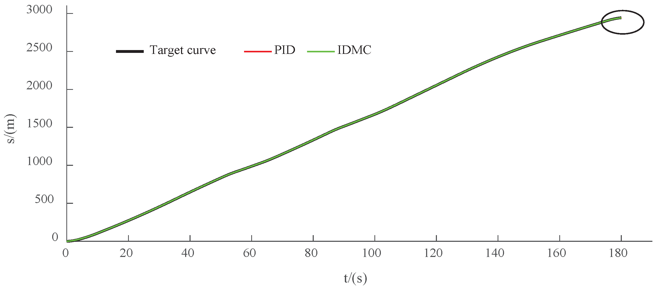
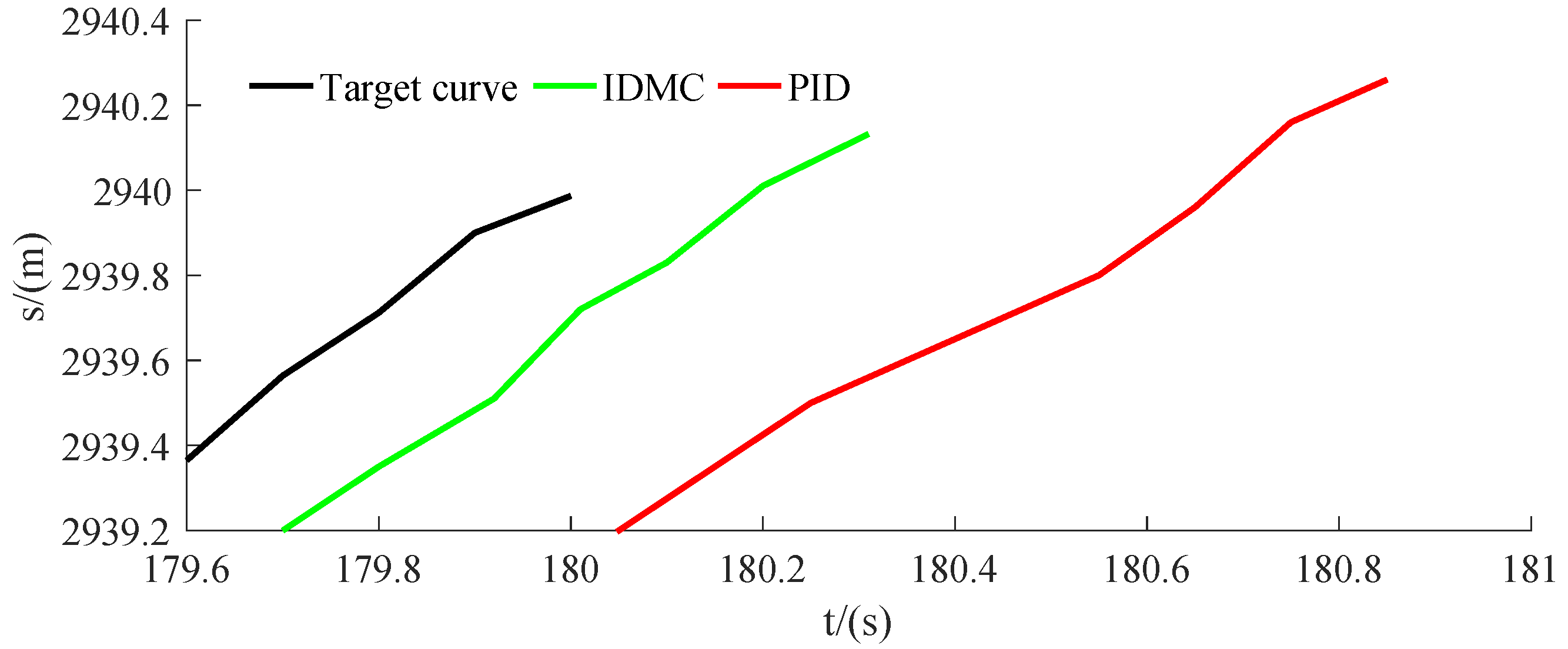
The distance time curve of the train is shown in Figure 19. The elliptic region in Figure 19 is locally enlarged, as shown in Figure 20.

It is ideal that the train can stop at a designated stopping position. However, in the actual operation of the train, there is always the stopping error. Normally, the stopping error of urban rail train should be controlled within 30 cm. The simulation interval from New port in Lvshun to Tieshan town is 2940 m. In Figure 20, when the train is controlled by IDMC, the stopping position of the train is 2940.14 m and the stopping error is 0.14 m. When the train is controlled by PID, the stopping position of the train is 2940.26 m, and the stopping error is 0.26 m. Under the control of IDMC and PID, the stopping errors of the train are within the required range but the control precision of IDMC is higher than that of PID.

4.3.5. Analysis of Train’s Punctuality

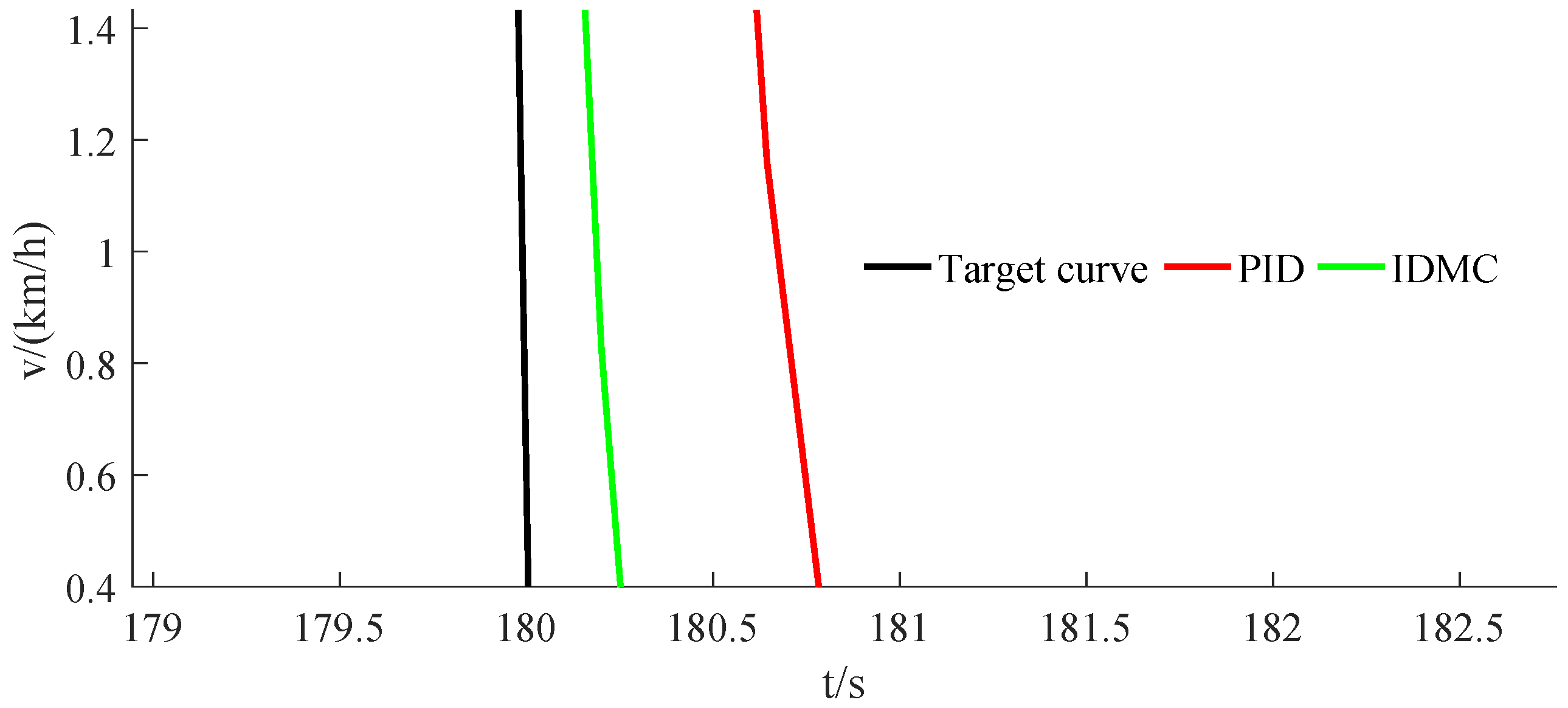
The specified time of simulation interval from New port in Lvshun to Tieshan town is 180 s. The elliptic region 3 in Figure 16 is locally enlarged, as shown in Figure 21.

In Figure 21, when the train is controlled by IDMC, the actual running time of the train is 180.3120 s and the running time error is 0.3120 s. When the train is controlled by PID, the actual running time of the train is 180.8560 s, and the running time error is 0.8560 s. It is obvious that the running time error value of the train obtained by IDMC is less than that obtained by PID. Therefore, the control accuracy of IDMC for the train’s punctuality is higher than PID.

In conclusion, compared with PID, IDMC has the better tracking effect, which can meet the requirements of multiple performance indexes of the train, such as the safety, energy saving, comfort, accurate stopping, and punctuality. In addition, IDMC improves the adaptability and robustness of the speed controller, thus achieving better control effect.

5. Conclusions

This paper introduces the operation principle of ATO system. The ATO system of urban rail train has a two-layer control structure: the upper-layer control and the lower-layer control.

For the upper-layer control, the multi-objective optimization model of urban rail train is built with energy consumption, comfort, stopping accuracy, and punctuality as optimization indexes, and the weight coefficient of each index is solved by entropy weight method. In addition, the force condition of urban rail train is analyzed in detail. Taking the interval from New port in Lvshun to Tieshan town in Dalian, China as an example, the multi-objective model of urban rail train is optimized by using IGA based on directional mutation and gene modification to obtain the target speed curve of the train. The stopping and speed constraints are added into the fitness function of IGA in the form of a penalty function. The results show that the target speed curve obtained by IGA has better performance indexes than BGA.

For the lower-layer control, DMC (a type of predictive control algorithm) is used to design the speed controller of ATO to make the actual speed of the train track the speed of the target curve. DMC directly takes the discrete coefficient of the step response of the object as the model, thus avoiding parameter identification for the transfer function model or the state space equation model. In addition, DMC uses multistep estimation technology, so it can effectively solve the problem of the delay process. However, the inflection point area of the target speed curve is difficult to track, so we improve the basic DMC. The softness factor in the predictive model of DMC should be adjusted online to improve the control accuracy of the speed. The results show that, compared with PID, the improved dynamic matrix control (IDMC) can track target speed curve more accurately and the multiple performance indexes (safety, energy saving, comfort, stopping accuracy, and punctuality) obtained by IDMC are also improved.

Although the speed controller of IDMC is adopted to achieve good tracking effect, it is undeniable that other control algorithms may achieve better control effect for the ATO system. As there are many types of predictive control algorithms, the predictive control algorithms need to be further studied and improved in the future to obtain better results.

References

1. Wang, Y.; Liao, Z.; Tao, T. Train scheduling and circulation planning in urban rail transit lines. Control Eng. Pract. 2017, 61, 112–123. [Google Scholar] [CrossRef]
2. Yang, X.; Li, X.; Ning, B. A Survey on Energy-Efficient Train Operation for Urban Rail Transit. IEEE Trans. Intell. Transp. Syst. 2015, 17, 2–13. [Google Scholar] [CrossRef]
3. Nilsson, J.; Falcone, P.; Vinter, J. Safe Transitions From Automated to Manual Driving Using Driver Controllability Estimation. IEEE Trans. Intell. Transp. Syst. 2015, 16, 1806–1816. [Google Scholar] [CrossRef]
4. Wu, P.; Wang, Q.Y.; Feng, X.Y. Automatic train operation based on adaptive terminal sliding mode control. Int. J. Autom. Comput. 2015, 12, 142–148. [Google Scholar] [CrossRef] [Green Version]
5. Watanabe, S.; Koseki, T.; Isobe, E. Evaluation of Automatic Train Operation Design for Energy Saving Based on the Measured Efficiency of a Linear-Motor Train. Electr. Eng. Jpn. 2018, 202, 460–468. [Google Scholar] [CrossRef]
6. Meng, J.; Xu, R.; Li, D. Combining the Matter-Element Model With the Associated Function of Performance Indices for Automatic Train Operation Algorithm. IEEE Trans. Intell. Transp. Syst. 2019, 20, 253–263. [Google Scholar] [CrossRef]
7. Yin, J.; Chen, D.; Li, L. Combining the Matter-Element Model With the Associated Function of Performance Indices for Automatic Train Operation Algorithm. IEEE Trans. Intell. Transp. Syst. 2014, 15, 2561–2571. [Google Scholar] [CrossRef]
8. Rong, H.; Yu, C.Z. Multiple Objective of Train Operation Process Based on Modified Particle Swarm Optimization. Appl. Mech. Mater. 2014, 513–517, 2927–2930. [Google Scholar] [CrossRef]
9. Liang, Y.; Liu, H.; Qian, C. A Modified Genetic Algorithm for Multi-Objective Optimization on Running Curve of Automatic Train Operation System Using Penalty Function Method. Int. J. Intell. Transp. Syst. Res. 2019, 17, 74–87. [Google Scholar] [CrossRef]
10. Zhao, N.; Roberts, C.; Hillmansen, S. A Multiple Train Trajectory Optimization to Minimize Energy Consumption and Delay. IEEE Trans. Intell. Transp. Syst. 2015, 16, 1–10. [Google Scholar] [CrossRef]
11. Gu, Q.; Tang, T.; Cao, F. Energy-Efficient Train Operation in Urban Rail Transit Using Real-Time Traffic Information. IEEE Trans. Intell. Transp. Syst. 2014, 15, 1216–1233. [Google Scholar] [CrossRef]
12. Lu, S.; Hillmansen, S.; Ho, T.K. Single-Train Trajectory Optimization. IEEE Trans. Intell. Transp. Syst. 2013, 14, 743–750. [Google Scholar] [CrossRef]
13. Pham, H.A. Truss optimization with frequency constraints using enhanced differential evolution based on adaptive directional mutation and nearest neighbor comparison. Adv. Eng. Softw. 2016, 102, 124–154. [Google Scholar] [CrossRef]
14. Bayram, İ.; Haji, S.A.; Cool, G. A Penalty Function Promoting Individual Sparsity in Groups. IEEE Trans. Signal Process. 2016, 65, 4238–4251. [Google Scholar] [CrossRef]
15. Sadiq, R.; Bulek, S. Using penalty functions to evaluate aggregation models for environmental indices. J. Environ. Manag. 2010, 91, 706–716. [Google Scholar] [CrossRef] [PubMed]
16. Gao, S.; Dong, H.; Ning, B. Adaptive fault-tolerant automatic train operation using RBF neural networks. Neural Comput. Appl. 2015, 26, 141–149. [Google Scholar] [CrossRef]
17. Ganesan, M.; Ezhilarasi, D. Hybrid model reference adaptive second order sliding mode controller for automatic train operation. IET Control Theory Appl. 2017, 11, 1222–1233. [Google Scholar]
18. Li, Z.; Hou, Z. Adaptive Iterative Learning Control Based High Speed Train Operation Tracking Under Iteration-Varying Parameter and Measurement Noise. Asian J. Control 2017, 17, 1779–1788. [Google Scholar] [CrossRef]
19. Cao, Y.; Ma, L.; Zhang, Y. Application of fuzzy predictive control technology in automatic train operation. Clust. Comput. 2018, 1–10. [Google Scholar] [CrossRef]
20. Chang, C.S.; Xu, D.Y.; Quek, H.B. Pareto-optimal set based multiobjective tuning of fuzzy automatic train operation for mass transit system. IEE Proc. Electr. Power Appl. 1999, 146, 577–593. [Google Scholar] [CrossRef]
21. Gao, S.; Dong, H.; Chen, Y. Approximation-Based Robust Adaptive Automatic Train Control: An Approach for Actuator Saturation. IEEE Trans. Intell. Transp. Syst. 2013, 14, 1733–1742. [Google Scholar] [CrossRef]
22. Shen, H.; Yan, J. Optimal control of rail transportation associated automatic train operation based on fuzzy control algorithm and PID algorithm. Autom. Control Comput. Sci. 2017, 51, 435–441. [Google Scholar] [CrossRef]
23. Aufderheide, B.; Bequette, B.W. Extension of dynamic matrix control to multiple models. Comput. Chem. Eng. 2003, 27, 1079–1096. [Google Scholar] [CrossRef]
24. Moon, U.; Lee, K.Y. Step-Response Model Development for Dynamic Matrix Control of a Drum-Type Boiler–Turbine System. IEEE Trans. Energy Convers. 2009, 24, 423–430. [Google Scholar] [CrossRef]
25. Wang, L.; Cheng, Y.; Zou, J. Battery available power prediction of hybrid electric vehicle based on improved Dynamic Matrix Control algorithms. J. Power Sour. 2014, 261, 337–347. [Google Scholar] [CrossRef]
26. Zhang, L.; Zhou, W.D. Sparse ensembles using weighted combination methods based on linear programming. Pattern Recognit. 2011, 44, 97–106. [Google Scholar] [CrossRef]
27. Zoghi, M.; Ehsani, A.H.; Sadat, M. Optimization solar site selection by fuzzy logic model and weighted linear combination method in arid and semi-arid region: A case study Isfahan-IRAN. Renew. Sustain. Energy Rev. 2017, 68, 986–996. [Google Scholar] [CrossRef]
28. He, Y.; Guo, H.; Jin, M. A linguistic entropy weight method and its application in linguistic multi-attribute group decision making. Nonlinear Dyn. 2016, 84, 399–404. [Google Scholar] [CrossRef]
29. Xu, H.; Chao, M.; Lian, J. Urban flooding risk assessment based on an integrated k-means cluster algorithm and improved entropy weight method in the region of Haikou, China. J. Hydrol. 2018, 563, 975–986. [Google Scholar] [CrossRef]
30. Liu, P.; Zhang, X.; Lian, J. Research on the supplier selection of a supply chain based on entropy weight and improved ELECTRE-III method. Int. J. Prod. Res. 2011, 49, 637–646. [Google Scholar] [CrossRef]
31. Höschel, K.; Lakshminarayanan, V. Genetic algorithms for lens design: a review. J. Opt. 2019, 48, 134–144. [Google Scholar] [CrossRef]
32. Munroe, S.; Sandoval, K.; Martens, D.E. Genetic algorithm as an optimization tool for the development of sponge cell culture media. In Vitro Cell. Dev. Biol. Anim. 2019, 55, 149–158. [Google Scholar] [CrossRef] [PubMed] [Green Version]
33. Tavakkolimoghaddam, R.; Safari, J.; Sassani, F. Reliability optimization of series-parallel systems with a choice of redundancy strategies using a genetic algorithm. Reliab. Eng. Syst. Saf. 2017, 93, 550–556. [Google Scholar] [CrossRef]
Figure 1. Control principle of the automatic train operation (ATO) system.
Energies 12 03842 g001
Figure 2. Speed tracking of ATO system.
Energies 12 03842 g002
Figure 3. Force condition of urban rail train.
Energies 12 03842 g003
Figure 4. Traction characteristic curve of urban rail train.
Energies 12 03842 g004
Figure 5. Electric braking force curve of urban rail train.
Energies 12 03842 g005
Figure 6. Force condition of urban rail train on the ramp.
Energies 12 03842 g006
Figure 7. Coding of three speed limit subintervals.
Energies 12 03842 g007
Figure 8. The penalty term P e 1 of speed is not 0.
Energies 12 03842 g008
Figure 9. The penalty term P e 2 of stopping error is not 0.
Energies 12 03842 g009
Figure 10. The flow chart of improved genetic algorithm (IGA).
Energies 12 03842 g010
Figure 11. The flow chart of IGA.
Energies 12 03842 g011
Figure 12. The structure of dynamic matrix control (DMC).
Energies 12 03842 g012
Figure 13. Target speed curve of urban rail train.
Energies 12 03842 g013
Figure 14. The speed limit curve and ramp value curve.
Energies 12 03842 g014
Figure 15. The target speed curves obtained by basic genetic algorithm (BGA) and IGA.
Energies 12 03842 g015
Figure 16. The speed time tracking curve.
Energies 12 03842 g016
Figure 17. The elliptic region 1.
Energies 12 03842 g017
Figure 18. The elliptic region 2.
Energies 12 03842 g018
Figure 19. The distance time curve of the train.
Energies 12 03842 g019
Figure 20. The elliptic region in Figure 19.
Energies 12 03842 g020
Figure 21. The elliptic region 3 in Figure 16.
Energies 12 03842 g021