Optimal Strategy to Exploit the Flexibility of an Electric Vehicle Charging Station

 , ,
, ,  ,
,  , and
, and 
Abstract
1. Introduction
1.1. Motivations and Aims
1.2. Literature Review
1.3. Contributions
- minimise the EVCS operation cost, by varying the charging power depending on the energy prices and the charging duration;
- maximise the flexibility capacity (based on Definition 1, presented in Section 2.3), while minimising the EVCS operation cost.
- a dynamic model of an EV battery charger as a flexible load;
- a specific flexibility definition for EV battery chargers;
- a novel formulation for minimising the EVCS operation cost; and
- a novel optimal strategy that maximises the flexibility capacity of EV battery chargers while minimising the EVCS operation cost that leads to providing spinning reserve services.
1.4. Paper Organisation
2. The Electric Vehicle Charging Station Problem
- (i)
- chargers scheduling, also taking into account the uncertainty of the EV arrival time and initial state of charge of the EV battery; and,
- (ii)
- EV load profile management.
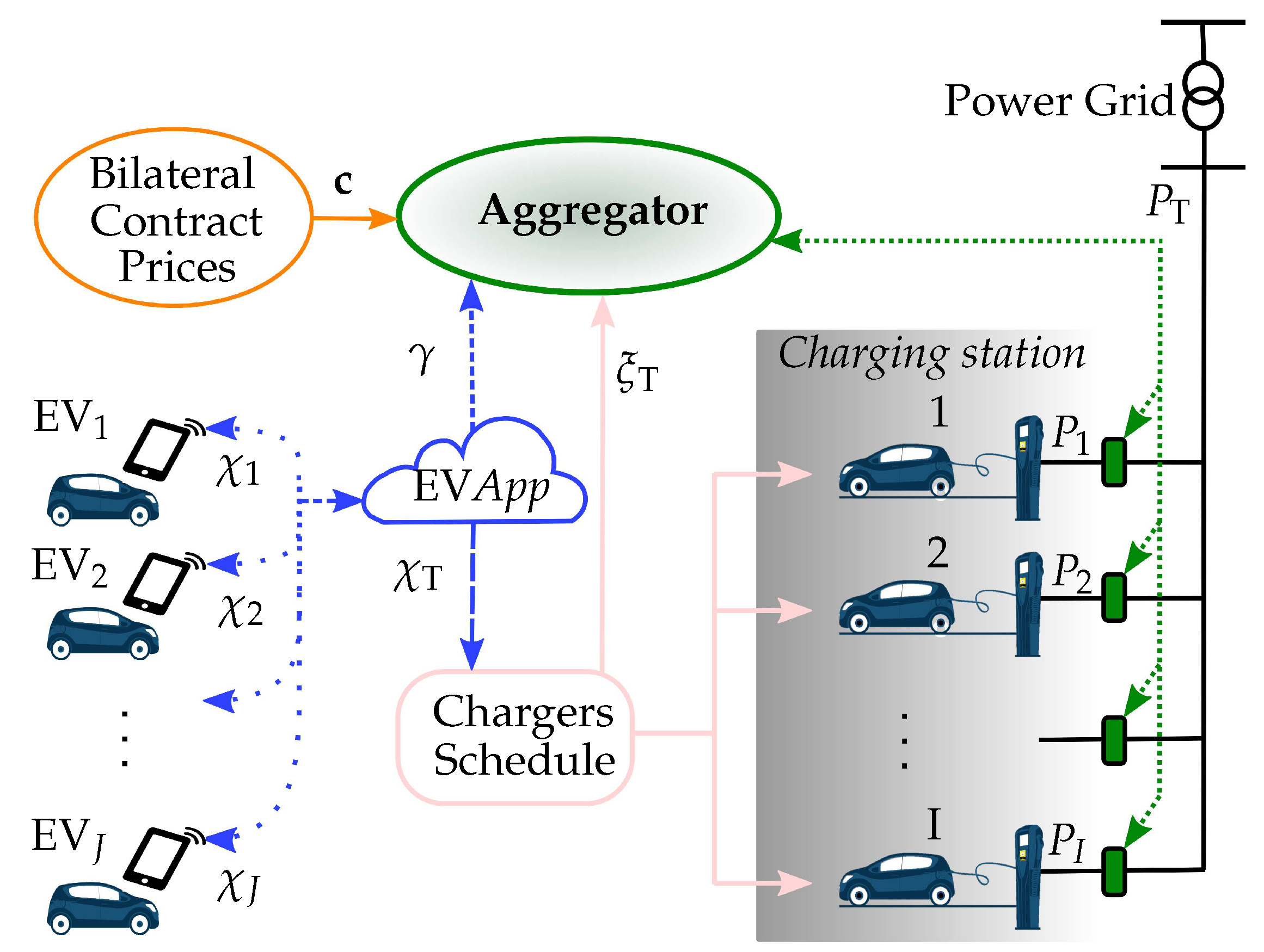
2.1. Charging Station Operations

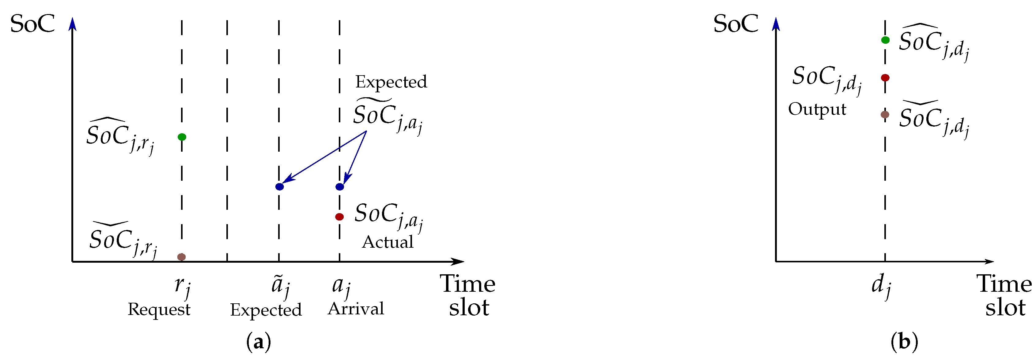
 being the minimum SoC desired by the EV owner at the departure instant , the EV SoC at the request time , and the reported arrival time. Then, the EV owner looks for booking an EV charger from to . Finally, all the EV information to be sent to the charger scheduling algorithm is collected in :, and the actual SoC at the departure . Then, notice that the actual arrival SoC and the reported SoC at the request are generally different, i.e., (see Figure 2a).
- in case of early arrival, nothing changes with respect to the scheduled charging starting instant (); the EV will wait until the scheduled time slot;
- in case of late arrival, up to a given delay , the charging procedure can be performed guaranteeing a departure SoC within the requested limits (see feasible condition Equation (16), presented in Section 3.2);
- in case of late arrival, greater than a given delay , the vehicle is still accepted, but the requested final SoC cannot be guaranteed; and
- the departure time is fixed by the EV owner request, and is considered as a deterministic variable (see Figure 2b).
2.2. The Charger Dynamics Model
2.3. Flexibility Evaluation
constraint and maximum power limits.- Regulation: This service can be provided by units that respond within 15–30 s for fast changes in frequency [63]. In North America, markets like Pennsylvania-New Jersey-Maryland (PJM) [64] and New England [65] call this service Frequency Regulation. Power delivery in this service should last between 10 and 15 min [66].
- Spinning: It is provided by units synchronised to the grid. Units must be fully online within 10 min to provide this service. In addition, this service should be maintained for at least 105 min [67].
- Non-spinning: It is similar to a spinning reserve; the difference is that a non-spinning reserve does not require the permanent synchronisation of the unit to the grid. Units must be totally available within 10 min. Moreover, spinning reserve is more valuable economically for the system operator because it is usually worth 2 to 8 times as much as a non-spinning reserve on an annual average basis [67]. In addition, this service should be maintained for at least 105 min [66].
- Replacement: This service must be supplied within 30 min at the latest, and should be maintained for four hours [68].
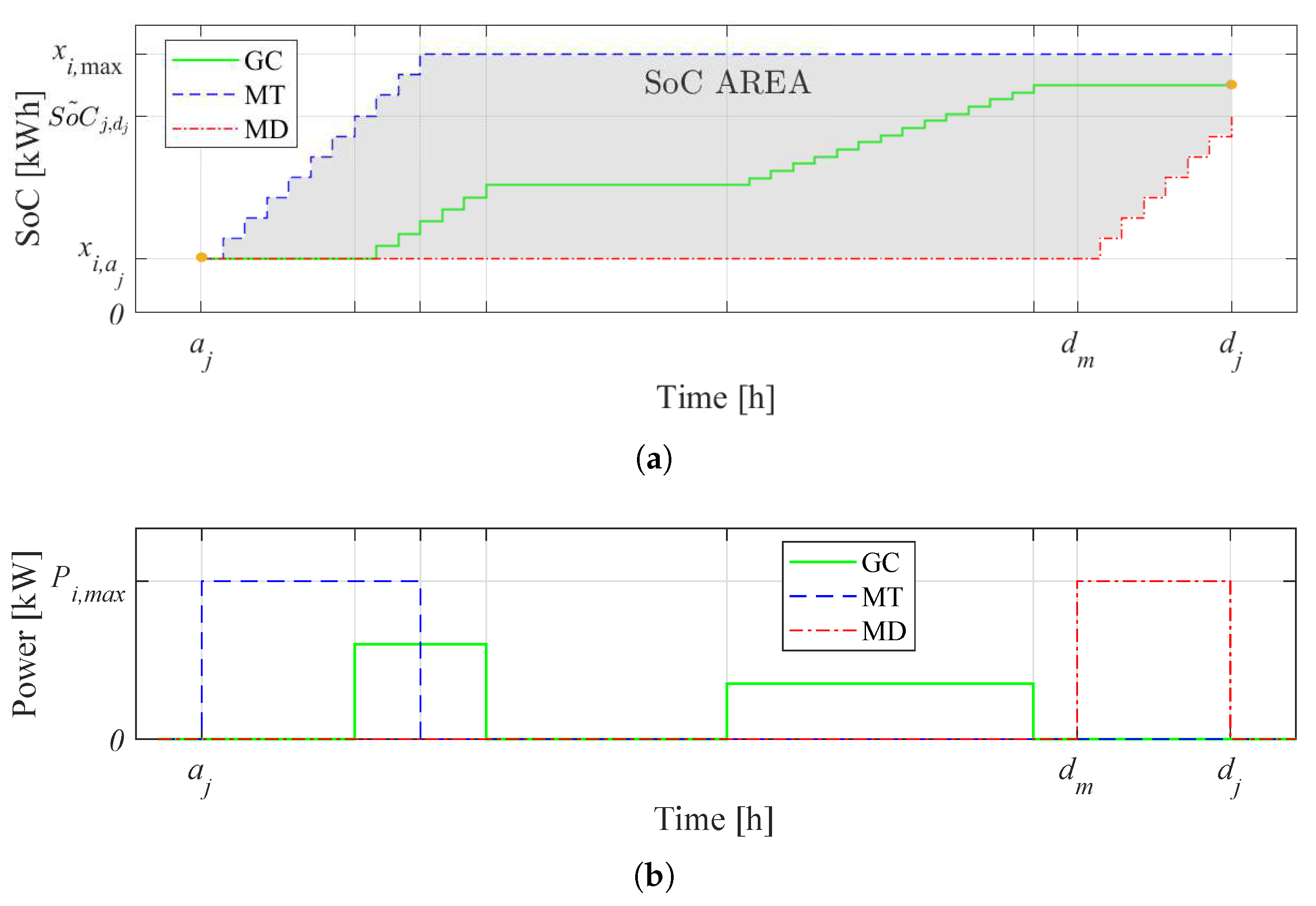
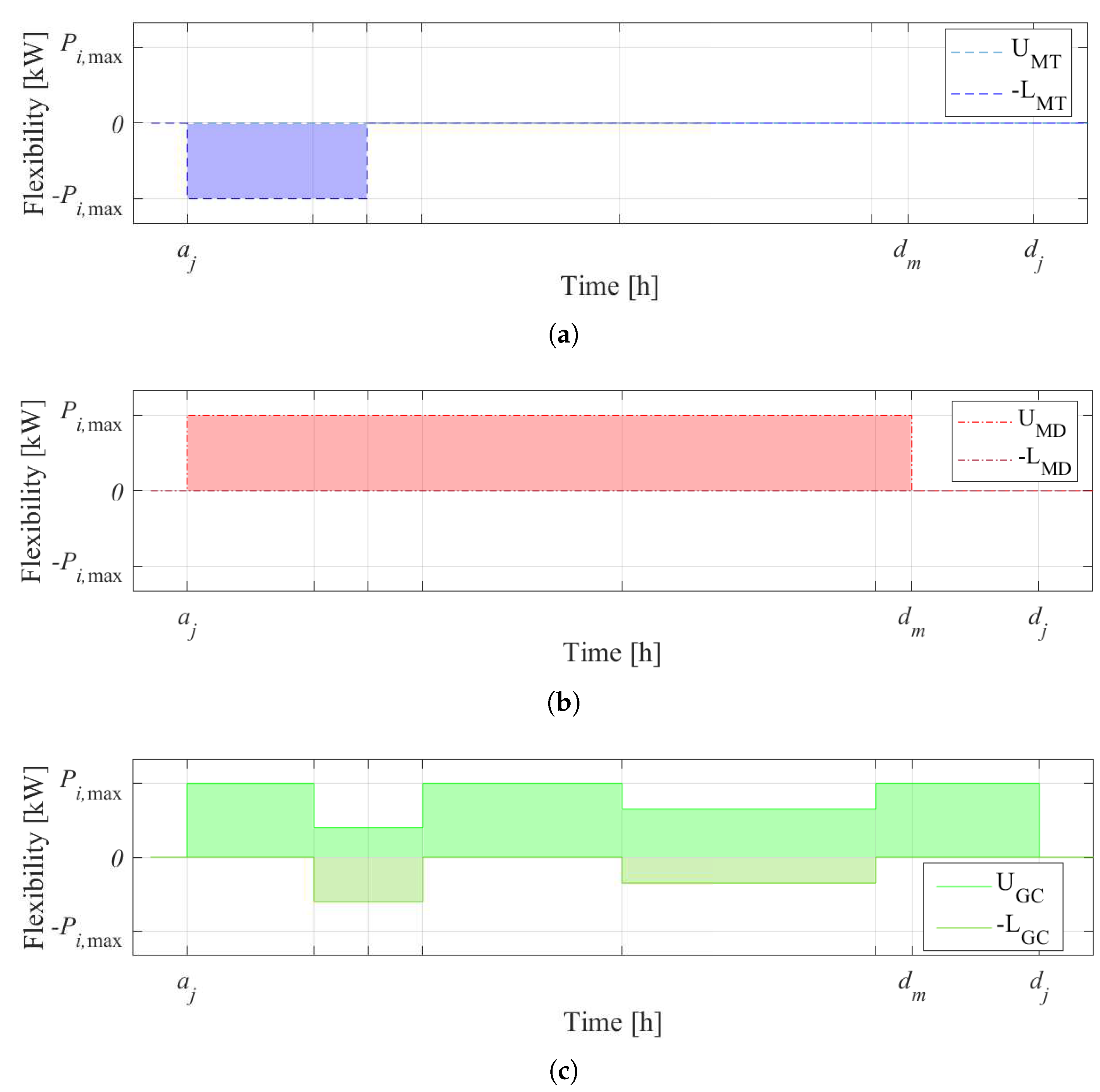
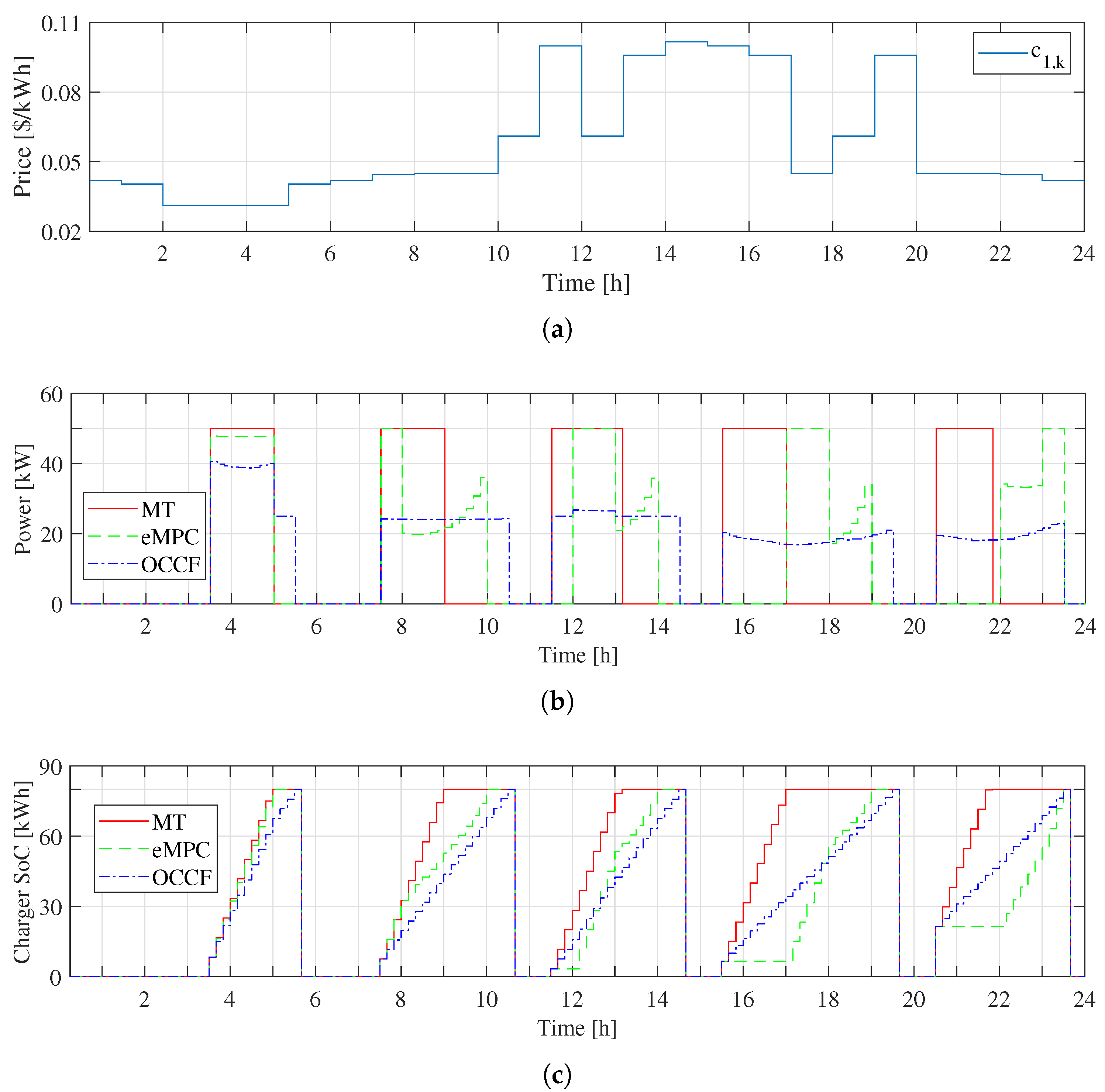
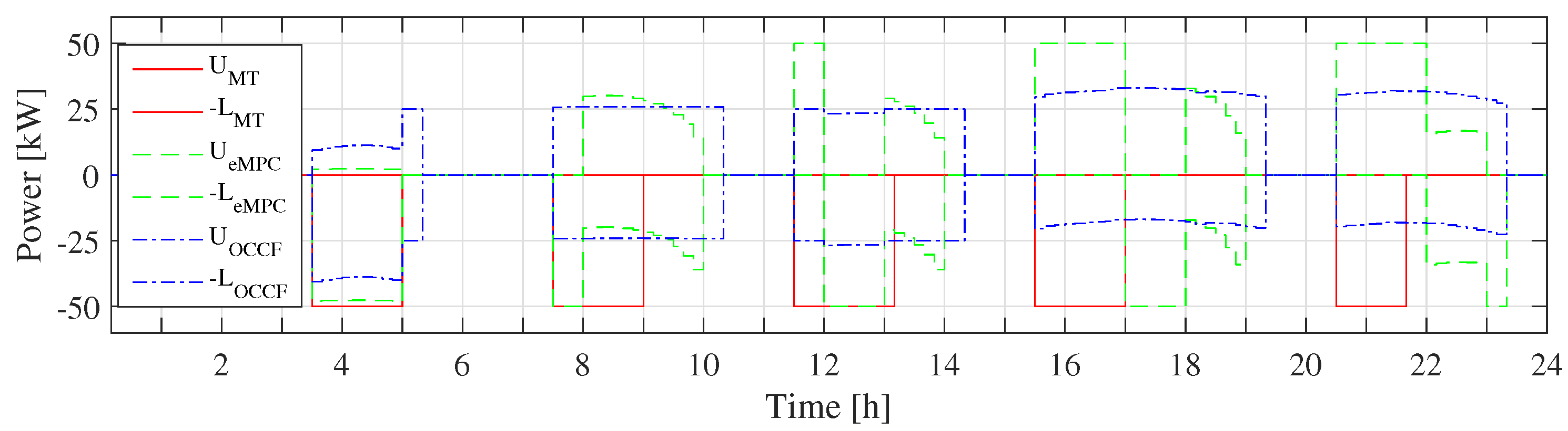
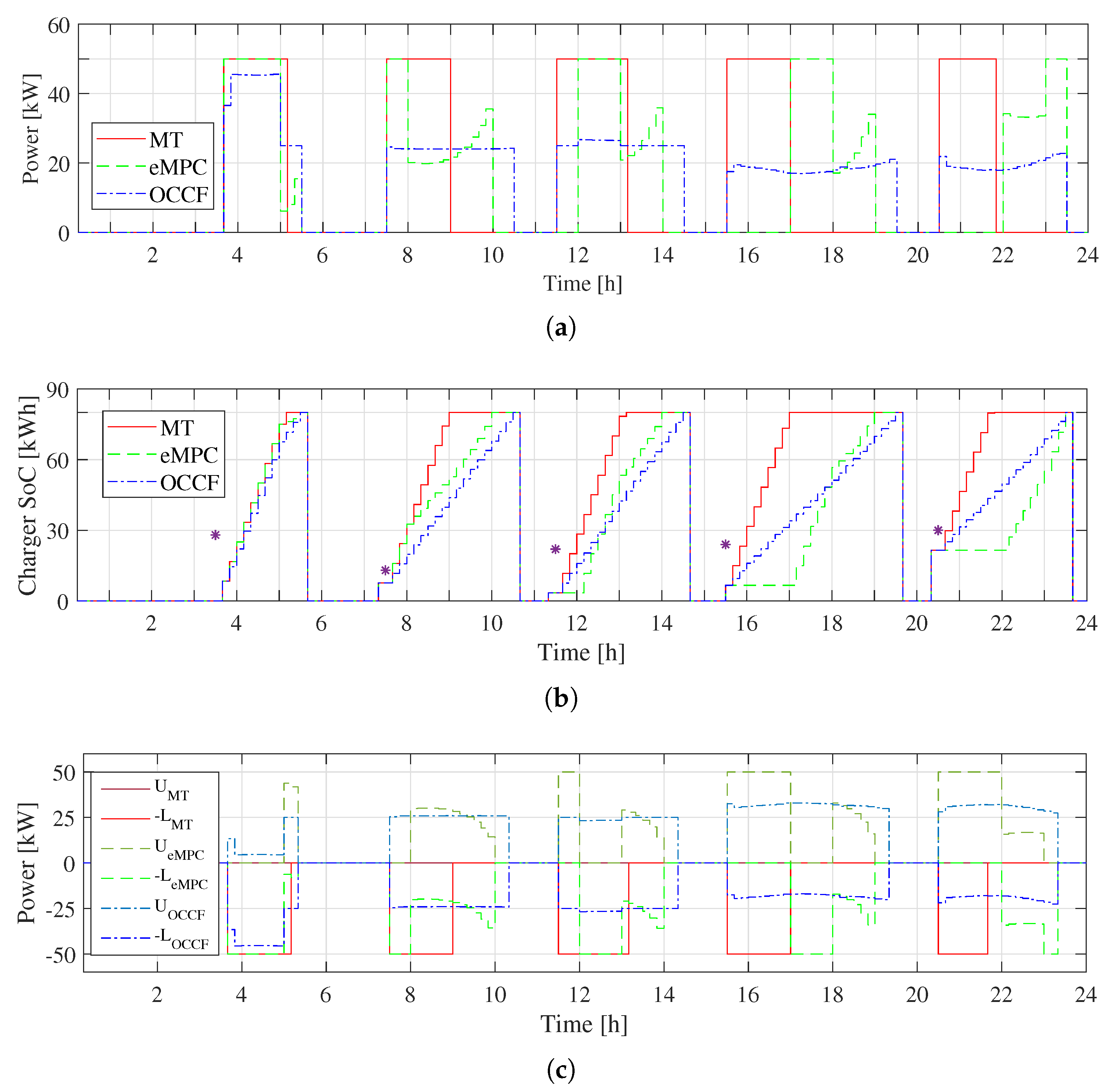
(in this case, no flexibility is possible from to ). Figure 3b depicts the power injected by strategies GC, MT, and MD for creating the SoC area. Note that there are no idle losses due to the short time horizon, and no negative power flows are considered as this work does not take into account V2G applications. , where corresponds to the full charge condition.. Consequently, no charging flexibility is allowed after that instant. In the GC case (Figure 4c), the upward () and the downward () flexibilities are shown. The filled parts indicate the area where the power charging profiles can be adjusted, following profiles of that guarantee not to violate the constraints. It is noteworthy that the SoC might also remain constant for a certain period, e.g., when the EV is not charged, according to the aggregator needs.
3. Solution Strategies
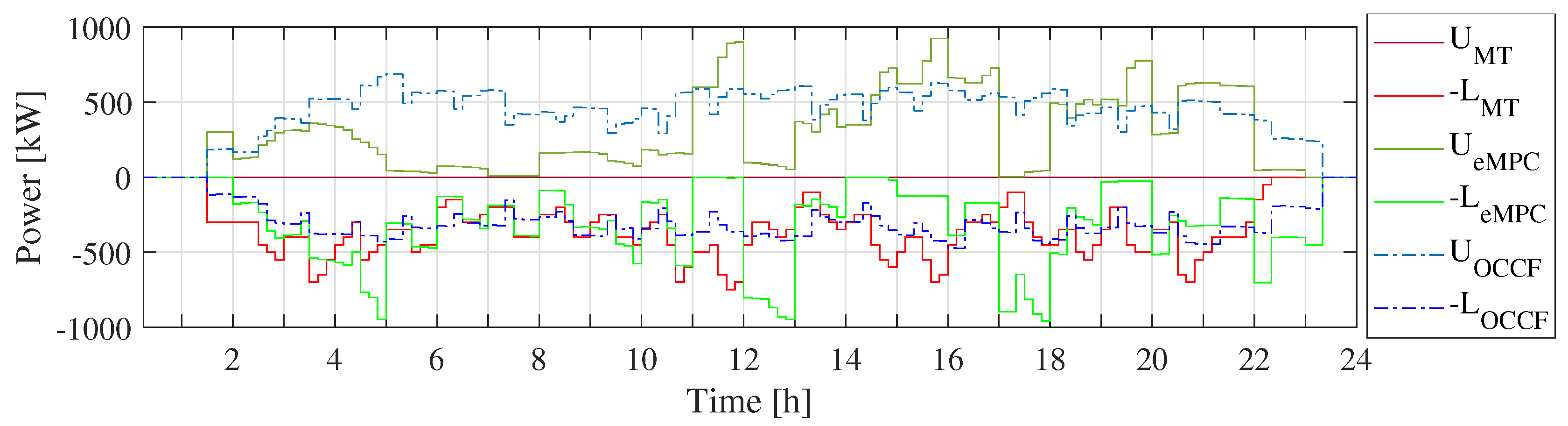
- Minimum Time (MT), as a standard approach, here adopted as a benchmark;
- Optimal Control with minimum Cost and maximum Flexibility (OCCF), a novel strategy based on the Definition 1 presented in Section 2.3.
3.1. Minimum Time as a Benchmark
(full SoC capacity with this strategy) at the departure time, only the EV charging feasibility in a time-span from to is required. This is clarified below.3.2. Economic Model Predictive Control
at the departure time . Thus, by recalling Equation (3), Equation (4) and Equation (7), it holds:
 and the SoC at the request time . Therefore, the actual arrival SoC is lower than the one at the request, i.e., . In addition, the actual arrival time is known within the time interval previous to the connection of the EV to the charger.
 . However, an EV that arrives too late with respect to the request is still allowed to be charged, without guaranteeing that the minimum will be reached.
- the size of the decision and the state variables, and respectively, is ;
- the number of constraints in is , for each time slot, half for the lower bounds, and half for the upper bounds;
- the number of constraints in is , for each time slot; equally allocated among the lower and the upper bounds, and the charger dynamics;
- the number of constraints in , related to the minimum SoC requirement
 at the departure, is I.
3.3. Optimal Control with Minimum Cost and Maximum Flexibility
at the departure time. The uncertainty in the EV arrival time and SoC at the arrival time are considered as in Section 3.2.
4. Case Study and Results
- Minimum time (MT).
- Economic MPC (eMPC).
- MPC with minimum cost and flexibility maximisation (OCCF).
 ), in order to make a meaningful comparison with the MT strategy, in which the EVs are fully charged at the end of the period. Regarding the uncertain parameters, the actual arrival time for each EV is generated as a sample of a random variable with uniform distribution, mean value given by the declared arrival time , and support between , with min. This variability leads to a feasible problem, considering that the minimum interval an EV owner can book a charger is 2 h (see Equation (16)). Then, in the worst case, a charging time of 1 h and 40 min is enough time for charging an EV with the given characteristics, by injecting the maximum feasible power. Moreover, the actual EV arrival state of charge is generated as a sample of a uniform distribution with support between the reported SoC at the request and , where, without loss of generality, is a random number between 15% and 40% of the EV capacity, and
  . In addition, for the MPC algorithm, the expected value is considered as a random value lower than and higher than zero.
4.1. Charger Flexibility Analysis
4.1.1. Deterministic Performance
4.1.2. Results with Uncertainty in Arrival SoC and Arrival Time
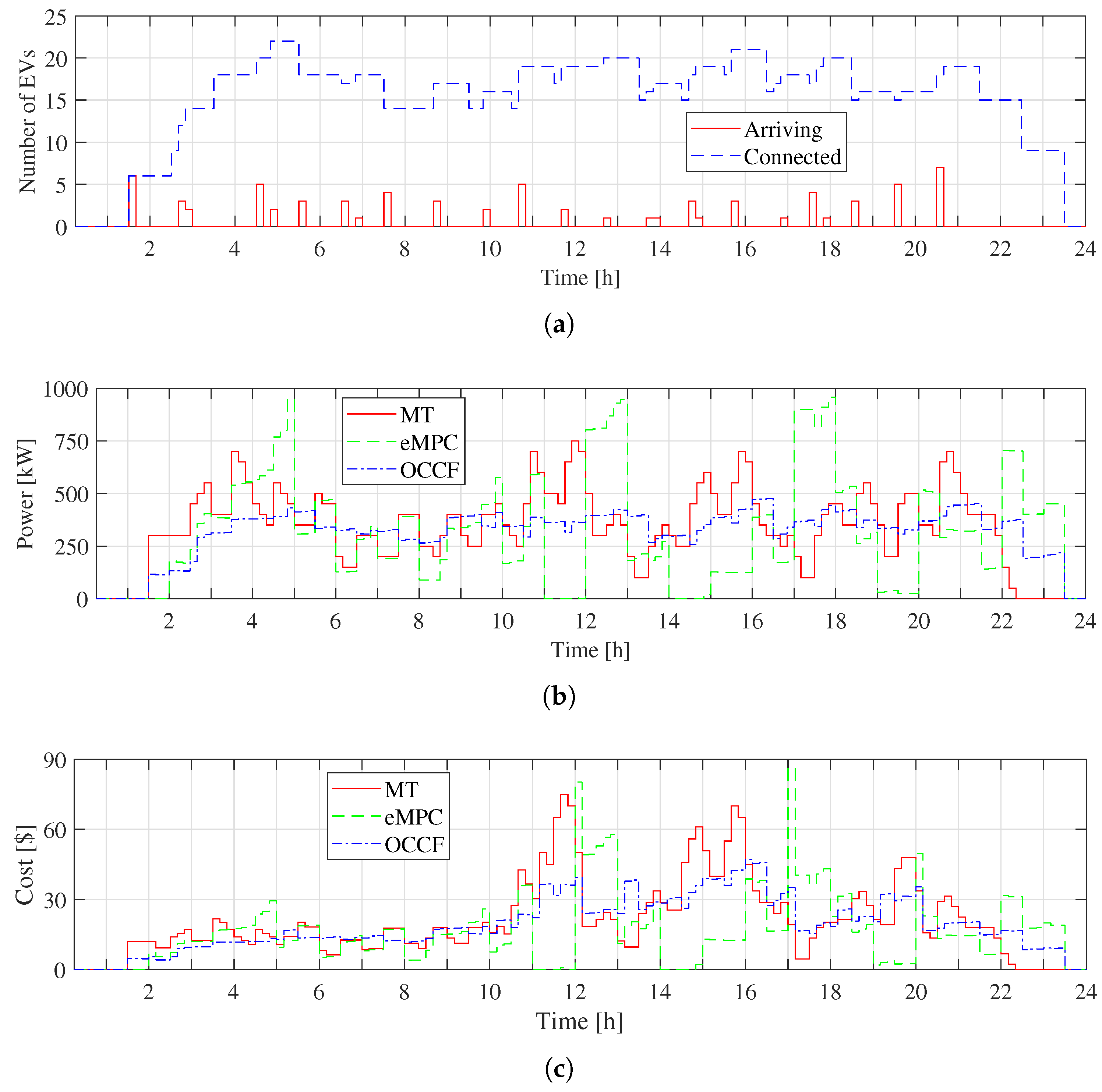
4.2. Savings, Benefits, and Flexibility in the EVCS
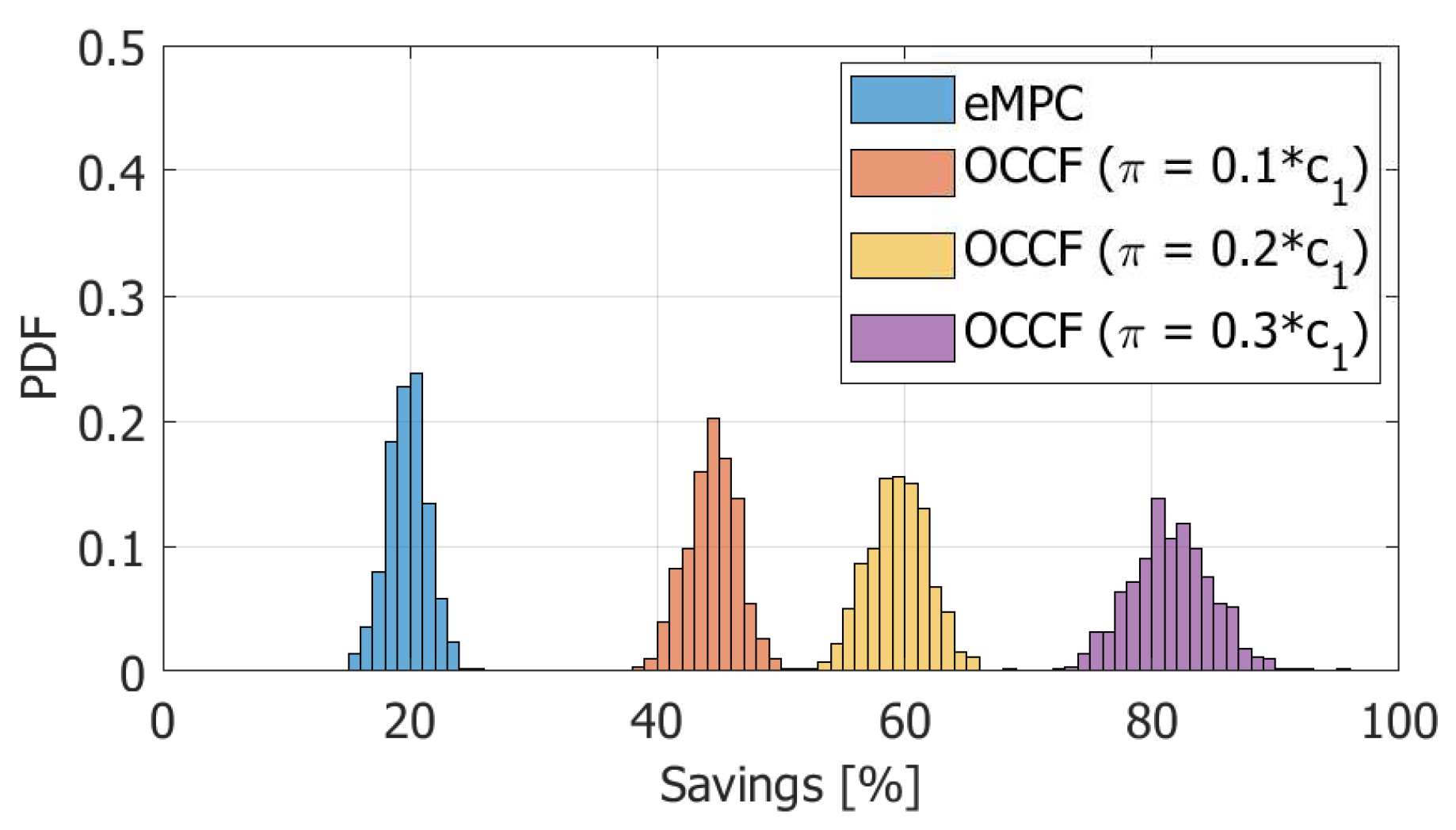
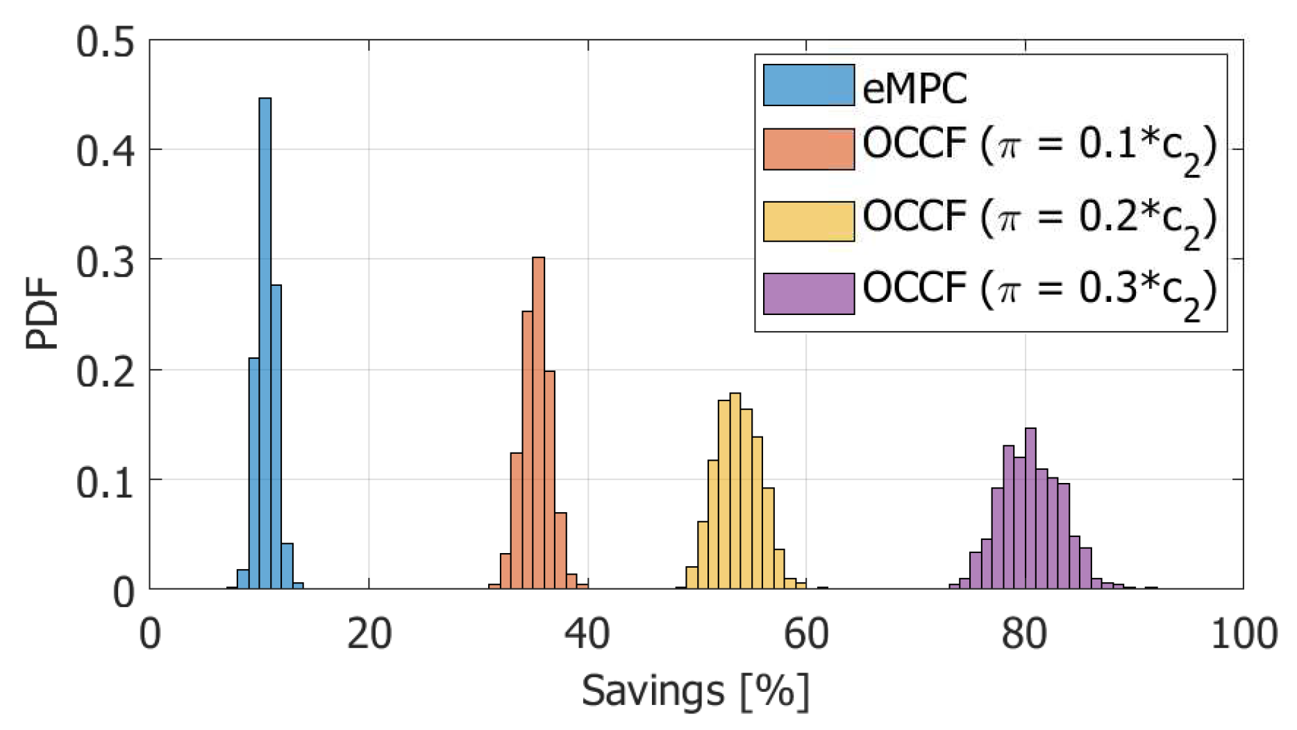
4.3. Monte Carlo Analysis
5. Conclusions
Author Contributions
Funding
Acknowledgments
Conflicts of Interest
References
- U.S. Energy Information Administration. International Energy Outlook 2017. Technical Report; 2017. Available online: www.eia.gov/forecasts/ieo/pdf/0484(2016).pdf (accessed on 11 September 2019).
- Nghitevelekwa, K.; Bansal, R.C. A review of generation dispatch with large-scale photovoltaic systems. Renew. Sustain. Energy Rev. 2018, 81, 615–624. [Google Scholar] [CrossRef]
- Bakirtzis, E.A.; Simoglou, C.K.; Biskas, P.N.; Bakirtzis, A.G. Storage management by rolling stochastic unit commitment for high renewable energy penetration. Electr. Power Syst. Res. 2018, 158, 240–249. [Google Scholar] [CrossRef]
- Pandurangan, V.; Zareipour, H.; Malik, O. Frequency Regulation Services: A Comparative Study of Select North American and European Reserve Markets. In Proceedings of the 2012 North American Power Symposium (NAPS), Champaign, IL, USA, 9–11 September 2012; pp. 1–8. [Google Scholar]
- Deng, R.; Yang, Z.; Chow, M.Y.; Chen, J. A Survey on Demand Response in Smart Grids: Mathematical Models and Approaches. IEEE Trans. Ind. Inform. 2015, 11, 570–582. [Google Scholar] [CrossRef]
- Ma, J.; Silva, V.; Belhomme, R.; Kirschen, D.S.; Ochoa, L.F. Evaluating and Planning Flexibility in Sustainable Power Systems. IEEE Trans. Sustain. Energy 2013, 4, 200–209. [Google Scholar] [CrossRef]
- Holttinen, H.; Tuohy, A.; Milligan, M.; Silva, V.; Müller, S.; Söder, L. The Flexibility Workout: Managing Variable Resources and Assessing the Need for Power System Modification. IEEE Power Energy Mag. 2013, 11, 53–62. [Google Scholar] [CrossRef]
- Ulbig, A.; Andersson, G. Analyzing operational flexibility of electric power systems. Int. J. Electr. Power Energy Syst. 2015, 72, 155–164. [Google Scholar] [CrossRef]
- Li, J.; Liu, F.; Li, Z.; Shao, C.; Liu, X. Grid-side flexibility of power systems in integrating large-scale renewable generations: A critical review on concepts, formulations and solution approaches. Renew. Sustain. Energy Rev. 2018, 93, 272–284. [Google Scholar] [CrossRef]
- Hao, H.; Sanandaji, B.M.; Poolla, K.; Vincent, T.L. Aggregate Flexibility of Thermostatically Controlled Loads. IEEE Trans. Power Syst. 2015, 30, 189–198. [Google Scholar] [CrossRef]
- Zhao, L.; Zhang, W. A Geometric Approach to Aggregate Flexibility Modeling of Thermostatically Controlled Loads. IEEE Trans. Power Syst. 2017, 32, 4721–4731. [Google Scholar] [CrossRef]
- Sajjad, I.A.; Chicco, G.; Napoli, R. Definitions of Demand Flexibility for Aggregate Residential Loads. IEEE Trans. Smart Grid 2016, 7, 2633–2643. [Google Scholar] [CrossRef]
- Diaz, C.; Ruiz, F.; Patino, D. Modeling and control of water booster pressure systems as flexible loads for demand response. Appl. Energy 2017, 204, 106–116. [Google Scholar] [CrossRef]
- Papadaskalopoulos, D.; Strbac, G.; Mancarella, P.; Aunedi, M.; Stanojevic, V. Decentralized Participation of Flexible Demand in Electricity Markets—Part II: Application With Electric Vehicles and Heat Pump Systems. IEEE Trans. Power Syst. 2013, 28, 3667–3674. [Google Scholar] [CrossRef]
- Good, N.; Mancarella, P. Flexibility in multi-energy communities with electrical and thermal storage: A stochastic, robust approach for multi-service demand response. IEEE Trans. Smart Grid 2019, 10, 503–513. [Google Scholar] [CrossRef]
- Wang, Y.; Cheng, J.; Zhang, N.; Kang, C. Automatic and linearized modeling of energy hub and its flexibility analysis. Appl. Energy 2018, 211, 705–714. [Google Scholar] [CrossRef]
- Haas, J.; Cebulla, F.; Cao, K.; Nowak, W.; Palma-behnke, R.; Rahmann, C.; Mancarella, P. Challenges and trends of energy storage expansion planning for fl exibility provision in low-carbon power systems—A review. Renew. Sustain. Energy Rev. 2017, 80, 603–619. [Google Scholar] [CrossRef]
- Pavić, I.; Capuder, T.; Kuzle, I. Value of flexible electric vehicles in providing spinning reserve services. Appl. Energy 2015, 157, 60–74. [Google Scholar] [CrossRef]
- Borba, B.S.M.; Szklo, A.; Schaeffer, R. Plug-in hybrid electric vehicles as a way to maximize the integration of variable renewable energy in power systems: The case of wind generation in northeastern Brazil. Energy 2012, 37, 469–481. [Google Scholar] [CrossRef]
- Khemakhem, S.; Rekik, M.; Krichen, L. A flexible control strategy of plug-in electric vehicles operating in seven modes for smoothing load power curves in smart grid. Energy 2017, 118, 197–208. [Google Scholar] [CrossRef]
- Wenzel, G.; Negrete-pincetic, M.; Olivares, D.E.; Macdonald, J.; Callaway, D.S. Real-Time Charging Strategies for an Electric Vehicle Aggregator to Provide Ancillary Services. IEEE Trans. Smart Grid 2018, 9, 5141–5151. [Google Scholar] [CrossRef]
- Giordano, F.; Ciocia, A.; Di Leo, P.; Spertino, F.; Tenconi, A.; Vaschetto, S. Self-Consumption Improvement for a Nanogrid with Photovoltaic and Vehicle-to-Home Technologies. In Proceedings of the 2018 IEEE International Conference on Environment and Electrical Engineering and 2018 IEEE Industrial and Commercial Power Systems Europe (EEEIC/I&CPS Europe), Palermo, Italy, 12–15 June 2018; pp. 1–6. [Google Scholar]
- Noel, L.; Rubens, G.Z.D.; Sovacool, B.K. Optimizing innovation, carbon and health in transport: Assessing socially optimal electric mobility and vehicle-to-grid pathways in Denmark. Energy 2018, 153, 628–637. [Google Scholar] [CrossRef]
- Cao, Y.; Wang, T.; Kaiwartya, O.; Min, G.; Ahmad, N.; Abdullah, A.H. An EV Charging Management System Concerning Drivers’ Trip Duration and Mobility Uncertainty. IEEE Trans. Syst. Man Cybern. Syst. 2018, 48, 596–607. [Google Scholar] [CrossRef]
- García-Villalobos, J.; Zamora, I.; San Martín, J.I.; Asensio, F.J.; Aperribay, V. Plug-in electric vehicles in electric distribution networks: A review of smart charging approaches. Renew. Sustain. Energy Rev. 2014, 38, 717–731. [Google Scholar] [CrossRef]
- Quirós-Tortós, J.; Ochoa, L.; Butler, T. How Electric Vehicles and the Grid Work Together: Lessons Learned from One of the Largest Electric Vehicle Trials in the World. IEEE Power Energy Mag. 2018, 16, 64–76. [Google Scholar] [CrossRef]
- Haidar, A.M.A.; Muttaqi, K.M.; Haque, M.H. Multistage time-variant electric vehicle load modelling for capturing accurate electric vehicle behaviour and electric vehicle impact on electricity distribution grids. IET Gener. Transm. Distrib. 2015, 9, 2705–2716. [Google Scholar] [CrossRef]
- Sundström, O.; Binding, C. Flexible charging optimization for electric vehicles considering distribution grid constraints. IEEE Trans. Smart Grid 2012, 3, 26–37. [Google Scholar] [CrossRef]
- Hu, J.; Morais, H.; Sousa, T.; Lind, M. Electric vehicle fleet management in smart grids: A review of services, optimization and control aspects. Renew. Sustain. Energy Rev. 2016, 56, 1207–1226. [Google Scholar] [CrossRef]
- Schuller, A.; Flath, C.M.; Gottwalt, S. Quantifying load flexibility of electric vehicles for renewable energy integration. Appl. Energy 2015, 151, 335–344. [Google Scholar] [CrossRef]
- Sadeghianpourhamami, N.; Refa, N.; Strobbe, M.; Develder, C. Quantitive analysis of electric vehicle flexibility: A data-driven approach. Int. J. Electr. Power Energy Syst. 2018, 95, 451–462. [Google Scholar] [CrossRef]
- Mills, G.; Macgill, I. Assessing Electric Vehicle storage, flexibility, and Distributed Energy Resource potential. J. Energy Storage 2018, 17, 357–366. [Google Scholar] [CrossRef]
- Munshi, A.A.; Mohamed, Y. Extracting and Defining Flexibility of Residential Electrical Vehicle Charging Loads. IEEE Trans. Ind. Inform. 2018, 14, 448–461. [Google Scholar] [CrossRef]
- Grahn, P.; Alvehag, K.; Söder, L. PHEV Utilization Model Considering Type-of-Trip and Recharging Flexibility. IEEE Trans. Smart Grid 2014, 5, 139–148. [Google Scholar] [CrossRef]
- Clairand, J.M.; Rodríguez-García, J.; Álvarez-Bel, C. Smart Charging for Electric Vehicle Aggregators Considering Users’ Preferences. IEEE Access 2018, 6, 54624–54635. [Google Scholar] [CrossRef]
- Qi, W.; Xu, Z.; Shen, Z.J.M.; Hu, Z.; Song, Y. Hierarchical coordinated control of plug-in electric vehicles charging in multifamily dwellings. IEEE Trans. Smart Grid 2014, 5, 1465–1474. [Google Scholar] [CrossRef]
- Yang, L.; Zhang, J.; Poor, H.V. Risk-aware day-ahead scheduling and real-time dispatch for electric vehicle charging. IEEE Trans. Smart Grid 2014, 5, 693–702. [Google Scholar] [CrossRef]
- Janjic, A.; Velimirovic, L.; Stankovic, M.; Petrusic, A. Commercial electric vehicle fleet scheduling for secondary frequency control. Electr. Power Syst. Res. 2017, 147, 31–41. [Google Scholar] [CrossRef]
- Wang, R.; Xiao, G.; Wang, P. Hybrid Centralized-Decentralized (HCD) Charging Control of Electric Vehicles. IEEE Trans. Veh. Technol. 2017, 66, 6728–6741. [Google Scholar] [CrossRef]
- Pertl, M.; Carducci, F.; Tabone, M.; Marinelli, M.; Kiliccote, S.; Kara, E.C. An Equivalent Time-Variant Storage Model to Harness EV Flexibility: Forecast and Aggregation. IEEE Trans. Ind. Inform. 2019, 15, 1899–1910. [Google Scholar] [CrossRef]
- Esmaili, M.; Goldoust, A. Multi-objective optimal charging of plug-in electric vehicles in unbalanced distribution networks. Int. J. Electr. Power Energy Syst. 2015, 73, 644–652. [Google Scholar] [CrossRef]
- Škugor, B.; Deur, J. Dynamic programming-based optimisation of charging an electric vehicle fleet system represented by an aggregate battery model. Energy 2015, 92, 456–465. [Google Scholar] [CrossRef]
- Sun, B.; Tan, X.; Tsang, D.H.K. Eliciting Multi-dimensional Flexibilities from Electric Vehicles: A Mechanism Design Approach. IEEE Trans. Power Syst. 2018. [Google Scholar] [CrossRef]
- Zhou, B.; Yao, F.; Littler, T.; Zhang, H. An electric vehicle dispatch module for demand-side energy participation. Appl. Energy 2016, 177, 464–474. [Google Scholar] [CrossRef]
- del Razo, V.; Goebel, C.; Jacobsen, H.A. Vehicle-Originating-Signals for Real-Time Charging Control of Electric Vehicle Fleets. IEEE Trans. Transp. Electrif. 2015, 1, 150–167. [Google Scholar] [CrossRef]
- Su, W.; Wang, J.; Zhang, K.; Huang, A.Q. Model predictive control-based power dispatch for distribution system considering plug-in electric vehicle uncertainty. Electr. Power Syst. Res. 2014, 106, 29–35. [Google Scholar] [CrossRef]
- Ruelens, F.; Vandael, S.; Leterme, W.; Claessens, B.J.; Hommelberg, M.; Holvoet, T.; Belmans, R. Demand side management of electric vehicles with uncertainty on arrival and departure times. In Proceedings of the IEEE PES Innovative Smart Grid Technologies Conference Europe, Berlin, Germany, 14–17 October 2012; pp. 1–8. [Google Scholar] [CrossRef]
- Ji, Z.; Huang, X.; Xu, C.; Sun, H. Accelerated model predictive control for electric vehicle integrated microgrid energy management: A hybrid robust and stochastic approach. Energies 2016, 9, 973. [Google Scholar] [CrossRef]
- Halvgaard, R.; Poulsen, N.K.; Madsen, H.; Jørgensen, J.B.; Marra, F.; Bondy, D.E.M. Electric vehicle charge planning using economic model predictive control. In Proceedings of the 2012 IEEE International Electric Vehicle Conference (IEVC 2012), Greenville, SC, USA, 4–8 March 2012; pp. 1–6. [Google Scholar] [CrossRef]
- Diaz, C.; Ruiz, F.; Patino, D. Smart Charge of an Electric Vehicles Station: A Model Predictive Control Approach. In Proceedings of the 2018 IEEE Conference on Control Technology and Applications (CCTA), Copenhagen, Denmark, 21–24 August 2018; pp. 54–59. [Google Scholar] [CrossRef]
- Diaz, C.; Mazza, A.; Ruiz, F.; Patino, D.; Chicco, G. Understanding Model Predictive Control for Electric Vehicle Charging Dispatch. In Proceedings of the 2018 53nd International Universities Power Engineering Conference (UPEC), Glasgow, UK, 4–7 September 2018; pp. 1–6. [Google Scholar]
- Braun, M.W.; Rivera, D.E.; Carlyle, W.M.; Kempf, K.G. A model predictive control framework for robust management of multi-product, multi-echelon demand networks. IFAC Proc. Vol. (IFAC-PapersOnline) 2003, 27, 229–245. [Google Scholar] [CrossRef]
- Oldewurtel, F.; Parisio, A.; Jones, C.N.; Gyalistras, D.; Gwerder, M.; Stauch, V.; Lehmann, B.; Morari, M. Use of model predictive control and weather forecasts for energy efficient building climate control. Energy Build. 2012, 45, 15–27. [Google Scholar] [CrossRef]
- Colmenar-Santos, A.; Muñoz-Gómez, A.M.; Rosales-Asensio, E.; López-Rey, Á. Electric vehicle charging strategy to support renewable energy sources in Europe 2050 low-carbon scenario. Energy 2019, 183, 61–74. [Google Scholar] [CrossRef]
- Naharudinsyah, I.; Limmer, S. Optimal Charging of Electric Vehicles with Trading on the Intraday Electricity Market. Energies 2018, 11, 1416. [Google Scholar] [CrossRef]
- Mouli, G.R.C.; Kaptein, J.; Bauer, P.; Zeman, M. Implementation of dynamic charging and V2G using Chademo and CCS/Combo DC charging standard. In Proceedings of the 2016 IEEE Transportation Electrification Conference and Expo (ITEC 2016), Dearborn, MI, USA, 27–29 June 2016; pp. 1–6. [Google Scholar] [CrossRef]
- Open Charge Alliance. Open Charge Point Protocol 1.6. Technical Report. 2015. Available online: https://www.openchargealliance.org/ (accessed on 11 September 2019).
- Amjad, M.; Ahmad, A.; Rehmani, M.H.; Umer, T. A review of EVs charging: From the perspective of energy optimization, optimization approaches, and charging techniques. Transp. Res. Part Transp. Environ. 2018, 62, 386–417. [Google Scholar] [CrossRef]
- Hoke, A.; Brissette, A.; Smith, K.; Pratt, A. Accounting for Lithium-Ion Battery Degradation in Electric Vehicle Charging Optimization. IEEE J. Emerg. Sel. Top. Power Electron. 2014, 2, 691–700. [Google Scholar] [CrossRef]
- Ottesen, S.Ø.; Tomasgard, A.; Fleten, S.E. Multi market bidding strategies for demand side flexibility aggregators in electricity markets. Energy 2018, 149, 120–134. [Google Scholar] [CrossRef]
- Lund, P.D.; Lindgren, J.; Mikkola, J.; Salpakari, J. Review of energy system flexibility measures to enable high levels of variable renewable electricity. Renew. Sustain. Energy Rev. 2015, 45, 785–807. [Google Scholar] [CrossRef]
- González, P.; Villar, J.; Díaz, C.A.; Campos, F.A. Joint energy and reserve markets: Current implementations and modeling trends. Electr. Power Syst. Res. 2014, 109, 101–111. [Google Scholar] [CrossRef]
- Baccino, F.; Conte, F.; Massucco, S.; Silvestro, F.; Grillo, S. Frequency Regulation by Management of Building Cooling Systems through Model Predictive Control. In Proceedings of the 18th Power Systems Computation Conference (PSCC), Wroclaw, Poland, 18–22 August 2014; pp. 1–7. [Google Scholar] [CrossRef]
- PJM Forward Market Operations. PJM Manual 11: Energy and Ancillary Services Market Operations; PJM: Audubon, PA, USA, 23 March 2017. [Google Scholar]
- ISO New England Inc. Operating Reserves White Paper; ISO New England Inc.: Holyoke, MA, USA, 2006. [Google Scholar]
- Kirby, B.J. Frequency Regulation Basics and Trends; U.S. Department of Energy: Washington, DC, USA, 2004; pp. 1–32.
- Kirby, B.; Kueck, J.; Laughner, T.; Morris, K. Spinning Reserve from Hotel Load Response: Initial Progress; Oak Ridge National Laboratory: Oak Ridge, TN, USA, 2008; pp. 1–35. [Google Scholar]
- Kara, E.C.; Tabone, M.D.; MacDonald, J.S.; Callaway, D.S.; Kiliccote, S. Quantifying flexibility of residential thermostatically controlled loads for demand response: A data-driven approach. In Proceedings of the 1st ACM Conference on Embedded Systems for Energy-Efficient Buildings, Memphis, TN, USA, 3–6 November 2014; pp. 140–147. [Google Scholar] [CrossRef]
- Quinn, C.; Zimmerle, D.; Bradley, T.H. The effect of communication architecture on the availability, reliability, and economics of plug-in hybrid electric vehicle-to-grid ancillary services. J. Power Sources 2010, 195, 1500–1509. [Google Scholar] [CrossRef]
- Kirby, B.; Hirst, E. Customer-Specific Metrics for the Regulation and Load-Following Ancillary Services; Technical Report; Oak Ridge National Laboratory: Oak Ridge, TN, USA, 2000. [Google Scholar] [CrossRef][Green Version]
- Yilmaz, M.; Krein, P.T. Review of charging power levels and infrastructure for plug-in electric and hybrid vehicles. IEEE Trans. Power Electron. 2013, 28, 2151–2169. [Google Scholar] [CrossRef]
- Grant, M.; Boyd, S. CVX: Matlab Software for Disciplined Convex Programming. Version 2.1. 2014. Available online: www.cvxr.com/cvx (accessed on 11 September 2019).
- CREG. Resolución Creg 209 de 2015, Bogotá Colombia. 2015. Available online: www.creg.gov.co (accessed on 11 September 2019).
- Flammini, M.G.; Prettico, G.; Julea, A.; Fulli, G.; Mazza, A.; Chicco, G. Statistical characterisation of the real transaction data gathered from electric vehicle charging stations. Electr. Power Syst. Res. 2019, 166, 136–150. [Google Scholar] [CrossRef]
- Bascetta, L.; Gruosso, G.; Storti Gajani, G. Analysis of Electrical Vehicle behavior from real world data: A V2I Architecture. In Proceedings of the 2018 International Conference of Electrical and Electronic Technologies for Automotive AEIT, Milan, Italy, 9–11 July 2018; pp. 1–4. [Google Scholar]


| Type | Name | Symbol | Units |
|---|---|---|---|
| Independent variable | Time slot | k | - |
| State variable | State of Charge in charger i | kWh | |
| Output Variables | Flexibility capacity of the station | ||
| Flexibility capacity in charger i | |||
| Power delivered by the station | |||
| State of Charge in EV | kWh | ||
| Decision Variables | Downward flexibility capacity in charger i | ||
| Power delivered to charger i | |||
| Upward flexibility capacity in charger i | |||
| Parameters | Battery capacity in EV | kWh | |
| Electric vehicle j | EV | - | |
| Prediction horizon | H | ||
| Number of EV battery chargers | I | - | |
| Number of EVs | J | - | |
| Actual SoC in EV at | kWh | ||
| Actual SoC in EV at | kWh | ||
| Maximum EV SoC at the request (at ) | | kWh | |
| Minimum EV SoC at the request (at ) | kWh | ||
| Minimum desired SoC in EV (at ) | | kWh | |
| Maximum possible SoC in EV (at ) | kWh | ||
| Random arrival SoC in EV used in H | kWh | ||
| EV arrival time | |||
| EV arrival time in the request | |||
| Energy Price | |||
| EV departure time | |||
| Time for charging at maximum power | |||
| EV charger request time | |||
| Operation time of the station | |||
| EVs SoC information before | {kWh, ⋯, kWh} | ||
| Maximum arrival delay | min | ||
| Information provided by the EV | {h, h, kWh, kWh} | ||
| Information provided by all EV | set{h, h, kWh, kWh} | ||
| Remuneration Price of the | |||
| Remuneration Price of the | |||
| Schedule of charger i | {0,1} | ||
| Schedule of all chargers in the station | set{0,1} | ||
| Sampling time |
| Name | Symbol | Value | Notes |
|---|---|---|---|
| EVCS sample time | - | ||
| Operation time of the station | (144 iterations) | ||
| Maximum arrival delay | 20 min | - | |
| Prediction horizon | H | (36 iterations) | |
| Battery capacity in EV | 80 kWh | - | |
| Charging power (time slot k) | Semifast (Level 2) | ||
| Charging power (time slot k) | Fast (Level 3) | ||
| Minimum SoC in EV (at departure) | | 80 kWh | |
| Energy price 1 (time slot k) | Mean value | ||
| Std dev. | |||
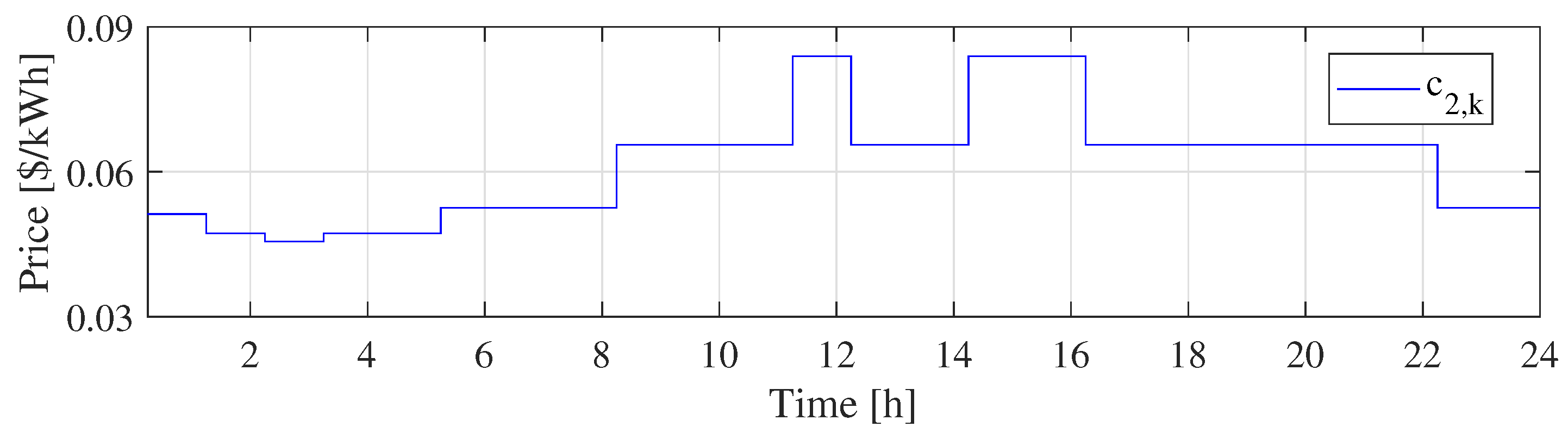
| Energy price 2 (time slot k) | Mean value | ||
| Std dev. | |||
| Remuneration price (time slot k) | , | - |
| EV | EV | EV | EV | EV | EV | EV | EV | EV | EV | EV | |
|---|---|---|---|---|---|---|---|---|---|---|---|
| 28.0 | 23.0 | 32.0 | 13.0 | 23.0 | 17.0 | 22.0 | 26.0 | 24.0 | 18.0 | 30.0 | |
| 8.4 | 21.7 | 17.1 | 7.6 | 6.9 | 3.2 | 3.4 | n/d | 6.6 | 16.3 | 21.5 | |
| n/d | |||||||||||
| n/d | |||||||||||
| ID | 1 | 2 | 3 | 1 | 2 | 3 | 1 | n/a | 1 | 2 | 1 |
| Strategy | Charging | Cost | Capacity | Capacity |
|---|---|---|---|---|
| Cost [$] | Savings [%] | [kWh] | [kWh] | |
| Minimum Time (MT) | − | |||
| economic Model Predictive Control (eMPC) | ||||
| Optimal Control with Minimum Cost and | ||||
| Maximum Flexibility (OCCF) |
| Strategy | Charging | Cost | Capacity | Capacity |
|---|---|---|---|---|
| Cost ($) | Savings (%) | (kWh) | (kWh) | |
| MT | - | |||
| eMPC | ||||
| OCCF |
| Strategy | Charging | Cost | Capacity | Capacity |
|---|---|---|---|---|
| Cost ($) | Savings (%) | (kWh) | (kWh) | |
| MT | 2913.13 | - | 0.0 | 47,600.00 |
| eMPC | 2322.36 | 20.28 | 40,979.68 | 42,620.32 |
| OCCF | 2706.40 | 7.10 | 61,059.26 | 42,240.74 |
| Strategy and | Overall Savings | Strategy and | Overall Savings | ||
|---|---|---|---|---|---|
| Remuneration Factor | Mean (%) | Std (%) | Remuneration Factor | Mean (%) | Std (%) |
| eMPC, | 19.8 | 1.6 | eMPC, | 10.6 | 0.8 |
| OCCF, | 44.5 | 2.1 | OCCF, | 35.3 | 1.3 |
| OCCF, | 59.5 | 2.4 | OCCF, | 53.9 | 2.2 |
| OCCF, | 81.6 | 3.4 | OCCF, | 80.6 | 3.0 |
| OCCF, | 257.9 | 10.2 | OCCF, | 257.9 | 10.1 |
© 2019 by the authors. Licensee MDPI, Basel, Switzerland. This article is an open access article distributed under the terms and conditions of the Creative Commons Attribution (CC BY) license (http://creativecommons.org/licenses/by/4.0/).
Share and Cite
Diaz-Londono, C.; Colangelo, L.; Ruiz, F.; Patino, D.; Novara, C.; Chicco, G. Optimal Strategy to Exploit the Flexibility of an Electric Vehicle Charging Station. Energies 2019, 12, 3834. https://doi.org/10.3390/en12203834
Diaz-Londono C, Colangelo L, Ruiz F, Patino D, Novara C, Chicco G. Optimal Strategy to Exploit the Flexibility of an Electric Vehicle Charging Station. Energies. 2019; 12(20):3834. https://doi.org/10.3390/en12203834
Chicago/Turabian StyleDiaz-Londono, Cesar, Luigi Colangelo, Fredy Ruiz, Diego Patino, Carlo Novara, and Gianfranco Chicco. 2019. "Optimal Strategy to Exploit the Flexibility of an Electric Vehicle Charging Station" Energies 12, no. 20: 3834. https://doi.org/10.3390/en12203834
APA StyleDiaz-Londono, C., Colangelo, L., Ruiz, F., Patino, D., Novara, C., & Chicco, G. (2019). Optimal Strategy to Exploit the Flexibility of an Electric Vehicle Charging Station. Energies, 12(20), 3834. https://doi.org/10.3390/en12203834