PMSM Vector Control Strategy Based on Active Disturbance Rejection Controller

Abstract

Based on current research into the vector control principles of the permanent magnet synchronous motor (PMSM), a control strategy founded upon an Active Disturbances Rejection Controller (ADRC) is proposed. This control strategy consists of an ADRC speed loop and current controller. By studying the factors affecting the running state of a PMSM, a mathematical model is established, and the design principle of the active disturbances rejection controller is analyzed in order to design the ADRC speed loop. The speed loop considers errors caused by uncertain factors, such as external disturbances, to be the disturbance amount, which is observed and then compensated for by the ADRC, thereby improving the dynamic and static performance as well as the anti-disturbance capability of the system. In order to achieve the strong coupling of the PMSM, the current controller was also designed to decouple the d–q axis current. Our simulation and experimental results demonstrate the feasibility and practicability of this control strategy.

1. Introduction

The energy crisis and environmental issues which characterize the early 21st Century have been generating fear and uncertainty worldwide [1]. As awareness grows that our continued reliance upon fossil fuels is untenable, the traditional automotive industry has suffered, and electric vehicles powered by alternative energy have emerged as an increasingly popular alternative [2]. The permanent magnet synchronous motor (PMSM) has been widely promoted within the field of electric vehicles, as it possesses a number of desirable characteristics, including a small torque ripple, a wide speed range, a simple structure, a large torque inertia and low vibration noise [3,4,5]. As the in-depth study of PMSM control systems has progressed, a variety of advanced control strategies have been proposed, including a synovial deformation structure, time optimal control, adaptive control and nonlinear proportional–integral–derivative (PID) [6,7]. However, the control effect of most strategies depends upon the precise model of the controlled object, which is more complicated and difficult to implement. Artificial intelligence control has become a hot topic in current research because of its strong robustness and also remaining independent of the controlled object model. The complexity of the algorithm, and the large amount of computation, limit its application in the actual control system. The PI controller is widely used in the speed loop and current loop of the control system due to its simple structure and easy implementation. But the control performance in the time-varying system is weak, and there are problems such as overshoot, which make it difficult to achieve high-precision control [8,9].

The Active Disturbances Rejection Controller (ADRC) was developed by the researcher Han Jingqing of the Chinese Academy of Sciences following in-depth research into modern control theory [10,11,12,13,14]. It combines PID control technology based on error feedback, using this to eliminate the essence of error control, and thereby proposing a new, nonlinear, practical control method [10,11,12,15]. The ADRC suppresses overshoot by means of the Tracking Differentiator (TD) design transition process during operation, and observes the external disturbance and parameter variation of the system through the Extended State Observer (ESO) [13,14,16]. The ESO accounts for the defects of the PID controller and results in the accelerated convergence of any error, as well as possessing desirable dynamic and static characteristics [17].

This paper investigates the PMSM, and from the analysis of its topology and principles, a control strategy based on an ADRC is proposed. Since the PMSM is a complex nonlinear system, favorable control performance can be obtained by decoupling the coupling term in its mathematical equation. The commonly-used PI control decoupling is difficult to meet the performance requirements in the full speed range. Therefore, the feedback linearization theory is applied. The Lie differential operation of the output variable is used to obtain the required coordinate transformation and nonlinear system state feedback. The input-output feedback linearization of the PMSM is realized, and the feedback linearization algorithm is designed. The controller implements the decoupling control of the system. Our simulation and experimental research into the control system demonstrate that our proposed control strategy is robust, and exhibits both stable and accurate dynamic tracking.

This paper is organized as follows: The design of ADRC is given in Section 2. In Section 3, the current decoupling controller and the magnetic chain observer are given. Section 4 provides simulation and experimental results. Section 5 concludes this paper.

2. The Active Disturbances Rejection Controller

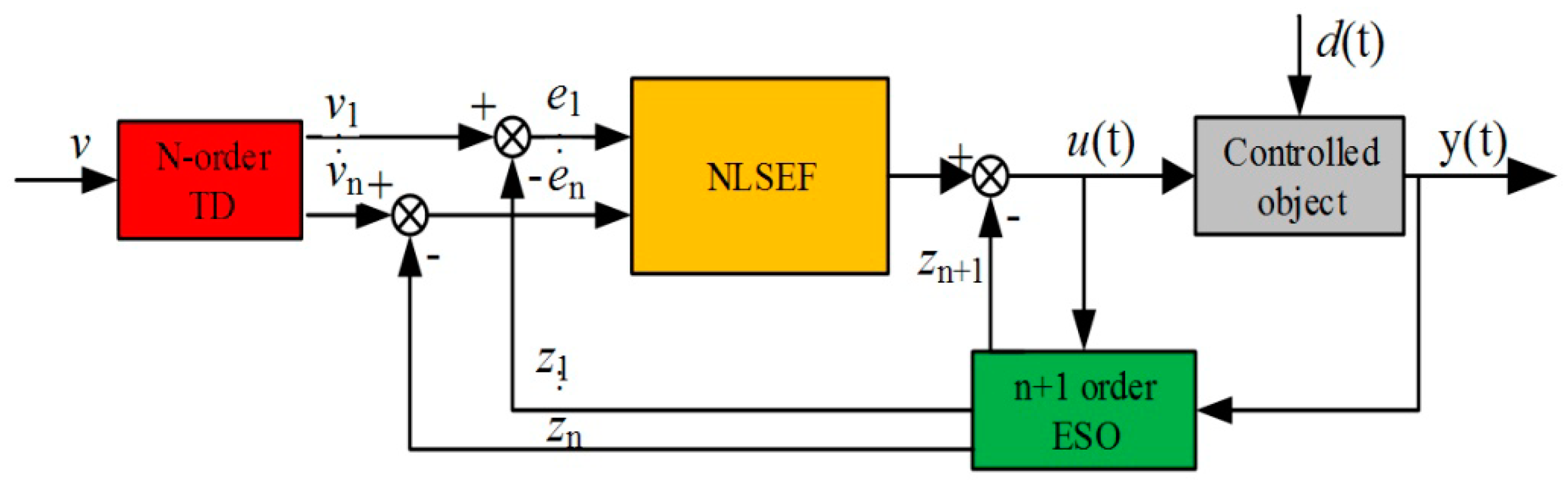
Active disturbances rejection controller technology is a nonlinear control strategy. It combines classical adjustment theory with modern control theory, and has the advantages of simple algorithm and easy adjustment [18]. This control theory applies nonlinear feedback to the control system to compensate for errors caused by uncertainties such as internal and external disturbances. Moreover, the active disturbances rejection controller technology has a low dependence on the accuracy of the mathematical model of the controlled system, so it has unique advantages in dealing with the nonlinear control system. The active disturbances rejection controller mainly includes three parts: The tracking differentiator (TD), extended state observer (ESO) and nonlinear state error feedback (NLSEF) [19].

Since the auto-disturbance technique can be applied to an uncertain object that is affected by an unknown disturbance, it is described by the following differential equation.

$$\{\begin{array}{l}{x}^{(n)}=f(x,\dot{x},\cdots ,x^{(n-1)},t)+d(t)+bu(t)\\ y=x(t)\end{array}$$

(1)

Where: $f(x,\dot{x},\cdots ,x^{(n-1)},t)$ is an unknown function; d(t) is an unknown disturbance; y is the system output; u(t) is the system control quantity; b is the gain of control input.

The schematic diagram of the standard active disturbances rejection controller is shown in Figure 1.

2.1. Tracking Differentiator

The tracking differentiator is the first part of the auto-disturbance controller. The tracking transition process effectively solves the problem that the super-adjustment and rapidity of the classical PID control technology have difficulty in coordinating in the control system, and reduces the overshoot of the system. It enables it to track the system reference input quickly, while obtaining an approximate differential signal according to the order of the controller [20,21,22,23]. The second order differential equation is:

$$\{\begin{array}{l}{\dot{z}}_1=z_2\hfill \\ {\dot{z}}_2=f(z_1,z_2)\hfill \end{array}$$

(2)

All solutions are bounded and satisfied by:

$$\{\begin{array}{c}\underset{t\to \infty }{\lim }{z}_1(t)=0\\ \underset{t\to \infty }{\lim }{z}_2(t)=0\end{array}$$

(3)

For any bounded measurable signal v(t), $t\in \left[0,\infty \right]$ and arbitrary T > 0, differential equation is:

$$\{\begin{array}{l}\dot{x}=x_2\hfill \\ \dot{x}=r^{2}f(x-v(t),\frac{x_2}{r})\hfill \end{array}$$

(4)

The first component of the solution x₁(r, t) is satisfied by:

$$\lim {\displaystyle \int \begin{array}{c}T\\ 0\end{array}}|x1(r,t)-v(t)|dt=0$$

(5)

Extend the above equation to the nth order system, the dynamic system is set up:

$$\{\begin{array}{l}{\dot{z}}_1=z_2\\ ⋮\\ {\dot{z}}_{n-1}=z_n\\ {\dot{z}}_n=f(z_1,z_2,\cdots ,z_n)\end{array}$$

(6)

Where any solution is asymptotically stable at the origin, and all solutions are satisfied by $\lim zi(t)=0,i=1,2,\cdots ,n$. Then, for any locally integrable signal v(t), with $t\in [0,\infty )$, and any T > 0, the new dynamic system for any bounded integrable function v(t) is:

$$\{\begin{array}{l}{\dot{x}}_1=x_2\\ ⋮\\ {\dot{x}}_{n-1}=x_n\\ {\dot{x}}_n=r^{n}f(x_1-v(t),\frac{x_2}{r},\cdots \frac{x_n}{r^{n-1}})\end{array}$$

(7)

Solution satisfies: $\underset{r\to \infty }{\lim }{\displaystyle {\int }_0^T|x_1(t)-v(t)|}dt=0$. As r increases, the system solution can fully approximate a given input signal for a limited time.

2.2. Extended State Observer

The system always exchanges information with the environment during its operation. For a dynamic system, the external variable of the system is the output variable of the system to the outside. The device that determines the state variable inside the system according to the observation of the external variable is the state observer, and it determines the system according to the measured system input and system output. The extended state observer is, in a sense, a versatile and applicable disturbance observer.

Set the second-order linear control system as:

$$\{\begin{array}{l}{\dot{x}}_1=x_2\hfill \\ {\dot{x}}_2=a_1{x}_1+a_2{x}_2+bu\hfill \\ y=x_1\hfill \end{array}$$

(8)

The corresponding system state observer is:

$$\{\begin{array}{l}{e}_1=z_1-y\hfill \\ {\dot{z}}_1=z_2-l_1{e}_1\hfill \\ {\dot{z}}_2=(a_1{z}_1+a_2{z}_2)-l_2{e}_1+bu\hfill \end{array}$$

(9)

The error equation between the system and the original system is:

$$\{\begin{array}{l}{e}_1=z_1-x_1,e_2=z_2-x_2\hfill \\ {\dot{e}}_1=-l_1{e}_1+e_2\hfill \\ {\dot{e}}_2=(-l_2+a_1)e_1+a_2{e}_2+bu\hfill \end{array}$$

(10)

Select l₁, l₂ to make matrix $\left[\begin{array}{cc}-l_1& 1\\ -l_2& a_2\end{array}\right]$ stable; the Equation (9) is the state observer of the Equation (8).

Nonlinear system is:

$$\{\begin{array}{l}{\dot{x}}_1=x_2\hfill \\ {\dot{x}}_2=f(x_1,x_2)+bu\hfill \\ y=x_1\hfill \end{array}$$

(11)

When f(x₁, x₂) and b are determined, the following state observer is established:

$$\{\begin{array}{l}{e}_1=z_1-y\hfill \\ {\dot{z}}_1=z_2-l_1{e}_1\hfill \\ {\dot{z}}_2=f(z_1,z_2)-l_2{e}_1+bu\hfill \end{array}$$

(12)

The error equation for the Equation (12) is:

$$\{\begin{array}{l}{e}_1=z_1-x_1,e_2=z_2-x_2\hfill \\ {\dot{e}}_1=e_2-l_1{e}_1\hfill \\ {\dot{e}}_2=f(x_1+e_1,x_2+e_2)-f(x_1,x_2)-l_2{e}_1\hfill \end{array}$$

(13)

Assuming that f(x₁, x₂) is continuously differentiable, it is linearly approximated by a Taylor expansion:

$$\{\begin{array}{l}{e}_1=z_1-x_1,e_2=z_2-x_2\hfill \\ {\dot{e}}_1=e_2-l_1{e}_1\hfill \\ {\dot{e}}_2=\frac{\partial f(x_1,x_2)}{\partial x_1}e1+\frac{\partial f(x_1,x_2)}{\partial x_2}{e}_2-l_2{e}_1\hfill \end{array}$$

(14)

As long as $\frac{\partial f(x_1,x_2)}{\partial x_1}$ and $\frac{\partial f(x_1,x_2)}{\partial x_2}$ are bounded, l₁ and l₂ can always be determined, and if the error Equation (14) is stable, Equation (12) will become the state observer of the Equation (11).

Define $x_3(t)=f(x_1(t),x_2(t))$ and ${\dot{x}}_3(t)=w(t)$, then Equation (11) can be expanded into a new linear control system:

$$\{\begin{array}{l}{\dot{x}}_1=x_2\hfill \\ {\dot{x}}_2=x_3+bu\hfill \\ {\dot{x}}_3=w(t)\hfill \\ y=x_1\hfill \end{array}$$

(15)

Establish a state observer for the expanded system:

$$\{\begin{array}{l}{e}_1=z_1-y\hfill \\ {\dot{z}}_1=z_2-{\beta }_1{e}_1\hfill \\ {\dot{z}}_2=z_3-{\beta }_2{|e_1|}^{\frac{1}{2}}sign(e_1)+bu\hfill \\ {\dot{z}}_3=-{\beta }_3{|e_1|}^{\frac{1}{4}}sign(e_1)\hfill \end{array}$$

(16)

By selecting the appropriate parameters β₁, β₂ and β₃, the system can estimate the state variables x₁(t) and x₂(t) and the real-time effect x₃(t) of the expanded state. The state observer of the expanded Equation (16) is called the state observer, and x₃(t) is called the expanded state.

The extended state observer obtains the tracking signal z₁(t) of the system output signal y(t) and the derivative signal z_i(t) of each order, and the system disturbance estimation signal z_n+1(t) to estimate the disturbance. Extend the external disturbance and model error to a new state variable. According to the classical state observer principle, the following equation can be obtained:

$$\{\begin{array}{l}e=z_1-y\\ {\dot{z}}_1=z_2+g_1(e)\\ ⋮\\ {\dot{z}}_{n-1}=f(x_1,\cdots ,x_{n-1})+bu+g_{n-1}(e)\\ {\dot{z}}_n=g_n(e)\end{array}$$

(17)

Select the appropriate function to observe the state variables and total disturbances of the system.

2.3. Nonlinear State Error Feedback Controller

The nonlinear structure and control parameters play a key role in the fast convergence of the auto disturbance rejection controller to the target. “Feedback” is the essence of control theory. The feedback mechanism can improve the performance of the system. It can change a linearly-controlled system into a nonlinear-controlled system, and vice versa. The feedback mechanism in the negative feedback-controlled system also has the ability to restrain small, uncertain disturbances. The most breakthrough idea of self-disturbance control is to explore the potential of the feedback mechanism as much as possible, and to exert its control and anti-interference ability.

The tracking differentiator and the extended state observer respectively generate tracking signals and state variables. The nonlinear state error feedback controller uses a function to solve the control quantity structure by using the functions of the above two parameters.

The general form is as follows:

$$\{\begin{array}{l}{e}_1=v_1-z_1\\ ⋮\\ e_n=v_n-z_n\\ u_0(t)=k_1{f}_1(e_1,t)+\cdots +k_n{f}_n(e_n,t)\\ u(t)=u_0(t)-z_{n+1}(t)/b\end{array}$$

(18)

Where: e_i(i = 1,2,...,n) is the difference between the tracking signal and the state variable estimate; f_i(e_i, t) is a nonlinear function; u₀(t) is the system control quantity; −z_{n + 1}(t)/b acts to compensate for the disturbance.

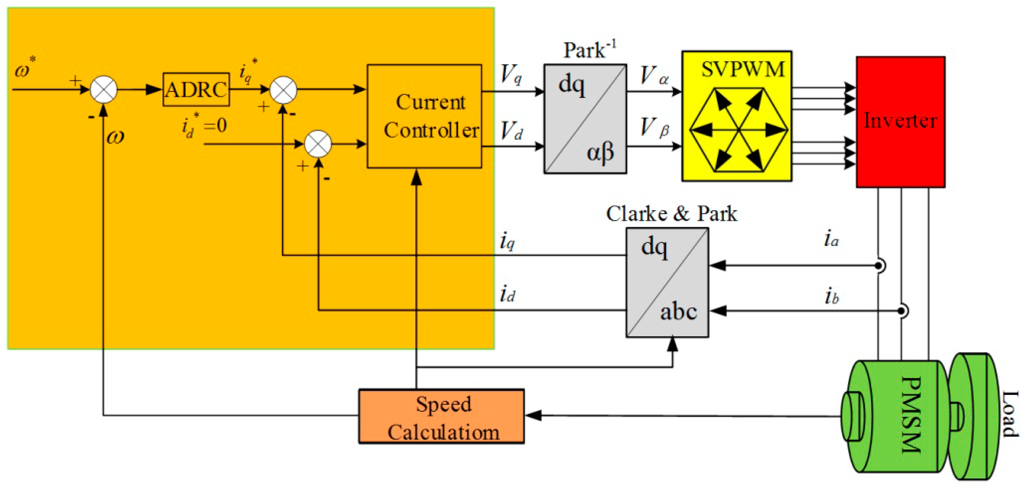
3. Design of ADRC

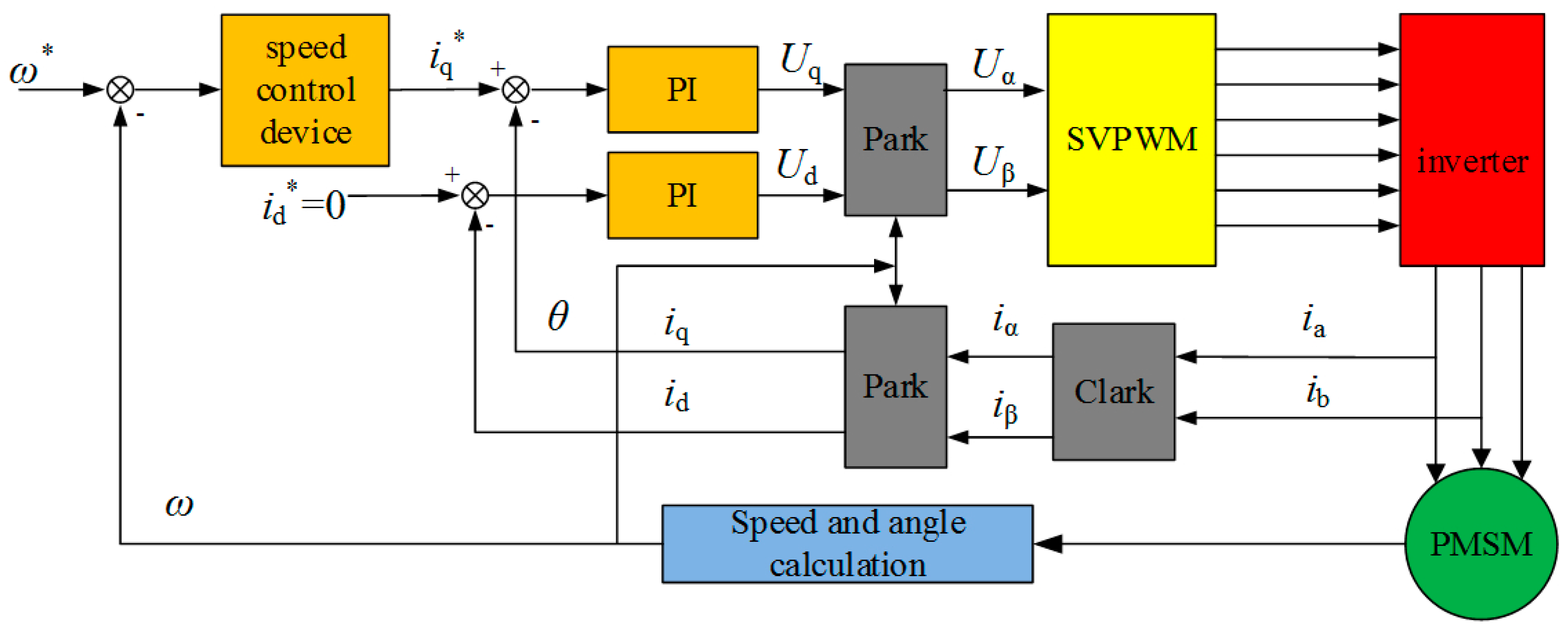
The classic permanent magnet synchronous motor i_d* = 0 vector control strategy usually adopts the double loop control structure, where the inner loop is the current loop, and the outer loop is the speed loop. At this time, the principle structure diagram of the vector control speed control system of the permanent magnet synchronous motor based on i_d* = 0 is shown in Figure 2 [23,24,25,26].

In order to facilitate the analysis and application, the interference of the core parameters, such as core saturation, higher harmonics and eddy current on the motor parameters, is temporarily ignored. The voltage equation of the PMSM in the synchronous rotating coordinate system is as follows:

$$u_d=R_s{i}_d+\frac{d}{dt}{\psi }_d-{\omega }_e{\psi }_q$$

(19)

$$u_q=R_s{i}_q+\frac{d}{dt}{\psi }_q+{\omega }_e{\psi }_d$$

(20)

The flux linkage equation is:

$${\psi }_d=L_d{i}_d+{\psi }_f$$

(21)

$${\psi }_{\mathrm{q}}=L_{\mathrm{q}}{i}_q$$

(22)

Based upon the theory of magnetic field orientation, the state equation of a PMSM in a synchronous rotating coordinate system is [27]:

$$\left[\begin{array}{l}{\dot{i}}_d\\ {\dot{i}}_q\\ {\dot{\omega }}_e\end{array}\right]=\left[\begin{array}{ccc}-R_s/L& n_p{\omega }_e& 0\\ n_p{\omega }_e& -R_s/L& -n_p{\psi }_f/L\\ 0& 1.5n_p{\psi }_f/J& -B/J\end{array}\right]\left[\begin{array}{c}{i}_d\\ i_q\\ {\omega }_e\end{array}\right]+\left[\begin{array}{c}{u}_d/L_d\\ u_q/L_q\\ -T_L/J\end{array}\right]$$

(23)

Where u_d, u_q, ψ_d, and ψ_q are the stator voltage and flux linkage components in the d–q coordinate system, respectively, and also where i_d and i_q are the direct axis and the intersecting axis current, respectively; L_d is the direct axis and L_q the intersecting axis inductance. Meanwhile, R_s is the stator resistance; ψ_f is the rotor flux; T_L is the load torque; P_n is the motor pole pair; J is the moment of inertia; and ω_e is the rotor angular velocity.

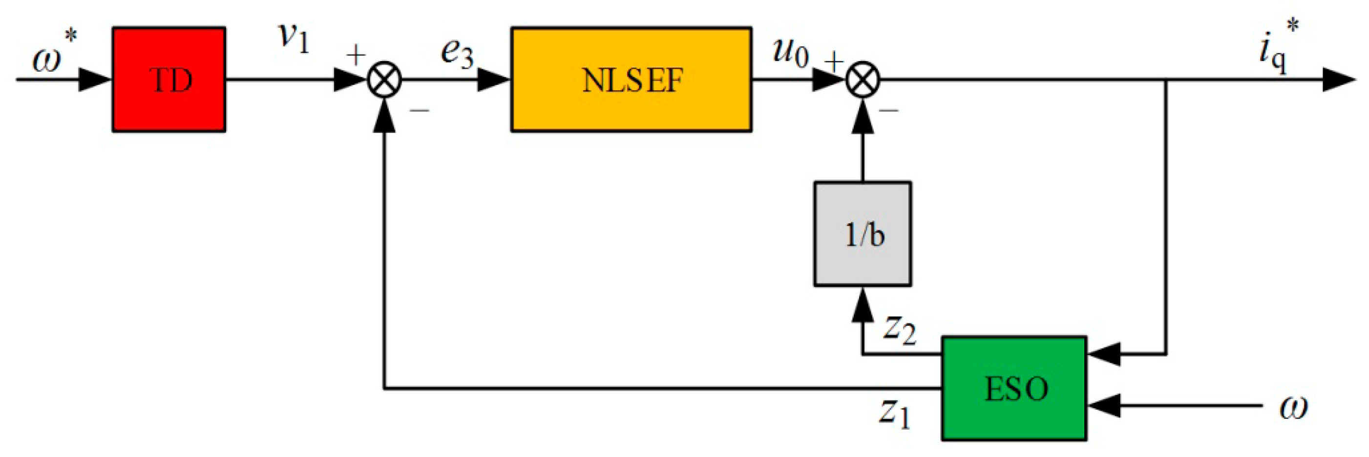
From the design of the auto-disturbance controller on the speed loop, the system state is only the speed. Therefore, only one-order ADRC is needed for this factor, so that the extended state observer is the second-order. In order to facilitate control and reduce the number of controlled parameters, a linear function is used instead of a nonlinear function.

From Equation (23), we can get:

$${\dot{\omega }}_e=\frac{3n_p{\psi }_f{i}_q}{2J}-\frac{B{\omega }_e}{J}-\frac{T_L}{J}$$

(24)

Set the disturbance:

$$a(t)=-\frac{B}{J}{\omega }_e-\frac{T_L}{J}$$

(25)

$$b=1.5\frac{n_p{\psi }_f}{J}$$

(26)

Inferred:

$$\dot{\omega }=a(t)+b{i}_q$$

(27)

It can be seen from the above equation that the motion damping coefficient, moment of inertia and external disturbance of the PMSM can be represented in a(t). Consequently, the transition should be arranged in a manner that achieves the real-time tracking of the input signal. At the same time, in order to improve the anti-disturbance ability of the system, a(t) should be observed and compensated for. Therefore, the specific structure of the first-order ADRC controller, designed according to the principle of active disturbance rejection, is shown in Figure 3.

First-order tracking differentiator:

TD:

$$\{\begin{array}{l}{e}_1=v_1-{\omega }^{*}\\ {\dot{v}}_1=-r{e}_1\end{array}$$

(28)

ESO:

$$\{\begin{array}{l}{e}_1=z_1-\omega \\ {\dot{z}}_1=z_2-{\beta }_1{e}_2+bu\\ {\dot{z}}_2=-{\beta }_2{e}_2\end{array}$$

(29)

NLSEF:

$$\{\begin{array}{l}{e}_3=v_1-z_1\\ u_0=k{e}_3\\ u=u_0-\frac{z_2}{b}\end{array}$$

(30)

Where: ω* is the given speed variable; v₁ is the tracking signal; ω is the actual motor speed; z₁ is the observed signal; z₂ is the disturbance feedback.

It can be seen from the above equations that there are r, β₁, β₂ and k in the ADRC control system which are need to be set. It can be seen from Equation (28) that increasing the parameter r in the tracking differentiator can bring the tracking signal closer to a given speed. However, overshoot will occur as r increases, so multiple tunings are required. β₁, and β₂ determine the performance of ESO, which is mainly reflected in the convergence speed. β₂ affects the estimation of disturbances in the ESO system. As the value increases, the system’s load-resistance is enhanced. Therefore, the time for the system to return to steady state after the sudden change of the load is short. However, the system oscillation is more obvious when β₂ is over-exposed, so β₁ is increased to restrain the oscillation at this time.

According to the method proposed by Gao Zhiqiang, the system bandwidth and the extended state observer bandwidth are used to reduce the number of tuning parameters. Using the linear system synthesis method to perform pole assignment on Equation (29), we can derive the characteristic equation as:

$$p(s)=s^2+{\beta }_{1}s+{\beta }_2$$

(31)

The necessary and sufficient condition for β₁ and β₂ is that all of the roots of Equation (18) must be on the left plane. If a closed-loop pole is desired $-p(p>0)$, then:

$$p(s)={(s+p)}^2=s^2+2ps+p^2$$

(32)

By using system bandwidth ω_c and extended state observer bandwidth ω₀, the observation poles can be placed on top ω₀:

$${\beta }_1=2{\omega }_0,{\beta }_2={\omega }_0{}^2$$

(33)

$${\omega }_0\approx 3~5{\omega }_c$$

(34)

Only one parameter needs to be set. The larger the tracking signal, the faster the system response. In the experiment, the trial-and-error method was used to adjust the system parameters. In short, the tuning of the four parameters should be coordinated and adjusted. Through the experience and comparative analysis of each simulation, multiple attempts are made to determine the most appropriate parameters.

The pole placement method is currently a widely-used parameter tuning method. It is simple and easy to use, and the parameters are satisfied within a certain range.

4. Current Controller Design

The current controller mainly comprises a current decoupling controller and a flux linkage observer. The decoupling controller applies the feedback linearization theory to decouple the complex coupling terms in the mathematical equations of the motor. The flux observer provides the necessary information for the decoupling controller.

4.1. Current Decoupling Controller

Because the electromagnetic torque of the three-phase permanent magnet synchronous motor is:

$$T_e=1.5p_n({\psi }_d{i}_q-{\psi }_q{i}_d)$$

(35)

Where: T_e is the electromagnetic torque.

Substituting Equations (21) and (22) into Equation (31) yields:

$$T_{\mathrm{e}}=1.5p_n[{\psi }_f{i}_q+(L_d-L_q)i_d{i}_q]$$

(36)

Since L_d = L_q = L, Equation (32) can be simplified as:

$$T_e=1.5n_p{\psi }_f{i}_q$$

(37)

It can be seen from Equation (23) that the PMSM is a multi-variable system. There is a strong nonlinear coupling relationship between i_d, i_q and ω_e, which cannot be adjusted separately. Therefore, i_d and i_q need to be used in order to achieve decoupling.

A rewriting of the system state Equation (23) in the d–q coordinate system to the affine nonlinear standard form is as follows:

$$\dot{x}=f(x)+g_1(x)u_d+g_2(x)u_q$$

(38)

$$f(x)=\left[\begin{array}{l}-R_S{i}_d+L_q{i}_q{\omega }_e\hfill \\ -R_S{i}_q-L_d{i}_d{\omega }_e-{\omega }_e{\psi }_f\hfill \\ (T_e-P_n{T}_L-B{\omega }_e)/J\hfill \end{array}\right]$$

(39)

$$\left[\begin{array}{cc}{g}_1(x)& g_2(x)\end{array}\right]=\left[\begin{array}{cc}1& 0\\ 0& 1\\ 0& 0\end{array}\right]$$

(40)

Before the controller can be designed, the conditions under which the feedback linearization method is established in the direct torque control system must be discussed.

$$\begin{array}{c}\left[\begin{array}{cc}{L}_{g_1}{\psi }_d& L_{g_2}{\psi }_d\\ L_{g_1}{\psi }_q& L_{g_2}{\psi }_q\end{array}\right]=\left[\begin{array}{cc}{g}_1\frac{\partial {\psi }_d}{\partial x}& g_2\frac{\partial {\psi }_d}{\partial x}\\ g_1\frac{\partial {\psi }_q}{\partial x}& g_2\frac{\partial {\psi }_q}{\partial x}\end{array}\right]\\ =\left[\begin{array}{cc}1& 0\\ 0& 1\end{array}\right]\end{array}$$

(41)

The decoupling matrix is a nonsingular matrix that satisfies exact linearization conditions.

To decouple the equations, two virtual control quantities K₁ and K₂ are designed and defined as follows:

$$\{\begin{array}{l}{k}_1={\dot{y}}_1=L_f{\psi }_d+L_{g_1}{\psi }_d{u}_d+L_{g_2}{\psi }_d{u}_q\hfill \\ k_2={\dot{y}}_2=L_f{\psi }_q+L_{g_1}{\psi }_q{u}_d+L_{g_2}{\psi }_q{u}_q\hfill \end{array}$$

(42)

Where: y₁ = ψ_d and y₂ = ψ_q. They are system output variables, where L_fψ_d is the Li derivative of ψ_d with respect to f, and the meanings of L_g1 and L_g2 are similar, and will not be described again.

Bringing Equations (37) and (38) into Equation (34) yields:

$$\left[\begin{array}{l}{u}_d\hfill \\ u_q\hfill \end{array}\right]={\left[\begin{array}{cc}{L}_{g_1}{\psi }_d& L_{g_2}{\psi }_d\\ L_{g_1}{\psi }_q& L_{g_2}{\psi }_q\end{array}\right]}^{-1}\left[\begin{array}{l}{k}_1-L_f{\psi }_d\hfill \\ k_2-L_f{\psi }_q\hfill \end{array}\right]$$

(43)

In order for the changed linear system outputs ψ_d, ψ_q to track the given signals ψ_d* and ψ_q*, the controller is designed to:

$$\{\begin{array}{l}{k}_1=\frac{d{\psi }_d{}^{*}}{dt}-{\alpha }_1\left({\psi }_d{}^{*}-{\psi }_d\right)\hfill \\ k_2=\frac{d{\psi }_q{}^{*}}{dt}-{\alpha }_2\left({\psi }_q{}^{*}-{\psi }_q\right)\hfill \end{array}$$

(44)

Where: α₁ and α₂ are controller modulation parameters with positive values. Finished, u_d and u_q can be expressed as:

$$\{\begin{array}{l}{u}_d=-R{i}_d+{\omega }_e{L}_q{i}_q-k_1\hfill \\ u_q=-R{i}_q-{\omega }_e{L}_d{i}_d+{\omega }_e{\psi }_f-k_2\hfill \end{array}$$

$$\{\begin{array}{l}{u}_d=-R{i}_d+{\omega }_e{L}_q{i}_q-k_1\hfill \\ u_q=-R{i}_q-{\omega }_e{L}_d{i}_d+{\omega }_e{\psi }_f-k_2\hfill \end{array}$$

(45)

And the flux linkage tracking error equation:

$$\{\begin{array}{l}\frac{d\left({\psi }_d{}^{*}-{\psi }_d\right)}{dt}=-{\alpha }_1\left({\psi }_d{}^{*}-{\psi }_d\right)\hfill \\ \frac{d\left({\psi }_q{}^{*}-{\psi }_q\right)}{dt}=-{\alpha }_2\left({\psi }_q{}^{*}-{\psi }_q\right)\hfill \end{array}$$

(46)

It can be seen from these equations that the system’s steady state error can be reduced to be close to zero by making the controller modulation parameter greater than zero.

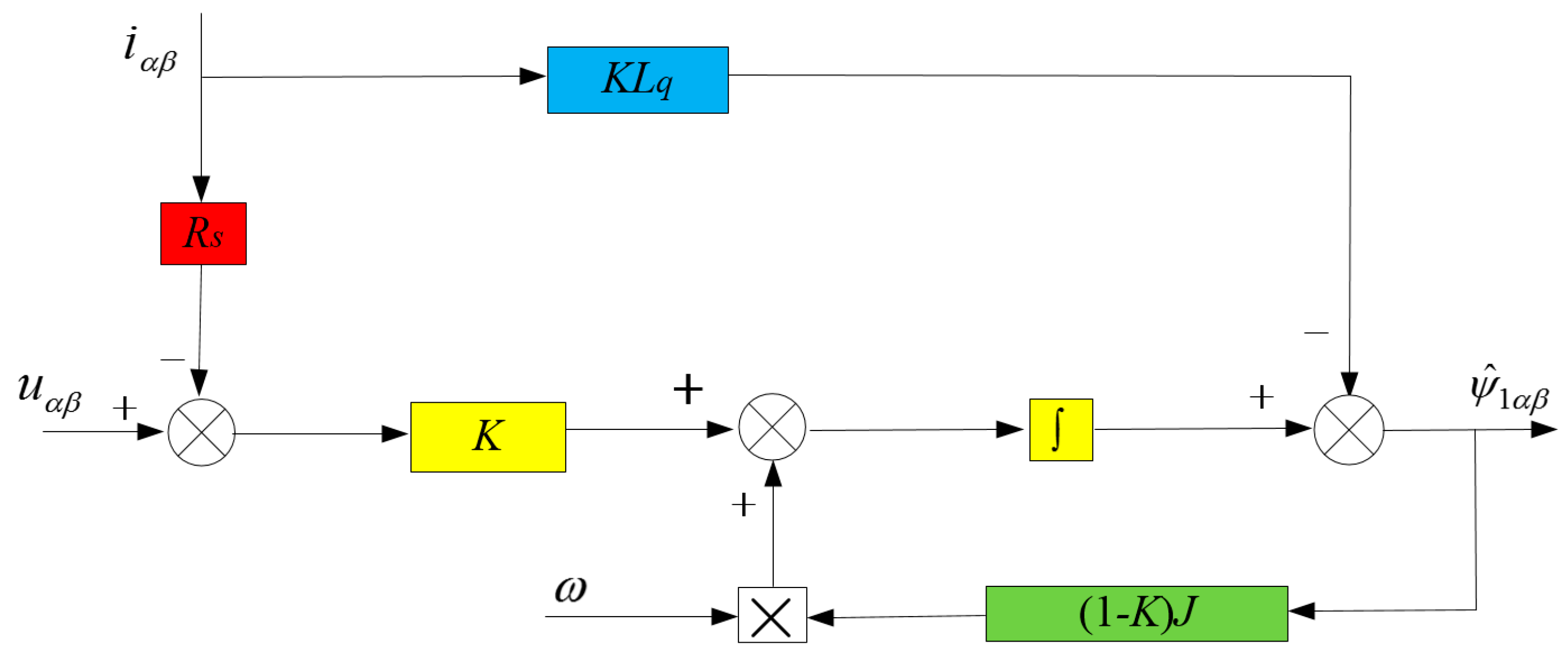
4.2. Magnetic Chain Observer

In order to facilitate the observation of the stator flux linkage, it is necessary to rewrite Equations (19) and (20) into a form under the α–β coordinate system. The mathematical model of the permanent magnet synchronous motor in the α–β coordinate system is:

$$\{\begin{array}{l}{u}_{\alpha }=(R+Dl)i_{\alpha }-{\omega }_e{\psi }_f\sin \theta \hfill \\ u_{\beta }=(R+DL)i_{\beta }+{\omega }_e{\psi }_f\cos \theta \hfill \end{array}$$

(47)

Where D is a differential operator, θ is the rotor flux point angle, and ω_e is the electrical angular velocity.

Construct extended flux linkage terms ψ_α1 and ψ_β1:

$$\{\begin{array}{l}{u}_{\alpha 1}={\psi }_f\cos \theta \hfill \\ u_{\beta 1}={\psi }_f\sin \theta \hfill \end{array}$$

(48)

The extended flux linkage term is used to represent the permanent magnet synchronous motor model:

$$\{\begin{array}{l}{u}_{\alpha }=(R+Dl)i_{\alpha }+D{\psi }_{\alpha 1}\hfill \\ u_{\beta }=(R+DL)i_{\beta }+D{\psi }_{\beta 1}\hfill \end{array}$$

(49)

Order $x={\psi }_{\alpha \beta 1}={\left[\begin{array}{cc}{\psi }_{\alpha 1}& {\psi }_{\beta 1}\end{array}\right]}^T$, a new equation of state is available:

$$\{\begin{array}{l}\dot{x}=Ax+Bu\hfill \\ y=Cx\hfill \end{array}$$

(50)

$$\{\begin{array}{l}A={\omega }_{e}J=\left[\begin{array}{cc}0& -{\omega }_e\\ {\omega }_e& 0\end{array}\right]\hfill \\ B=O=\left[\begin{array}{cc}0& 0\\ 0& 0\end{array}\right]\hfill \\ C={\omega }_{e}J=\left[\begin{array}{cc}0& -{\omega }_e\\ {\omega }_e& 0\end{array}\right]\hfill \end{array}$$

(51)

The relationship between the stator flux linkage and the extended flux linkage is:

$$\{\begin{array}{l}{\psi }_{\alpha }=L{i}_{\alpha }+{\psi }_{\alpha 1}\hfill \\ {\psi }_{\beta }=L{i}_{\beta }+{\psi }_{\beta 1}\hfill \end{array}$$

(52)

The electromagnetic torque equation is:

$$T_e=1.5p_n\left[\begin{array}{cc}{\psi }_{\alpha }& {\psi }_{\beta }\end{array}\right]J^T{\left[\begin{array}{cc}{i}_{\alpha }& i_{\beta }\end{array}\right]}^T$$

(53)

The output y of the system can be measured, so the minimum-order state observer is designed to observe the extended flux linkage. The observer model is:

$$\dot{\widehat{x}}=A\dot{x}+Bu+K[y-\widehat{y}]$$

(54)

Where: K is the state observer feedback matrix. The state observer is constructed according to the state equation, and the state variable is selected as the extended flux linkage ψ_αβ1.

$$\{\begin{array}{l}x={\psi }_{\alpha \beta 1}\hfill \\ \dot{x}=D{\psi }_{\alpha \beta 1}\hfill \end{array}$$

(55)

According to the above formula, the minimum-order state observer of the extended flux linkage is:

$$\{\begin{array}{l}\begin{array}{l}\dot{\widehat{x}}=D{\widehat{\psi }}_{\alpha \beta 1}\\ \hspace{1em}=\widehat{y}+K(y-\widehat{y})\\ \hspace{1em}={\omega }_{e}J{\widehat{\psi }}_{\alpha \beta 1}+K(u_{\alpha \beta }-R_s{i}_{\alpha \beta }-LD{i}_{\alpha \beta }-\omega J{\widehat{\psi }}_{\alpha \beta 1})\end{array}\hfill \\ \widehat{y}={\omega }_{e}J\widehat{x}={\omega }_{e}J{\widehat{\psi }}_{\alpha \beta 1}\hfill \end{array}$$

(56)

The error equation for the state observer is:

$$\begin{array}{ll}D{\tilde{\psi }}_{\alpha \beta 1}& =(A-KC)(\widehat{x}-x)\\ & =\omega (1-K)J({\widehat{\psi }}_{\alpha \beta 1}-{\psi }_{\alpha \beta 1})\end{array}$$

(57)

Where: ${\tilde{\psi }}_{\alpha \beta 1}$ is used to expand the observation error of the observation flux linkage.

It can be seen from the above formula that by performing pole placement on the feedback matrix K, the state observer based on the extended flux linkage can be converged, and the convergence speed is guaranteed to be within a reasonable range. The control block diagram of the extended flux observer is shown in Figure 4:

The system structure block diagram as shown in Figure 5:

5. System Simulation Experiment

During the simulation and testing of the system, the parameters of the PMSM are shown in

Table 1. PMSM parameters.

Parameter	Value
Rated power/(kW)	1.28
Rated speed/(r/min)	2000
Rated torque/(N·m)	75
Polar logarithm	4
Moment of inertia/(kg·m2)	1.469 × 10−3
Ld, Lq/(H)	0.00334
Permanent magnet flux linkage/(Wb)	0.171

, and the parameters of the controller are shown in

Table 2. Controller parameter.

Parameter	Value
r	2 × 106
ω0	1400
β1	2800
β2	1.69 × 106
k	0.6
b	698.4
α1	4720
α2	1910

.

The simulation experiment is carried out under ideal conditions, it mainly includes speed loop and current loop.

Simulation of the speed loop:

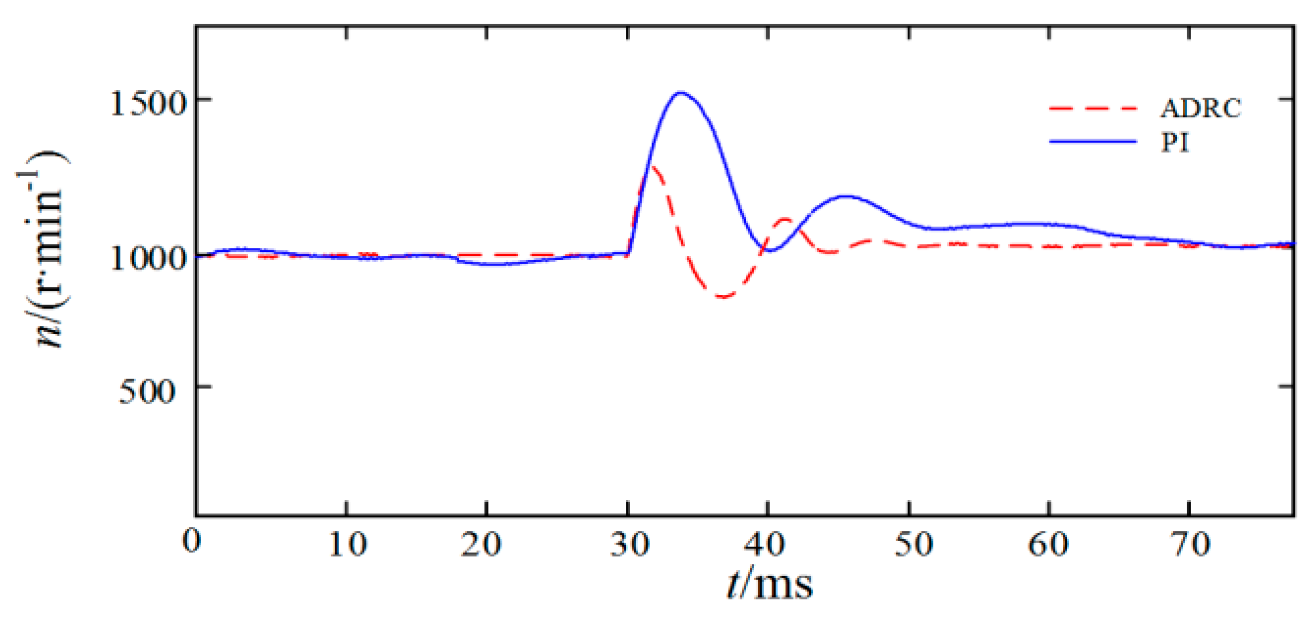
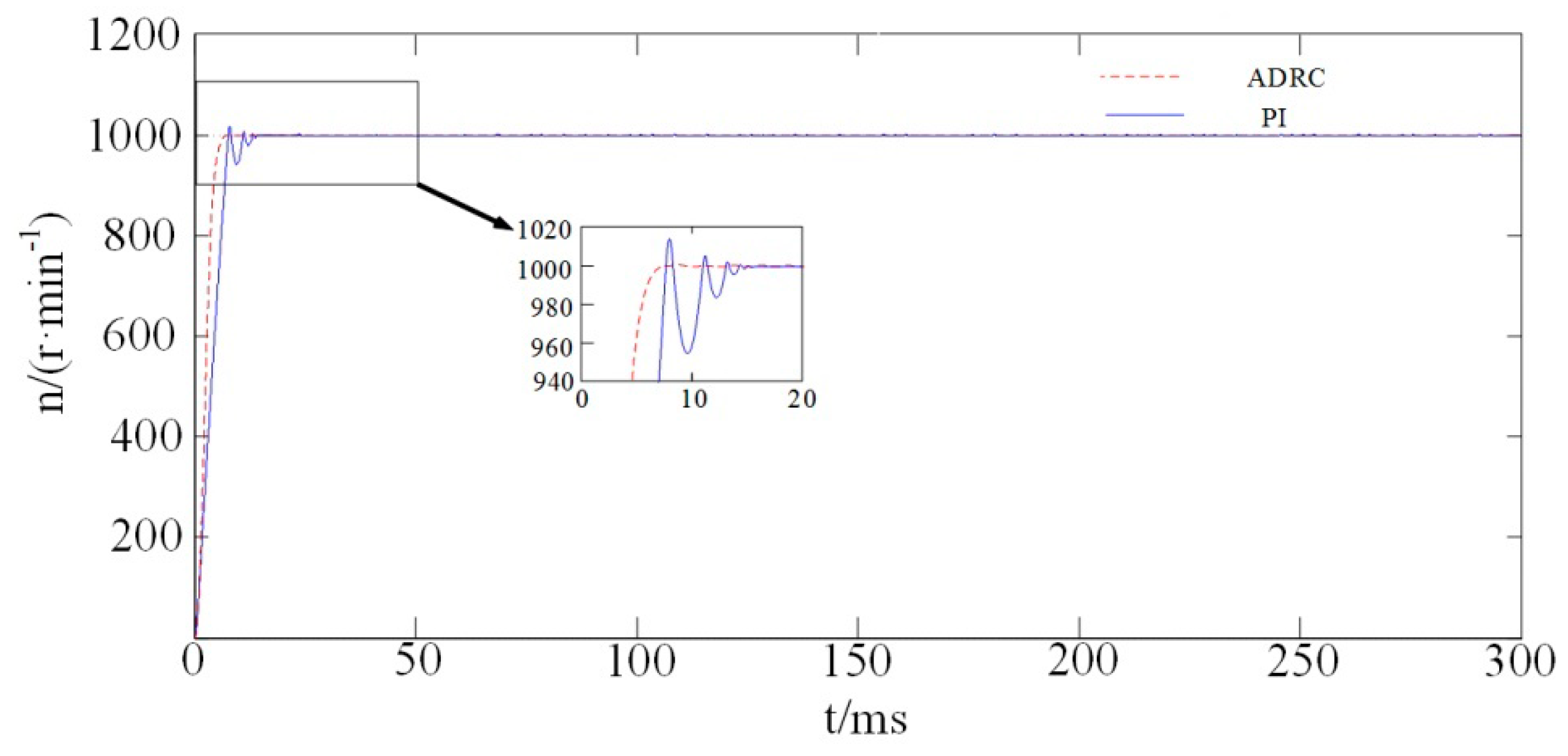
(a) When the speed is n = 1000 r/min, the no-load starts and no disturbance is recorded during the entire process.

Figure 6 reveals that the speed waveform has obvious overshoot when using the PI controller. Additionally, oscillation is significant during the initial stage of the motor starting, and the transition time is long; meanwhile the ADRC controller has no overshoot, a short transition time, and quick response. In short, the motor starts smoothly.

(b) When the speed n = 1000 r/min, the no-load starts, and the torque rises to 2 N·m when t = 30 ms.

(c) When the speed n = 1000 r/min, the torque drop of the 2 N·m torque start at t = 30ms is equal to 0 N·m.

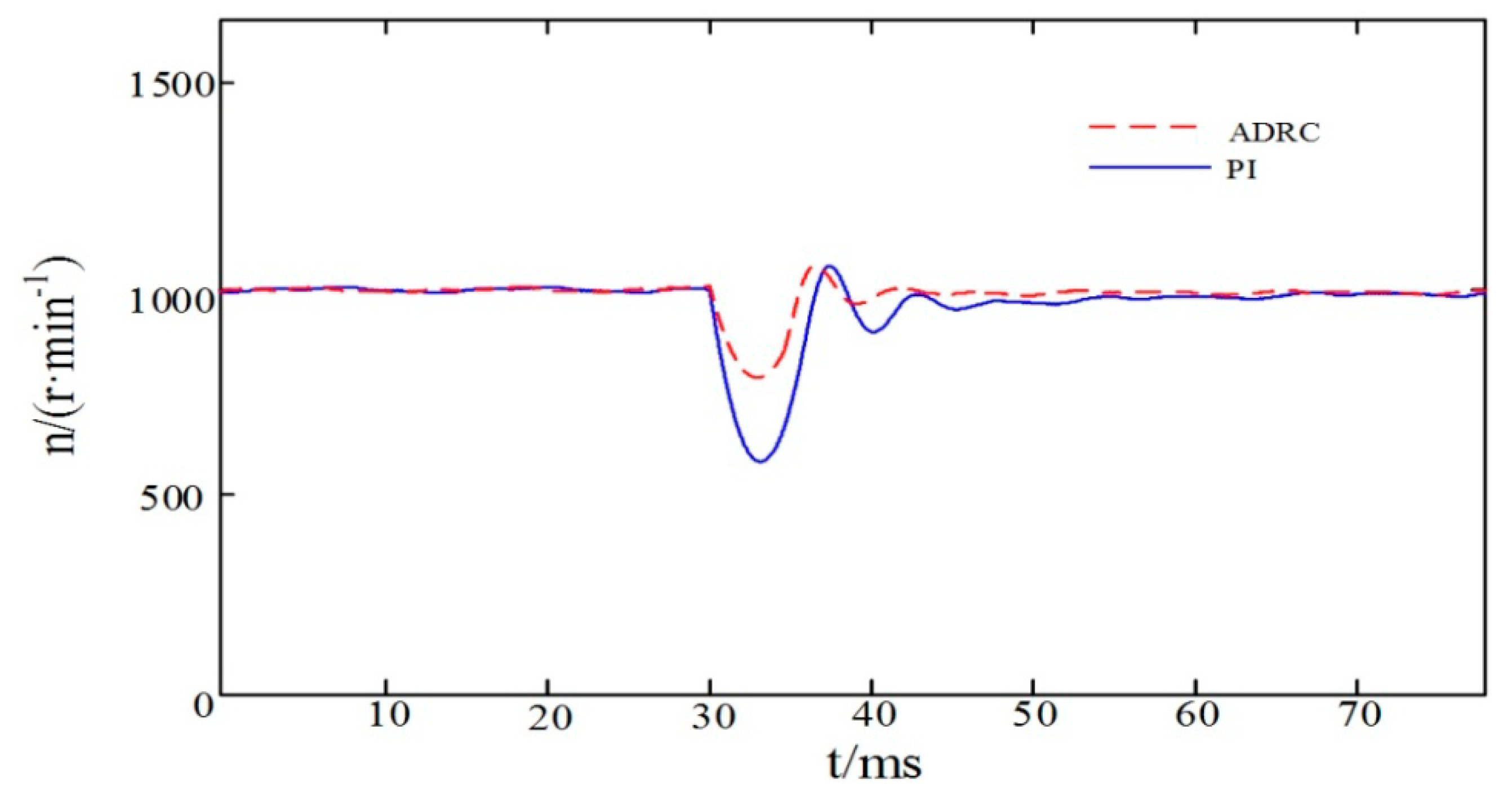
The simulation of the anti-disturbance performance of the ADRC and PI controller are recorded in Figure 7 and Figure 8. As shown, when the load is applied or reduced after the motor is running in a stable manner, the dynamic effect of the ADRC controller speed waveform is superior to that of the PI controller. The advantage is in the fact that the ADRC is shorter than the PI following the disturbance to the steady state, meaning that the change in the rotational speed caused by the sudden alteration of the load is small, resulting in stronger anti-disturbance capabilities.

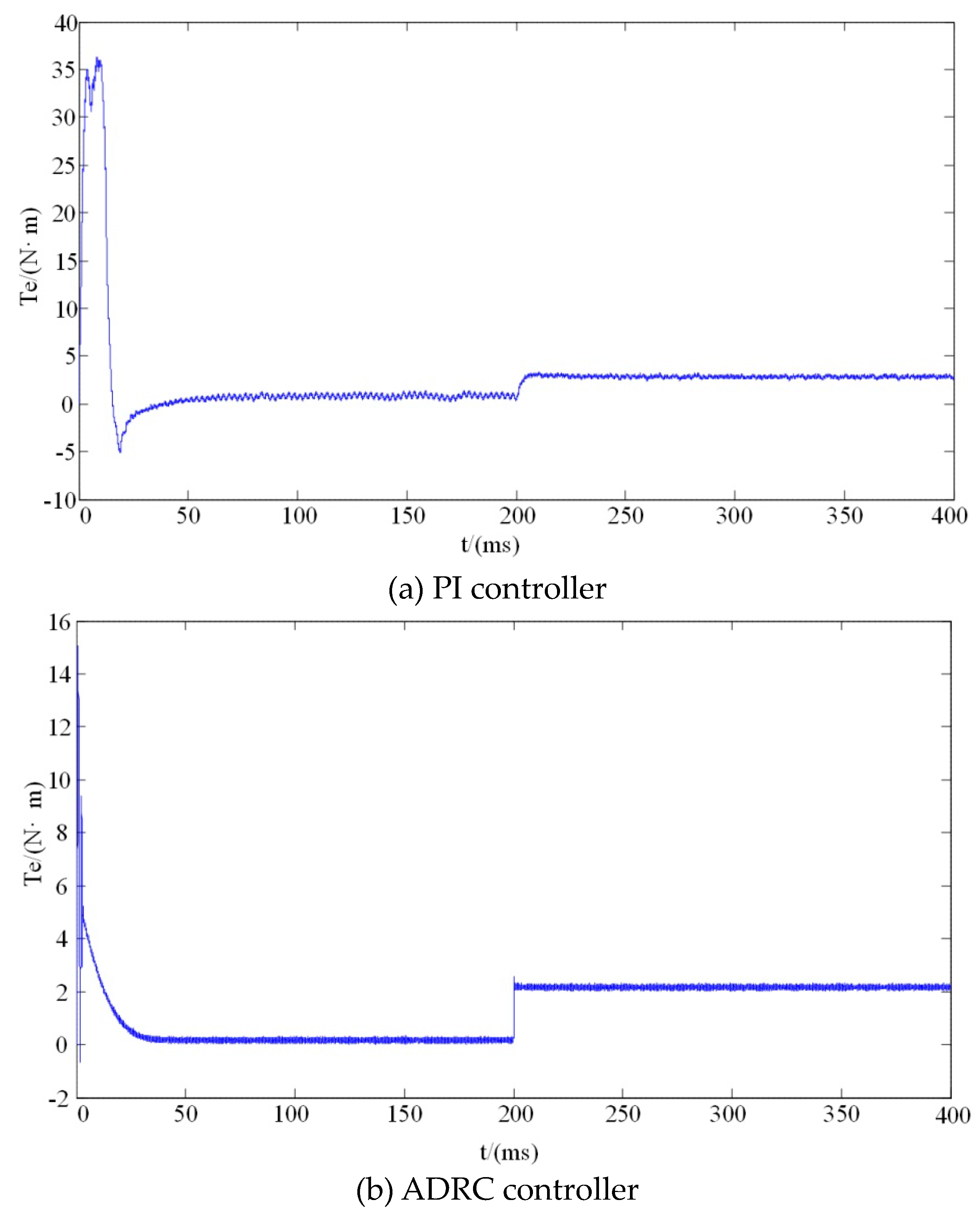
(d) When the rotational speed n = 1000 r/min, the electromagnetic torque waveform is shown in Figure 9. It can be seen from the figure that its starting torque overshoot is smaller, and the transition is faster when the load is suddenly applied.

Current loop simulation:

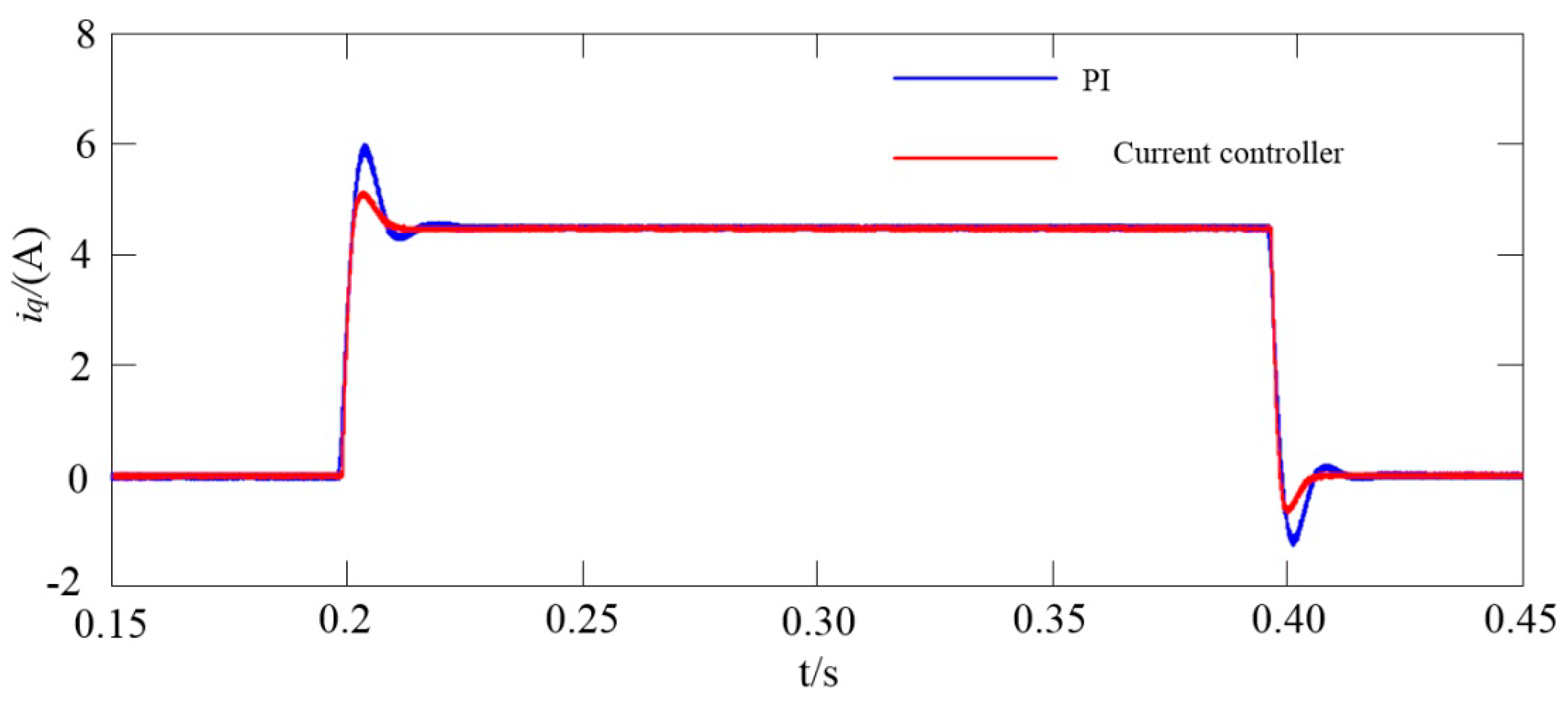
Load simulation, at 1000 r/min, 2 N·m at 0.2 s, and 2 N·m at 0.4 s, the current loop q–axis current response waveform controlled by the current controller and the PI is shown in Figure 10. In the dynamic process of load disturbance, the current overshoot of the current controller is significantly smaller than that of the PI controller, and it can enter a stable operation state in a short time in the face of load changes.

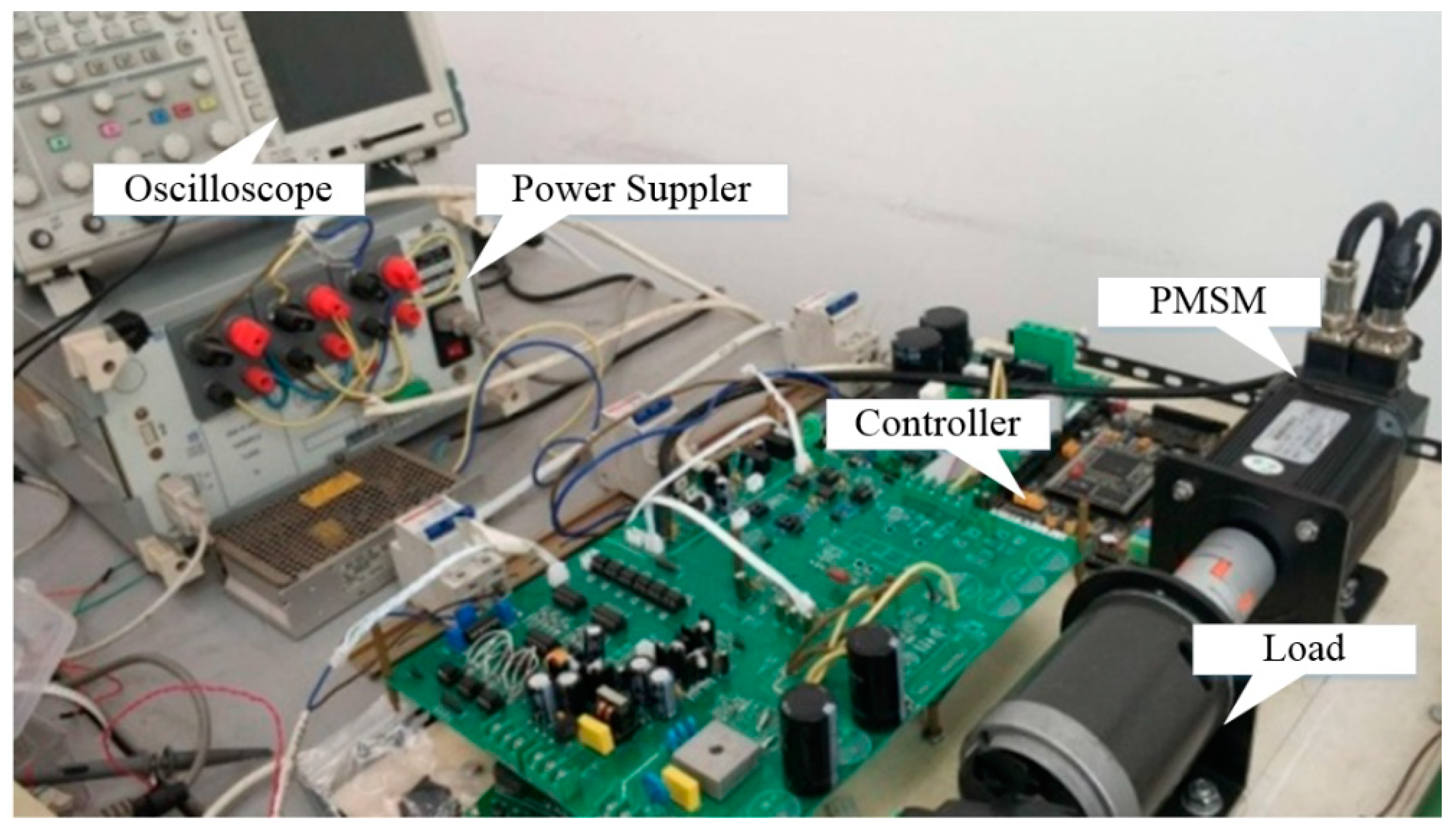
6. Experimental Verification

The system experiment platform is mainly composed of the PMSM motor, motor controller and host computer. The experimental platform can complete the collection of important information such as torque, rotation, voltage and current curve and power of the motor. The experimental platform of the motor drive control system is shown in Figure 11.

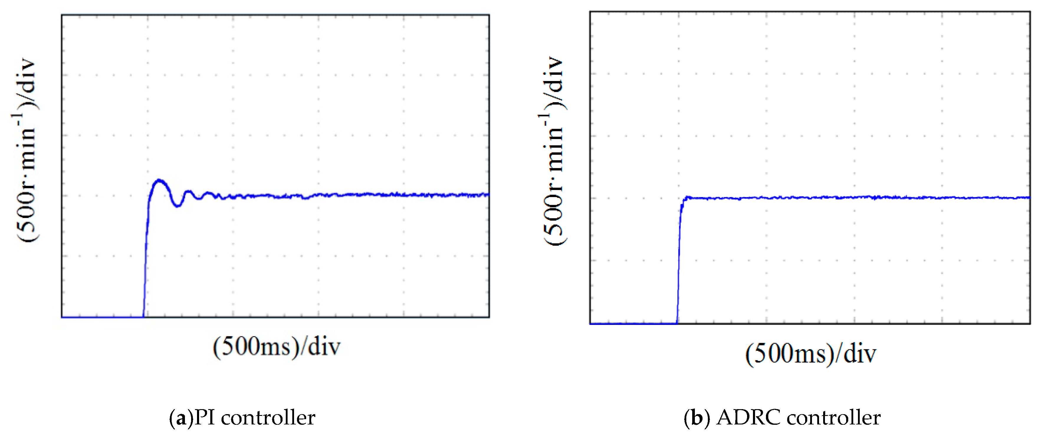
In order to verify that the control system has no overshooting response, the motor is unloaded and started at 1000 r/min. The results are shown in Figure 12, which reveals that under the same conditions the ADRC control quickly reaches the desired speed without causing the system overshoot. The overshoot of the PI controller is more obvious, and it will stabilize in 300 ms.

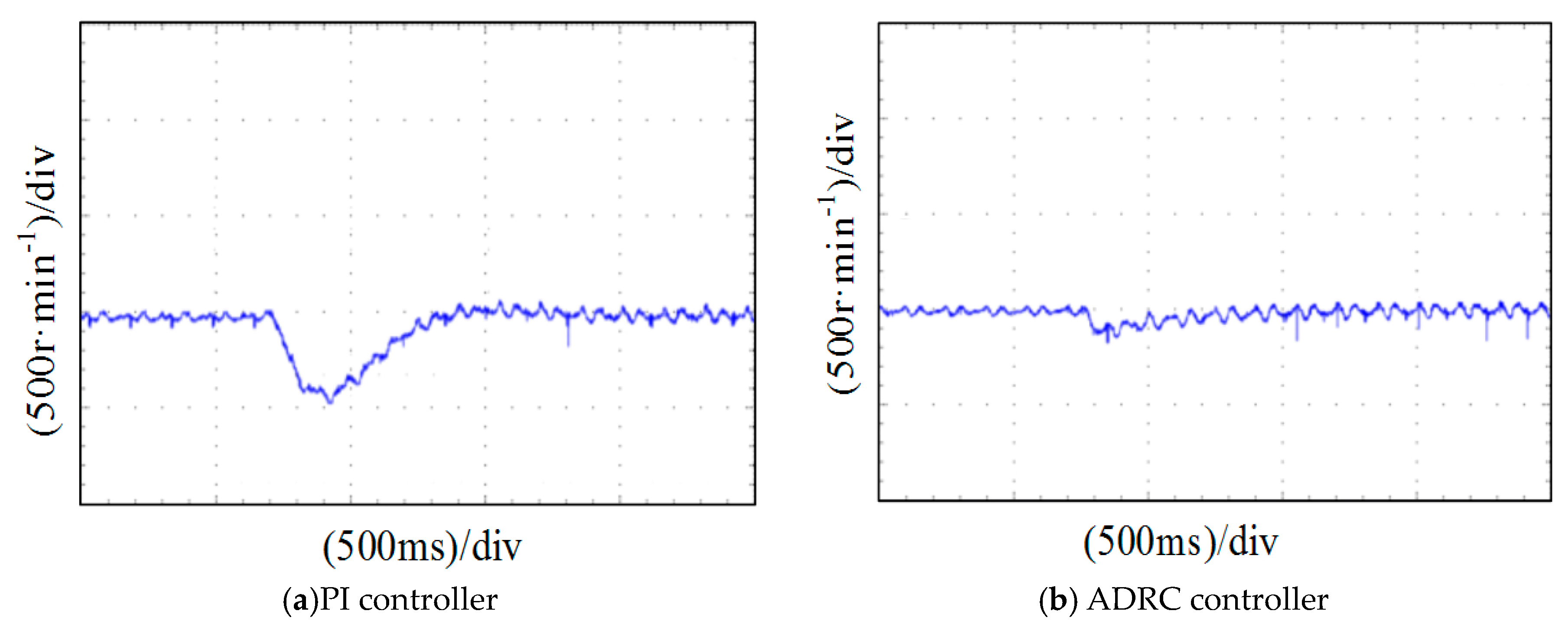
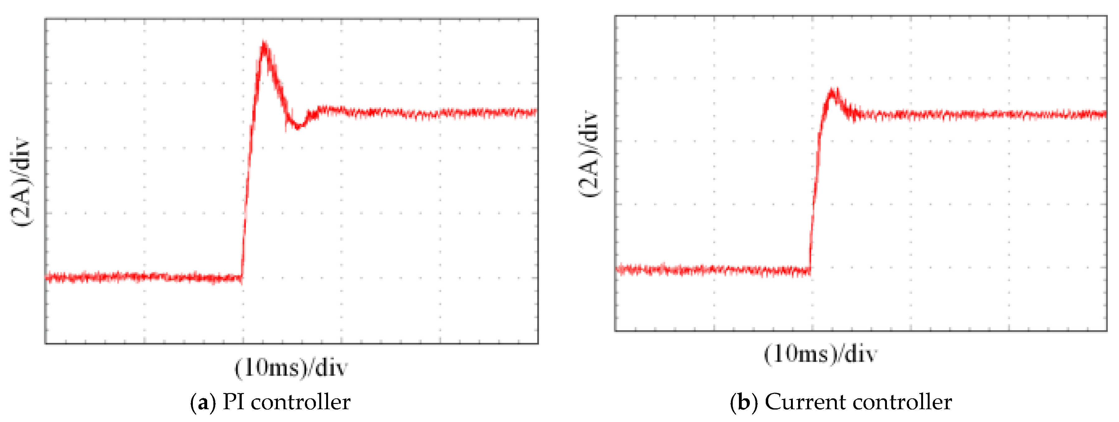
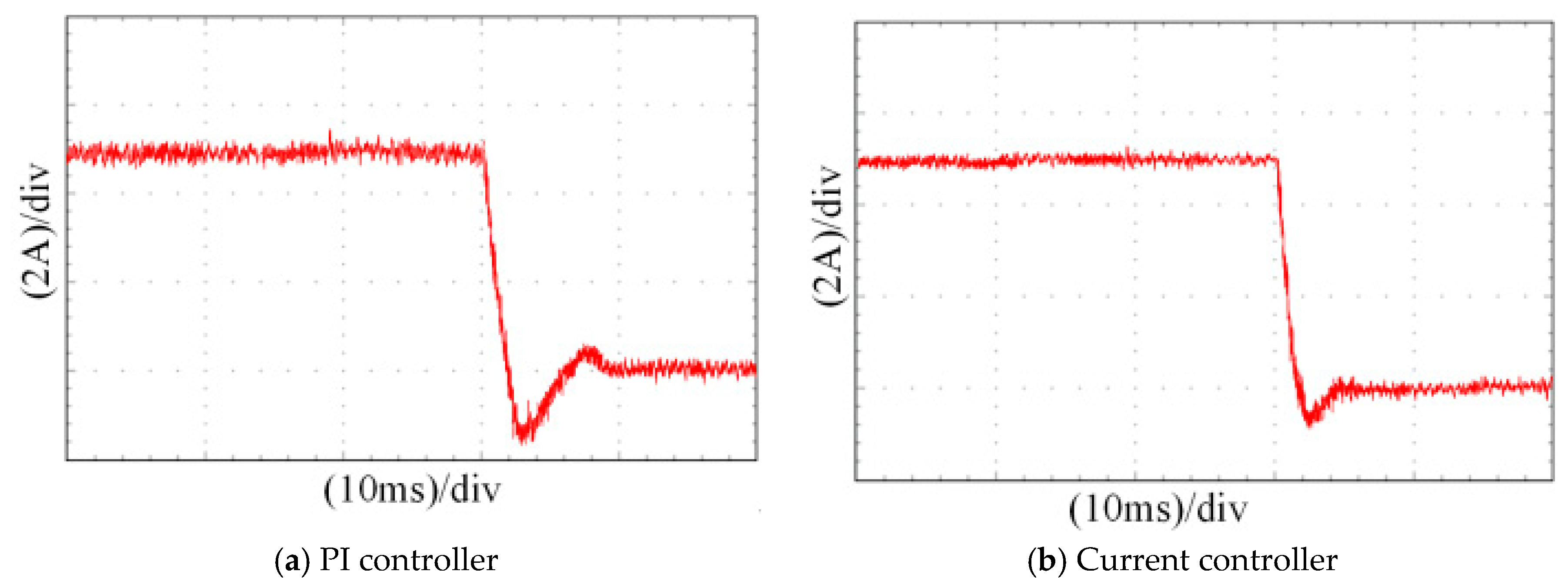
In order to verify the accuracy of our load changes, the initial load torque was zero, and became 2 N·m at 700 ms. Then uninstall to 0 N·m. The image of the PMSM speed is shown in Figure 13 and Figure 14. Comparing the these figures, it can be observed that under the ADRC controller that the speed of the system recovered more quickly following a disturbance, and the speed suffered less of a drop-off. The PI controller takes about 600 ms to recover, and the ADRC can be recovered in less than 300 ms. The experimental results are basically consistent with the simulation results. The current response curves of the q–axis during loading and unloading are shown in Figure 15 and Figure 16. The current overshoot of the q–axis is smaller and the recovery time is faster. When loading, the PI controller takes about 8 ms to stabilize, and the current controller only needs about 4 ms to stabilize. The peak voltage of the PI controller is 1.5 A larger than the current controller. The overall result is generally consistent with the simulation. Therefore, the ADRC has a more desirable control effect on the PMSM.

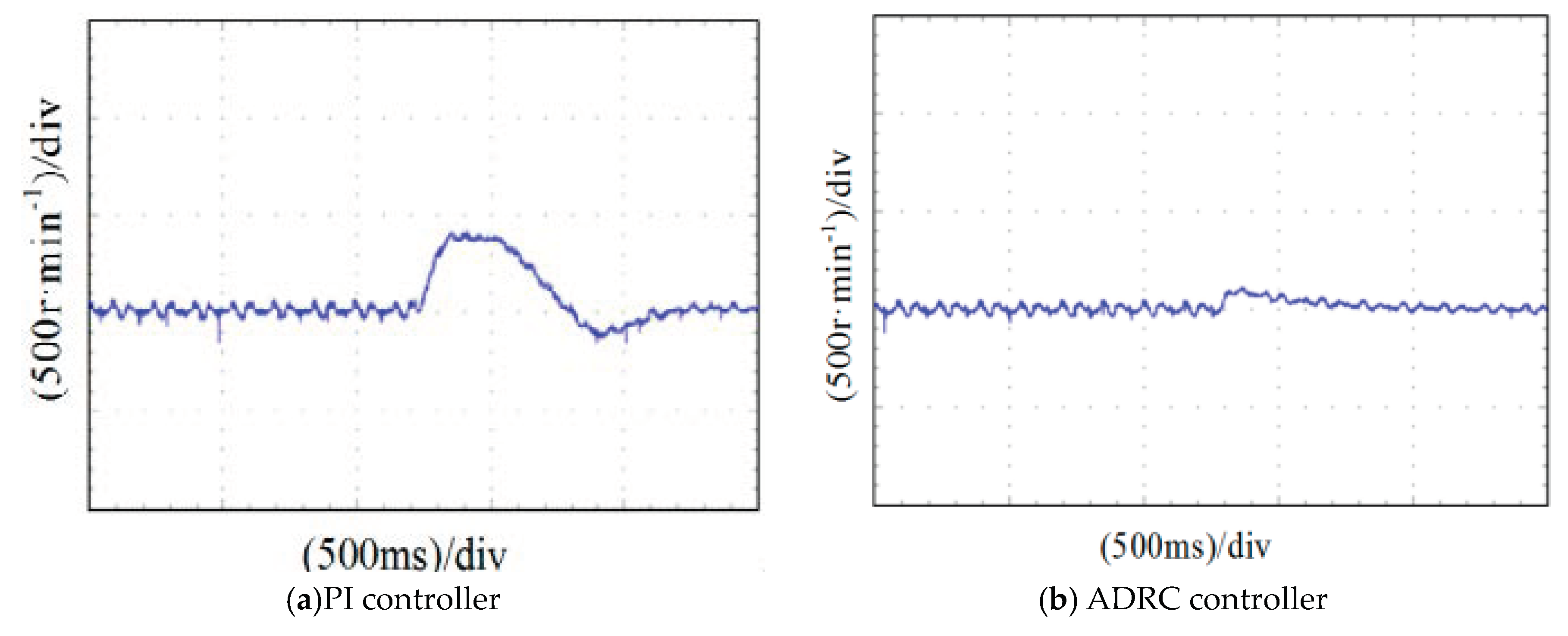
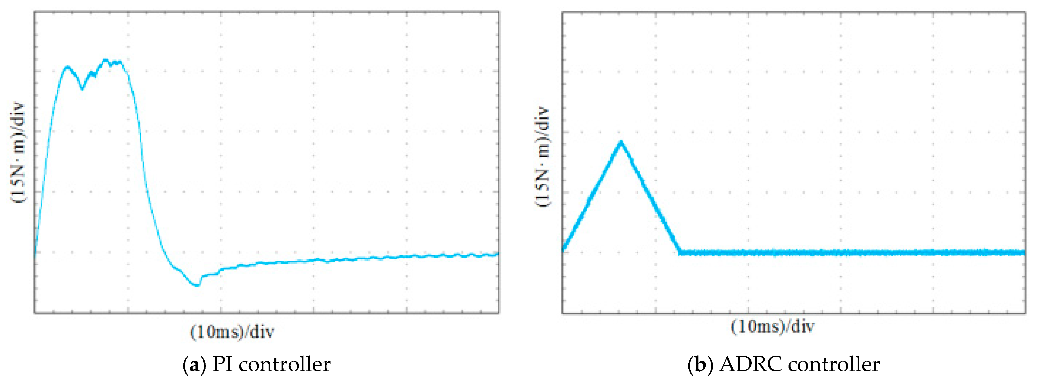
The motor starting torque under the two control methods is shown in Figure 17. When the ADRC control strategy is used, the torque waveform is a triangular wave, which is different from the phenomenon that the PI controller is saturated. This is the result of the TD affecting the transition process.

7. Conclusions

This paper proposes an active disturbances rejection control technology as the PMSM speed loop controller. It does not fully depend on the controlled object model. The variation of moment of inertia, stator resistance and other unknown disturbances are measured and compensated for by the ADRC speed loop, making the system strong against system parameter changes and external disturbances.

In order to achieve decoupling the complex coupling term of the PMSM, the feedback linearization algorithm is used to optimize the controller, and the decoupling control of the system is realized. The simulation and experimental research on the control system show that the control strategy has strong robustness, and the dynamic tracking performance is stable and accurate.