Countrywide Mobile Spectrum Sharing with Small Indoor Cells for Massive Spectral and Energy Efficiencies in 5G and Beyond Mobile Networks †


Abstract
1. Introduction
1.1. Background
1.2. Existing Literature
1.3. Contribution
1.4. Organization
1.5. Declaration
2. System Model
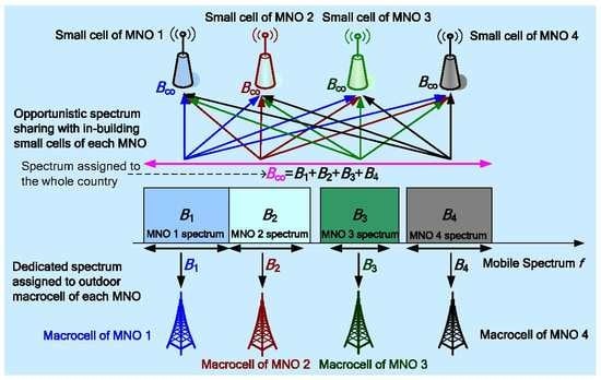
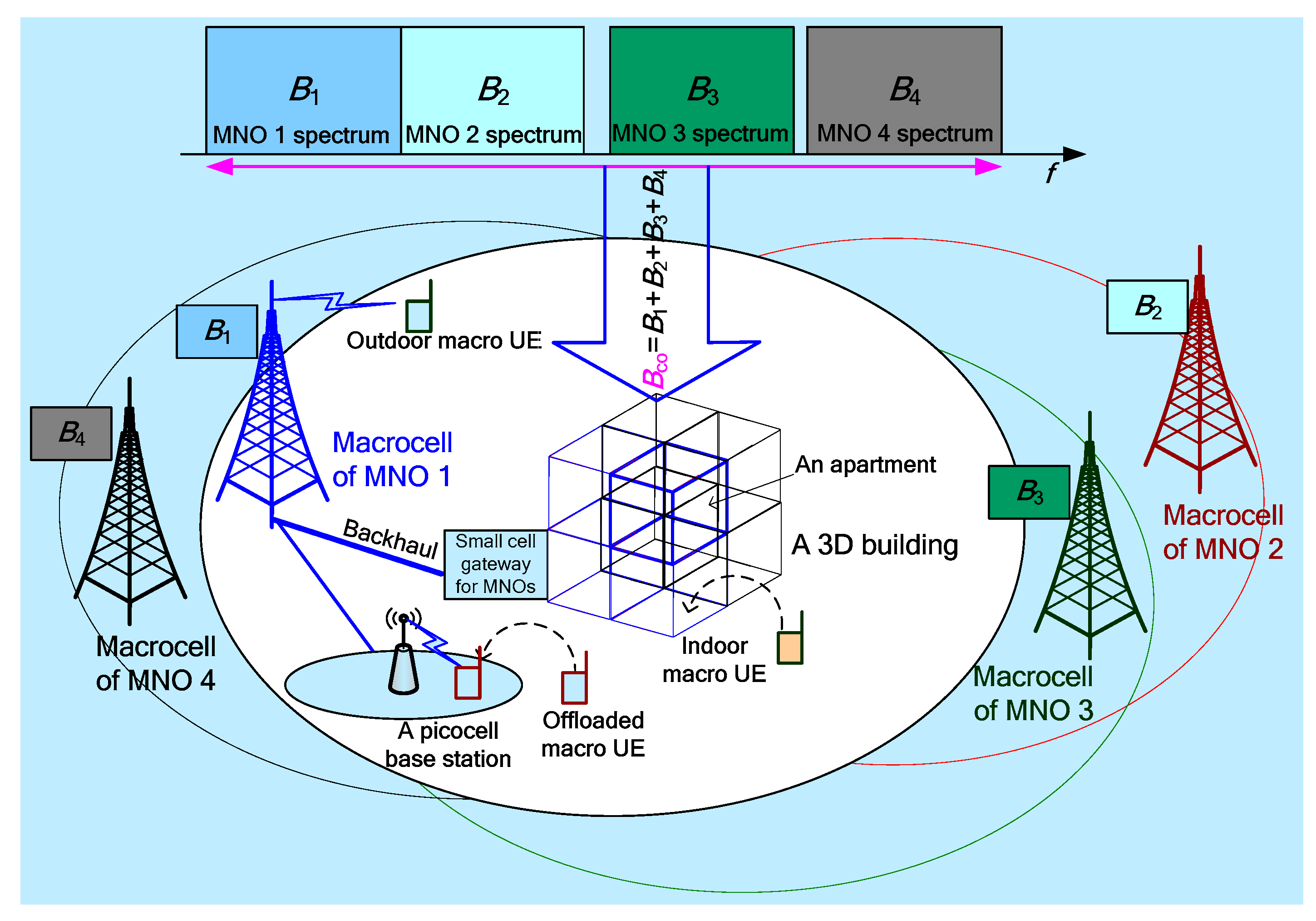
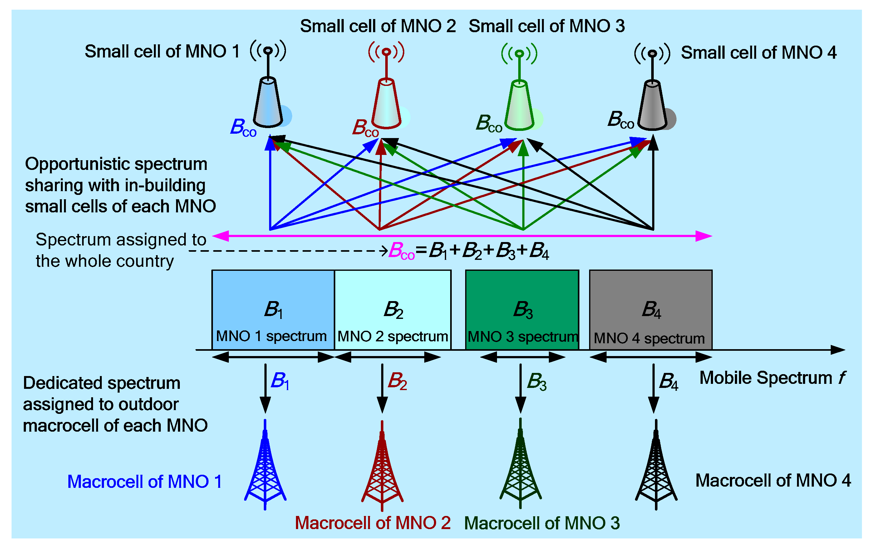
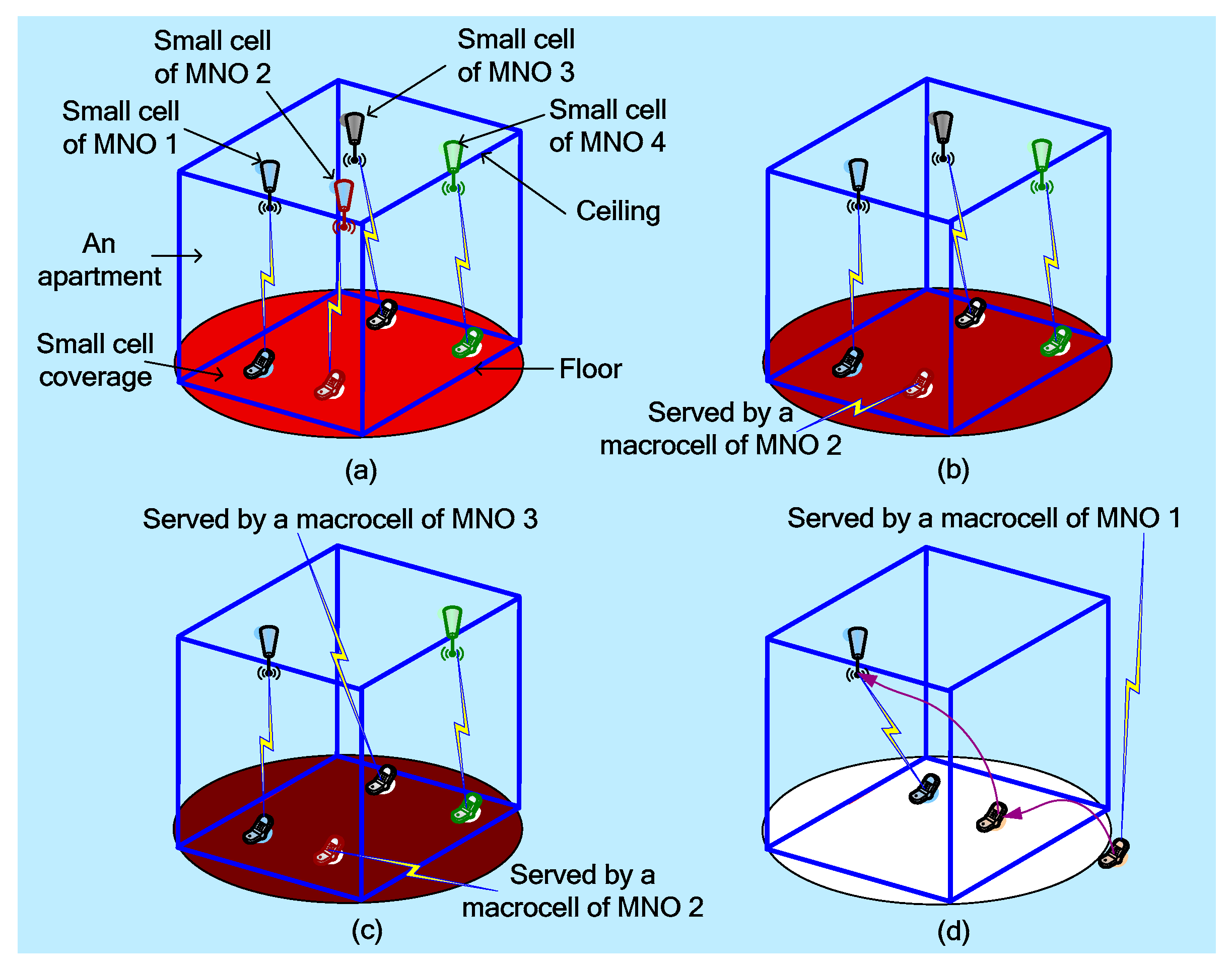
2.1. System Architecture
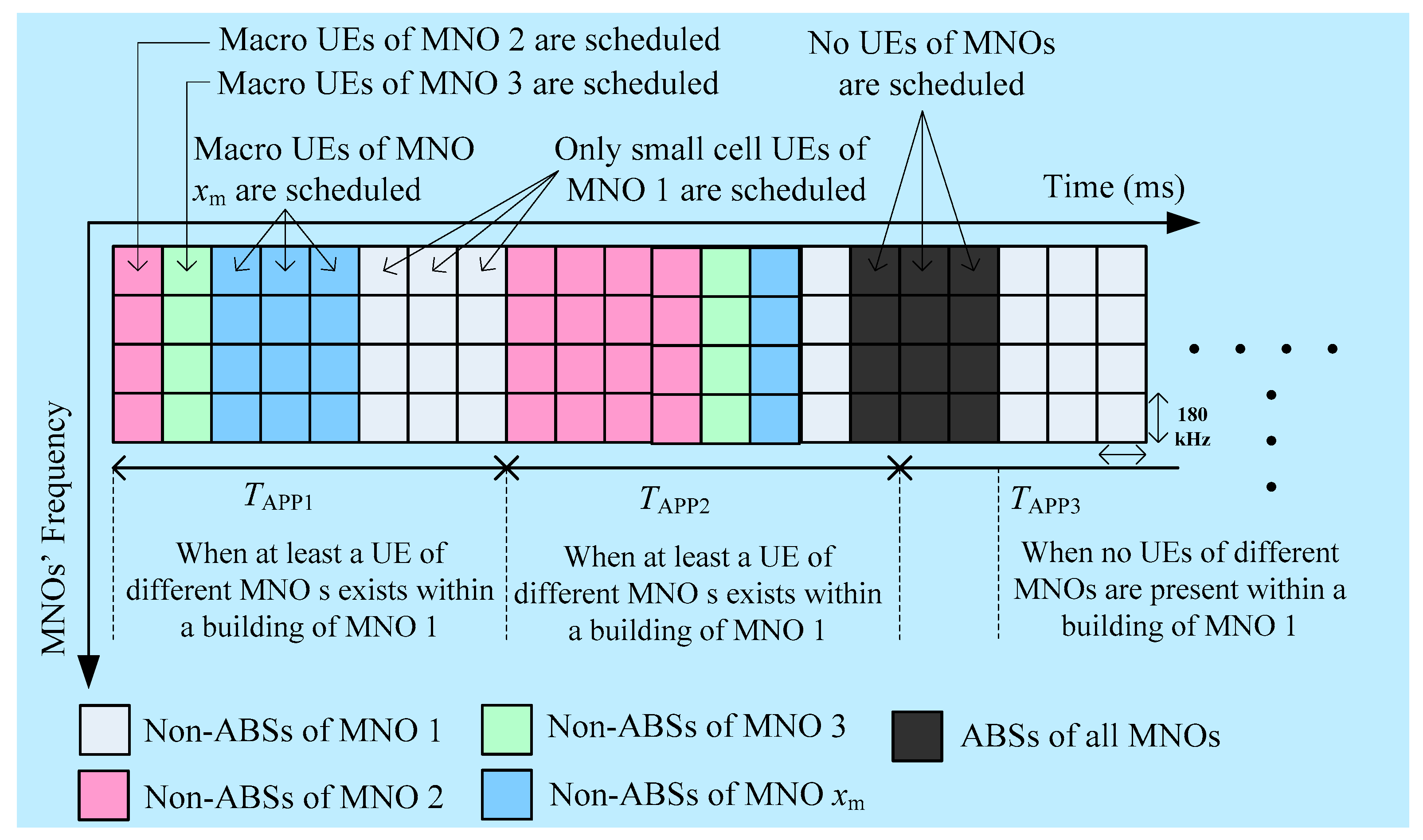
2.2. Proposed Spectrum sharing Technique and Related Issues
- (1)
- Issue 1: How to address dynamic resource allocation among MNOs to improve the overall spectrum utilization?How to address: The static allocation of the time resource based on the number of MNOs may cause either underutilization or scarcity of the spectrum of an MNO. To address this issue, we consider allocating the time resource to small cells of an MNO dynamically based on the actual traffic arrival rate in order to improve the spectrum utilization.
- (2)
- Issue 2: How to optimize for the fair allocation of the time resource to each MNO when applying the proposed nationwide spectrum sharing technique?How to address: We consider assigning an optimal number of transmission time intervals (TTIs) to an MNO x in proportion with the ratio of the average number of UEs of the MNO x to the sum of the average number of UEs of all other MNOs that are active during any APP.
- (3)
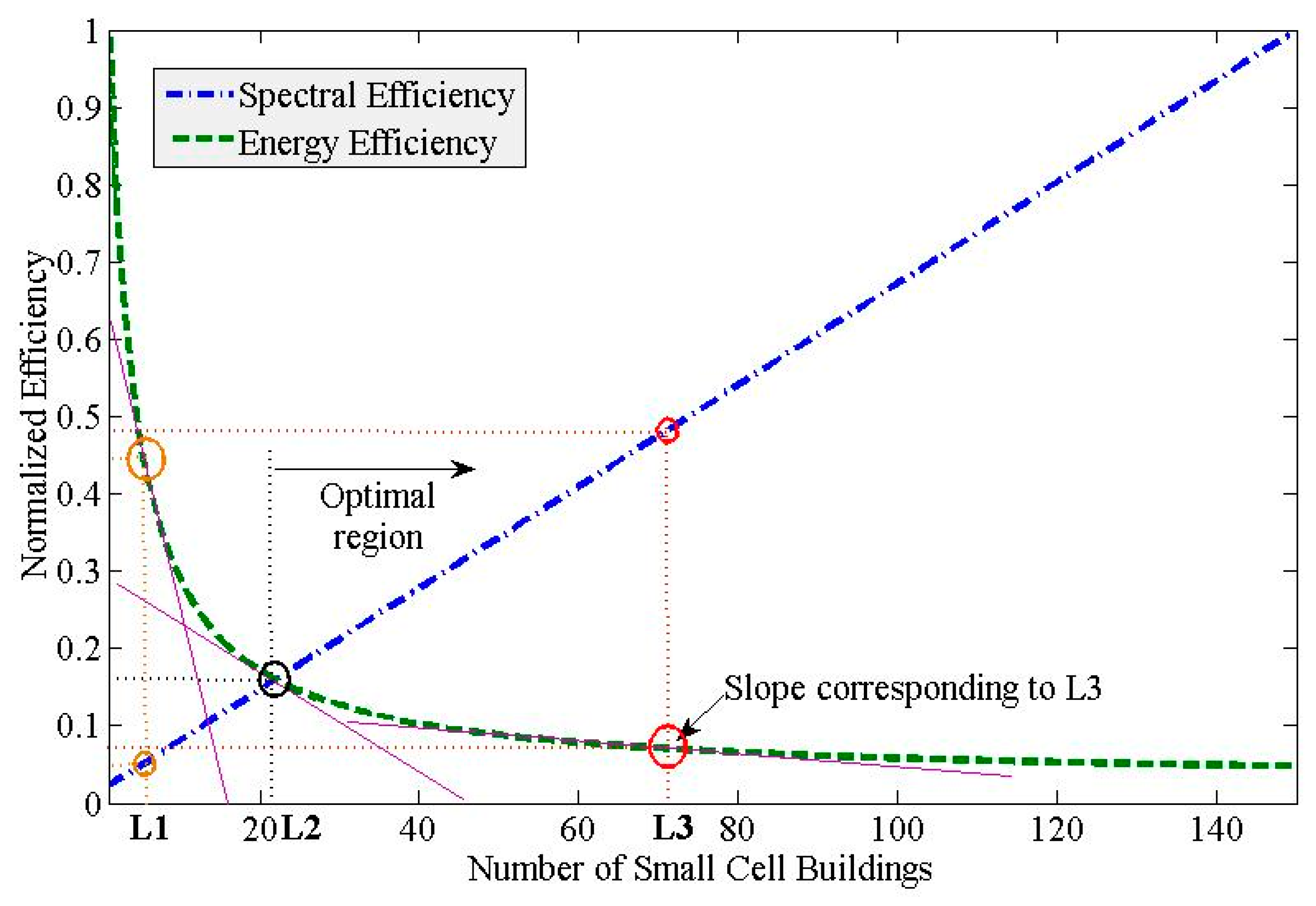
- Issue 3: How to ensure optimality between the spectral efficiency and the energy efficiency performances of an MNO for the proposed technique?How to address: we consider defining the minimum value of L denoted as Lmin by using the slope of the energy efficiency curve such that choosing any value of L ≥ Lmin results in improving both the spectral efficiency and energy efficiency responses of an MNO. The values of spectral and energy efficiencies corresponding to L ≥ Lmin define the region of optimality for both efficiencies. In other words, depending on the requirements for the spectral and energy efficiencies, an optimal value of L ≥ Lmin is chosen.
- (4)
- Issue 4: How to clarify that the proposed technique is scalable and can meet the spectral and energy efficiencies of the next-generation mobile networks?How to Address: To ensure scalability, we consider sharing the whole spectrum with small cells per building L per MNO such that by increasing the value of L subject to L ≥ Lmin more spectral efficiency and energy efficiency could be achieved. Further, in the paper, we show that by adjusting the value of L corresponding to the varying number of TTIs allocated to an MNO during each APP, the spectral efficiency and the energy efficiency requirements for the 5G mobile network could be achieved.
- (5)
- Issue 5: How to describe and address the CCI scenarios in the proposed technique. Also, how does the CCI affect the point of optimality for spectral and energy efficiencies?How to address: We describe in detail the CCI due to the presence of multiple MNOs operating at the spectrum using the ABS based enhanced intercell interference coordination (eICIC) technique. Since with the change of CCI, the number of TTIs allocated to an MNO change, an optimal number of TTIs is allocated to each MNO based on the actual traffic demand of the MNO as compared to that of the others. In general, since an increase in CCI results in degrading the spectral and efficiency performances, the minimum point of optimality in terms of L, corresponding to which both the spectral and energy efficiencies intersect one another, shifts leftward resulting in a decrease in the minimum optimal point Lmin and vice versa.
3. Co-Channel Interference Scenario and Management
3.1. Co-Channel Interference Scenario
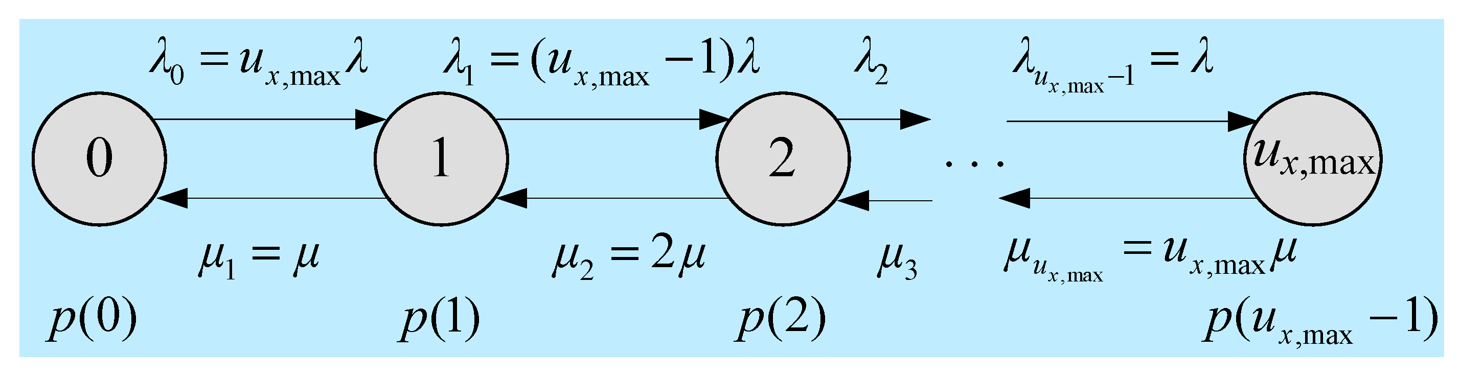
3.2. Defining Call Arrivals of Small Cells per MNO
3.3. Co-Channel Interference Management
4. Performance Metrics Estimation
4.1. Capacity, Spectral Efficiency, and Energy Efficiency Performance
4.2. System-Level Performance Analysis
5. Modeling Energy Efficiency and the Condition for Optimality
5.1. Modeling Energy Efficiency
5.2. Condition for Optimality
6. Proposed Algorithm and Default Parameters and Assumptions
| Algorithm 1 Proposed spectrum sharing technique among all MNOs of a country |
 |
7. Performance Analysis and Comparison
7.1. Impact of on
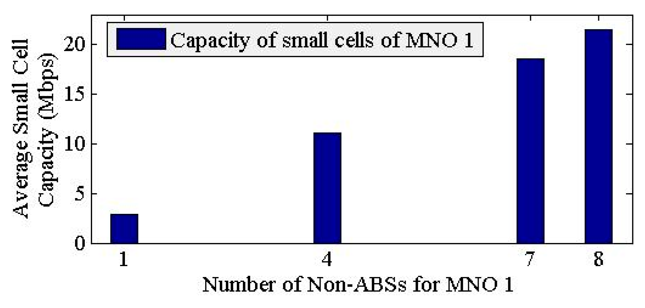
7.2. Impact of on Capacity, Spectral Efficiency, and Energy Efficiency
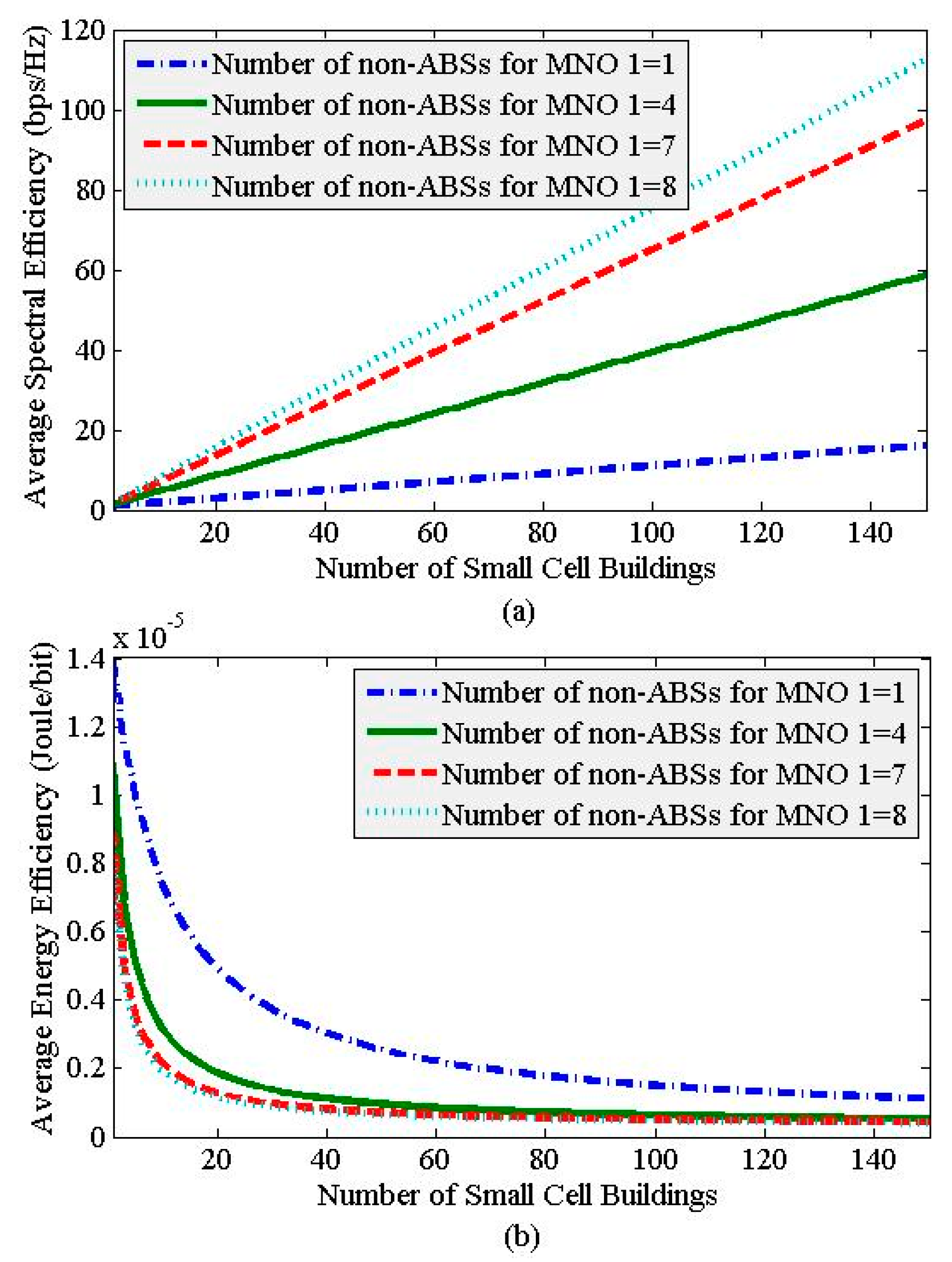
7.3. Spectral Efficiency and Energy Efficiency Performances
7.4. Performance Comparison with 5G Requirements
8. Conclusions
Funding
Acknowledgments
Conflicts of Interest
References
- Saquib, N.; Hossain, E.; Kim, D.I. Fractional frequency reuse for interference management in LTE-advanced hetnets. IEEE Wirel. Commun. 2013, 20, 113–122. [Google Scholar] [CrossRef]
- Guidotti, A.; Vanelli-Coralli, A.; Conti, M.; Andrenacci, S.; Chatzinotas, S.; Maturo, N.; Evans, B.; Awoseyila, A.; Ugolini, A.; Foggi, T.; et al. Architectures and key technical challenges for 5G systems incorporating satellites. IEEE Trans. Veh. Technol. 2019, 68, 2624–2639. [Google Scholar] [CrossRef]
- Saha, R.K. Spectrum Sharing in Satellite-Mobile Multisystem Using 3D In-Building Small Cells for High Spectral and Energy Efficiencies in 5G and Beyond Era. IEEE Access 2019, 7, 43846–43868. [Google Scholar] [CrossRef]
- Saha, R.K. Realization of Licensed/Unlicensed Spectrum Sharing Using eICIC in Indoor Small Cells for High Spectral and Energy Efficiencies of 5G Networks. Energies 2019, 12, 2828. [Google Scholar] [CrossRef]
- Kamal, H.; Coupechoux, M.; Godlewski, P. Inter-operator spectrum sharing for cellular networks using game theory. In Proceedings of the 2009 IEEE 20th International Symposium on Personal, Indoor and Mobile Radio Communications, Tokyo, Japan, 13–16 September 2009; pp. 425–429. [Google Scholar]
- Bennis, M.; Debbah, M.; Lasaulce, S. Inter-Operator Spectrum Sharing from a Game Theoretical Perspective. EURASIP J. Adv. Signal Process. 2009, 2009, 295739. [Google Scholar] [CrossRef][Green Version]
- Jorswieck, E.A.; Badia, L.; Fahldieck, T.; Karipidis, E.; Luo, J. Spectrum sharing improves the network efficiency for cellular operators. IEEE Commun. Mag. 2014, 52, 129–136. [Google Scholar] [CrossRef]
- Joshi, S.K.; Manosha, K.B.S.; Codreanu, M.; Latva-aho, M. Dynamic inter-operator spectrum sharing via Lyapunov optimization. IEEE Trans. Wirel. Commun. 2017, 16, 6365–6381. [Google Scholar] [CrossRef]
- Tehrani, R.H.; Vahid, S.; Triantafyllopoulou, D.; Lee, H.; Moessner, K. Licensed Spectrum Sharing Schemes for Mobile Operators: A Survey and Outlook. IEEE Commun. Surv. Tutor. 2016, 18, 2591–2623. [Google Scholar] [CrossRef]
- The Electronic Communications Committee. “Licensed shared access (LSA),” ECC Report 205, The Electronic Communications Committee, Copenhagen, Denmark, 2014. Available online: https://www.ecodocdb.dk/download/baa4087d-e404/ECCREP205.PDF (accessed on 30 June 2019).
- Asp, A.; Sydorov, Y.; Keskikastari, M.; Valkama, M.; Niemela, J. Impact of Modern Construction Materials on Radio Signal Propagation: Practical Measurements and Network Planning Aspects. In Proceedings of the 2014 IEEE 79th Vehicular Technology Conference (VTC Spring), Seoul, Korea, 18–21 May 2014; pp. 1–7. [Google Scholar]
- Saha, R.K. Nationwide spectrum sharing of mobile network operators with indoor small cells. In Proceedings of the IEEE International Symposium on Dynamic Spectrum Access Networks (IEEE DySPAN), Newark, NJ, USA, 11–14 November 2019. [Google Scholar]
- Chimeh, J.D.; Hakkak, M.; Alavian, S.A. Internet Traffic and Capacity Evaluation in UMTS Downlink. In Proceedings of the Future Generation Communication and Networking (FGCN 2007), Jeju, Korea, 6–8 December 2007; pp. 547–552. [Google Scholar]
- European Telecommunications Standards Institute (ETSI); Universal Mobile Telecommunications System (UMTS). Selection Procedures for the Choice of Radio Transmission Technologies of the UMTS. European Telecommunications Standards Institute (ETSI); Sophia Antipolis Valbonne, France, TR 101 112, UMTS 30.03, ver. 3.2.0, 1998–2004. Available online: https://www.etsi.org/deliver/etsi_tr/101100_101199/101112/03.02.00_60/tr_101112v030200p.pdf (accessed on 2 January 2017).
- Kleinrock, L. Queueing Systems, Vol I: Theory; Wiley-Interscience: New York, NY, USA, 1975. [Google Scholar]
- Pérez-Romero, J.; Sallent, O.; Agustí, R.; Díaz-Guerra, M.A. Radio Resource Management Strategies in UMTS; Wiley: Hoboken, NJ, USA, 2005. [Google Scholar]
- Saha, R.K. Multiband spectrum sharing with indoor small cells in Hybrid Satellite-Mobile systems. In Proceedings of the 2019 IEEE 90th Veh. Tech. Conf. (VTC2019-Fall), Honolulu, HI, USA, 22–25 September 2019; pp. 1–7. [Google Scholar]
- Saha, R.K. A technique for massive spectrum sharing with ultra-dense in-building small cells in 5G era. In Proceedings of the 2019 IEEE 90th Veh. Tech. Conf. (VTC2019-Fall), Honolulu, HI, USA, 22–25 September 2019; pp. 1–7. [Google Scholar]
- Ellenbeck, J.; Schmidt, J.; Korger, U.; Hartmann, C. A Concept for Efficient System-Level Simulations of OFDMA Systems with Proportional Fair Fast Scheduling. In Proceedings of the 2009 IEEE Globecom Workshops, Honolulu, HI, USA, 30 November–4 December 2009; pp. 1–6. [Google Scholar]
- E-UTRA. Radio Frequency (RF) System Scenarios; Document 3GPP TR 36.942; 3rd Generation Partnership Project: Sophia Antipolis Valbonne, France, 2007. [Google Scholar]
- Simulation Assumptions and Parameters for FDD HeNB RF Requirements; Document TSG RAN WG4R4-092042; Alcatel-Lucent, picoChip Designs, Vodafone: San Francisco, CA, USA, 2009.
- Geng, S.; Kivinen, J.; Zhao, X.; Vainikainen, P. Millimeter-wave propagation channel characterization for short-range wireless communications. IEEE Trans. Veh. Technol. 2009, 58, 3–13. [Google Scholar] [CrossRef]
- Saha, R.K.; Saengudomlert, P.; Aswakul, C. Evolution toward 5G mobile networks-A survey on enabling technologies. Eng. J. 2016, 20, 87–119. [Google Scholar] [CrossRef]
- Wang, C.-X.; Haider, F.; Gao, X.; You, X.-H.; Yang, Y.; Yuan, D.; Aggoune, H.; Haas, H.; Fletcher, S.; Hepsaydir, E. Cellular architecture and key technologies for 5G wireless communication networks. IEEE Commun. Mag. 2014, 52, 122–130. [Google Scholar] [CrossRef]
- Auer, G.; Giannini, V.; Gódor, I.; Blume, O.; Fehske, A.; Rubio, J.A.; Frenger, P.; Olsson, M.; Sabella, D.; Gonzalez, M.J.; et al. How much energy is needed to run a wireless network? In Green Radio Communication Networks; Cambridge University Press (CUP): Cambridge, UK, 2012; pp. 359–384. [Google Scholar]


| Parameters and Assumptions | Value | |||
|---|---|---|---|---|
| E-UTRA simulation case 1 | 3GPP case 3 | |||
| Cellular layout 2 and Inter-site distance (ISD) 1,2 | Hexagonal grid, dense urban, 3 sectors per macrocell site and 1732 m | |||
| Carrier frequency 2,3 and transmit direction | 2 GHz and downlink | |||
| Number of MNOs xm | 4 | |||
| Bandwidth per MNO Bop | 1 MHz | |||
| Considered MNO for performance evaluation | MNO 1 | |||
| Number of cells of MNO1 | 1 macrocell, 2 picocells, 8 SBSs per building | |||
| Total base station transmit power 1 (dBm) of MNO 1 | 46 for microcell 1,4, 37 for picocell 1, 20 for SBS 1,3,4 | |||
| Co-channel fading model 1 | Frequency selective Rayleigh for the macrocell and picocells, and Rician for SBSs | |||
| External wall penetration loss 1 (Low) of a building | 20 dB | |||
| Path loss for MNO 1 | Macocell BS (MBS) and a UE 1 | Indoor macro UE | PL (dB) = 15.3 + 37.6 log10R, R is in m | |
| Outdoor macro UE | PL (dB) = 15.3 + 37.6 log10R + Low, R is in m | |||
| Picocell BS (PBS) and a UE 1 | PL (dB) = 140.7 + 36.7log10R, R is in km | |||
| SBS and a UE 1,2,3 | PL (dB) = 127 + 30 log10 (R/1000), R is in m | |||
| Lognormal shadowing standard deviation (dB) | 8 for MBS 2, 10 for PBS 1, and 10 for SBS 2,3 | |||
| Antenna configuration | Single-input single-output for all base stations and UEs | |||
| Antenna pattern (horizontal) | Directional (120°) for microcell 1, omnidirectional for picocell 1 and SBS 1 | |||
| Antenna gain plus connector loss (dBi) | 14 for MBS 2, 5 for PBS 1, 5 for SBS 1,3 | |||
| UE antenna gain 2,3 | 0 dBi | |||
| UE noise figure 2 and UE speed 1 | 9 dB, 3 km/h | |||
| Total number of macro UEs | 30 | |||
| Maximum number of small cell UEs served simultaneously by an SBS | 1 | |||
| Picocell coverage and macro UEs offloaded to all picocells 1 | 40 m (radius), 2/15 | |||
| 3D multistory building and SBS models (regular square-grid) for MNO 1 | Number of buildings | L | ||
| Number of floors per building | 2 | |||
| Number of apartments per floor | 4 | |||
| Number of SBSs per apartment | 1 | |||
| SBS activation ratio | 100% | |||
| SBS deployment ratio | 1 | |||
| Total number of SBSs per building | 8 | |||
| Area of an apartment | ||||
| Location of an SBS in an apartment | center | |||
| Scheduler and traffic model 2 | Proportional Fair (PF) and full buffer | |||
| Type of SBSs | Closed Subscriber Group femtocell base stations | |||
| Channel State Information (CSI) | Ideal | |||
| TTI 1, scheduler time constant (tc), TAPP | 1 ms, 100 ms, 8 ms | |||
| Maximum simulation run time | (8 × TAPP) ms | |||
| TnABSs,1 | Lmin (To Meet Requirements for 5G Mobile Networks) | ||
|---|---|---|---|
| Spectral Efficiency (bps/Hz/cell) | |||
| 1 | 356 | 41 | 356 |
| 4 | 94 | 11 | 94 |
| 7 | 57 | 7 | 57 |
| 8 | 49 | 6 | 49 |
© 2019 by the author. Licensee MDPI, Basel, Switzerland. This article is an open access article distributed under the terms and conditions of the Creative Commons Attribution (CC BY) license (http://creativecommons.org/licenses/by/4.0/).
Share and Cite
Saha, R.K. Countrywide Mobile Spectrum Sharing with Small Indoor Cells for Massive Spectral and Energy Efficiencies in 5G and Beyond Mobile Networks. Energies 2019, 12, 3825. https://doi.org/10.3390/en12203825
Saha RK. Countrywide Mobile Spectrum Sharing with Small Indoor Cells for Massive Spectral and Energy Efficiencies in 5G and Beyond Mobile Networks. Energies. 2019; 12(20):3825. https://doi.org/10.3390/en12203825
Chicago/Turabian StyleSaha, Rony Kumer. 2019. "Countrywide Mobile Spectrum Sharing with Small Indoor Cells for Massive Spectral and Energy Efficiencies in 5G and Beyond Mobile Networks" Energies 12, no. 20: 3825. https://doi.org/10.3390/en12203825
APA StyleSaha, R. K. (2019). Countrywide Mobile Spectrum Sharing with Small Indoor Cells for Massive Spectral and Energy Efficiencies in 5G and Beyond Mobile Networks. Energies, 12(20), 3825. https://doi.org/10.3390/en12203825