Article

A Weekend Load Forecasting Model Based on Semi-Parametric Regression Analysis Considering Weather and Load Interaction

Guangxi Key Laboratory of Power System Optimization and Energy Technology, Guangxi University, Nanning 530004, China
*
Author to whom correspondence should be addressed.
Energies 2019, 12(20), 3820; https://doi.org/10.3390/en12203820
Submission received: 19 September 2019 / Revised: 1 October 2019 / Accepted: 2 October 2019 / Published: 10 October 2019
(This article belongs to the Section F: Electrical Engineering)

Abstract

:
Compared to the load characteristics of normal working days, weekend load characteristics have a low level of load and are sensitive to meteorological conditions, which influences the accuracy of short-term weekend-load forecasting. To solve this problem and to improve the accuracy of short-term weekend-load forecasting, a Semi-parametric weekend-load forecasting method based on the interaction between meteorological and load is proposed in this paper. The main work is shown as follows: (1) through separating weekend-load from normal-load and analyzing the correlation between meteorological factors and daily maximum load, the meteorological factors with parameter characteristics and non-parameter characteristics can be screened out; (2) a short-term weekend-load forecasting model is built according to Semi-parametric regression theory which can express the coupling relation between meteorology and load more realistically; (3) the effect of temperature accumulation is also considered to correct the forecasting model. The proposed method is proved by implementing short-term weekend-load forecasting on the real historical data of the Southern Power Grid in China. The result shows that the 96-point mean load forecasting accuracy obtained by this model can meet the requirement of power network operation.

1. Introduction

With the expansion of the power grid scale and the increasing of load peak and valley differences, it has become an important and arduous task for power dispatching departments to improve the accuracy of short-term load forecasting. The accuracy of forecasting results not only affects the competition mechanism of the power market but also plays an important role in the safe and stable operation of the power system.
Compared to the load characteristics of normal working days, the weekend load has a low level of load and is sensitive to meteorological conditions. With a strong coupling relationship between meteorology and load, the impact of meteorology on load is multi-layered, showing randomness and uncertainty. The randomness of meteorology is not just a simple linear function relation or a set of mathematical equations that can be expressed—it needs to comprehensively take the effect of external meteorology into account. It should not only consider the effect of the current temperature on load but should also pay attention to the variation of load lag temperature, that is, the temperature agglomeration effect [1,2], which also had a certain impact on weekend load. Therefore, the study of the coupling relationship between meteorology and load is the key to improve the accuracy of weekend load forecasting and all-weather short-term load forecasting.
For a long time, many experts have been focusing on research on short-term load forecasting. The forecasting methods such as the time series method [3,4], support vector machine method [5,6,7,8,9,10], random forest models [11,12,13,14], artificial neural network method [5,15,16,17,18,19,20] and grey theory [21,22,23] could be applied to general weekday scenes and obtain good results. However, the difference between characteristics on weekend load and working days, as well as the interactive coupling relationship with external weather information, have become the shortcoming factors that restrict the accuracy of weekend load forecasting. At the same time, the mainstream forecasting methods mostly belong to the category of parameter statistics, in which the dependent variable has a strong dependence on the input variable. In this case, when the set function model is valid, the accuracy of forecasting results is ideal; but when the function model is invalid, the fitting degree and forecasting accuracy of the model is not satisfactory. Therefore, it is not entirely applicable to weekend load forecasting with randomness and uncertainty. The Semi-parametric regression model contains two parts: parametric and non-parametric, which concentrates the information on a clear relation part but does not ignore the effect of interference factors (non-parameters part) [24]. Reference [25] suggests a Semi-parametric approach based on generalized additive models theory to model electrical load and the methodology has been applied with good results on the actual grid. In [26], based on the preliminary prediction model, the temperature accumulation effect correction is considered to reduce the local error of the load forecasting.
In this paper, the power system weekend load forecasting is considered as a whole of the mutual coupling of meteorology and load, and then the weekend load forecasting model for multi-source meteorological factors is established. When the load data is preprocessed, the load data is mainly divided into three types according to the date type of the load, such as normal working day, weekend and holiday, and each type of data has a corresponding date type. The samples modeled by filtering all have the same date type, and the influence of date type can be approximately ignored. The monthly standardized processing of historical load can weaken the influence of economic growth rate on load level. Therefore, the forecasting of the weekend load is ultimately to study the effect of external meteorological factors on the load, that is, the mutual coupling relationship between the two. The uncontrollability of the external meteorological conditions brings challenges to load forecasting. In this paper, by analyzing the correlation degree of each meteorological factor and load, the meteorological factors are divided into two categories: parametric and non-parametric. This method improves the accuracy of weekend load forecasting by optimizing the allocation of meteorological factors.
The rest of the paper is arranged as follows: the interaction of meteorology and load is analyzed in Section 2. The basic Semi-parametric regression model and its parameters estimation calculation process are introduced in detail in Section 3. The proposed forecasting of the weekend load based on Semi-parametric Regression model are described in Section 4. The explanation of temperature accumulation effect correction is given in Section 5. The forecasting of weekend load level, the forecasting of weekend load curve model, the forecasting and correction for 96-point weekend load curve and the judgment basis for forecasting results are presented in Section 6. The sample load forecasting based on semi-parametric method and the comparison and analysis of model prediction results are provided in Section 7. Finally, conclusions are given in Section 8.

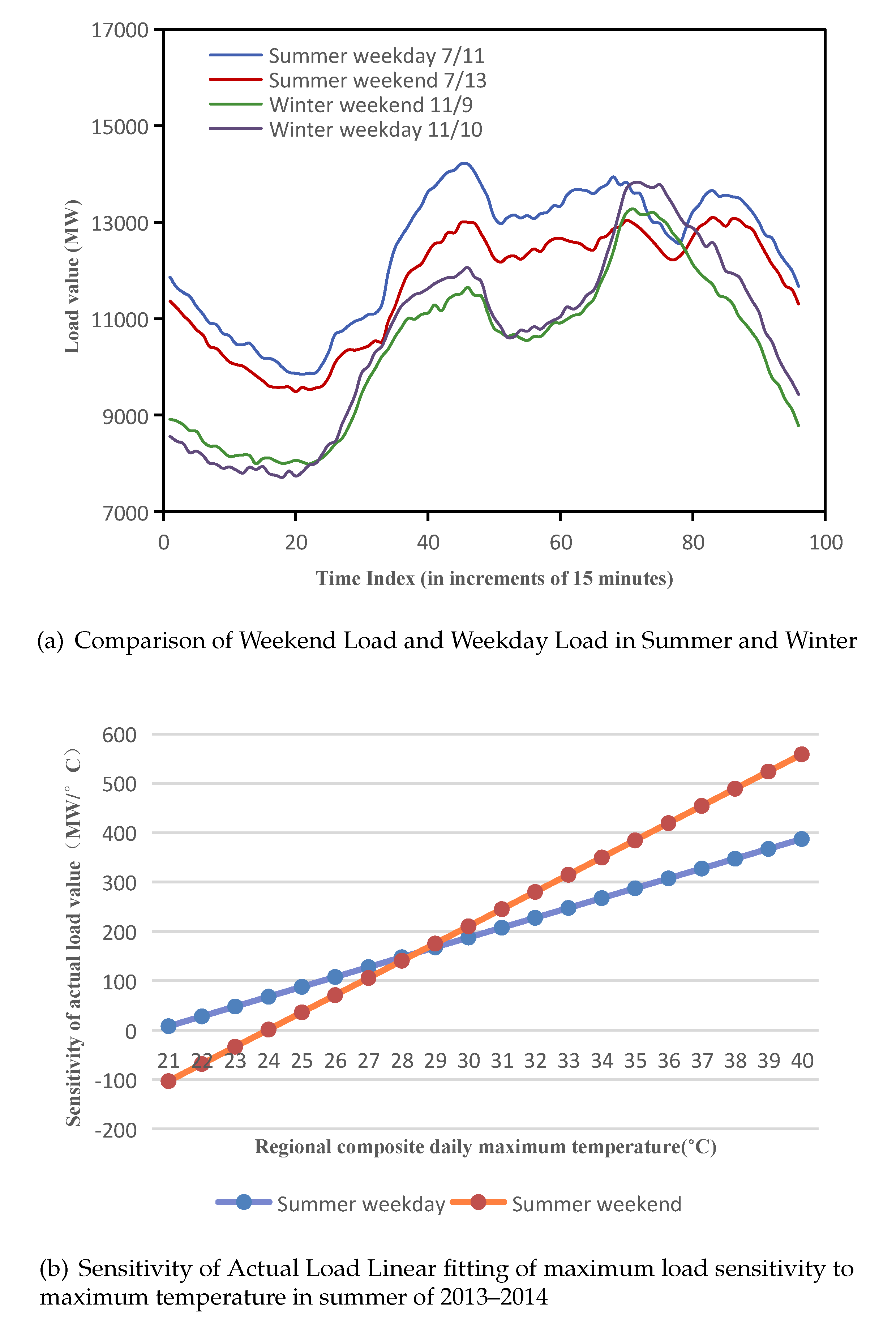
2. The Interaction of Meteorology and Load

The weekend load forecast is deeply influenced by various factors, including cultural activities, meteorology, economic growth rate and so on. With the continuous improvement of people’s pursuit of quality of life, people generally choose to rest or go out for activities on weekends; large user production load and enterprise load exit, resulting in a certain reduction in the load level compared with the working days. And commercial loads and other loads sensitive to meteorological changes increase in weight, making the weekend loads more deeply affected by meteorological factors. From Figure 1a, it can be seen that although the weekend load curve is similar to the general weekday load curve, the overall shape of the weekend load curve and the peak-valley difference of the load are different from those of the weekday. The early peak and the late peak of the load curve decrease in proportion to the working day. Evidently, the weekend load level is lower than that of the working day, and the shape of the load curve is different from that of the working day. This load characteristic is more obvious in summer weekend. In addition, taking summer as an example, by comparing the linear fitting of maximum load to maximum temperature sensitivity in summer of 2013–2014 as shown in Figure 1b, it can be found that the slope of sensitivity curve in summer weekend is larger than that for a summer weekday, which means that the maximum load of summer weekend is more sensitive to the maximum temperature than that of a summer working day, that is, when the maximum temperature changes, the maximum load of weekend day will change more than that of working day. Therefore, in order to improve the accuracy of all-weather weekend load forecasting, considering the difference between weekend load changes and general working days, this paper separates weekends from the whole, and forecasts them separately according to their correlation with influencing factors, especially the interaction coupling relationship between weekend load and meteorology.
Meteorological factors are closely related to social production and life and affect the shape of the daily load curve from all aspects. Changes in temperature and rainfall have changed people’s perception of the climate, which makes the meteorologically sensitive load such as commercial load and domestic electricity load change significantly with the change of meteorology. In the analysis of the historical samples, it is found that the shape of daily load curve changes with the change of weather on the weekly time scale, and the daily load curve changes little when the weather conditions are similar for two days.
At the same time, the weekend load will also be affected by the temperature accumulation effect. Generally, power load increases with temperature in summer and decreases with temperature in winter. However, the temperature accumulation effect of power load is manifested as abnormal changes of varying degrees in the continuous high temperature (low temperature) weather condition or sudden increase (sudden drop) of temperature. Based on the weekend forecast model, the accumulation effect is added to consider the effect of the accumulative weather condition on the change of load and ignoring it will cause local forecasting error.
Therefore, the load forecasting system is actually in the whole of a regular and natural state influenced by the interaction between meteorology and load, and is coupled by the correlation between them. When the weekend load forecasting model is established, the interactive coupling relationship between weather and load is further analyzed by the Spearman correlation coefficient. Since the dimensions and sizes of each sample data are different, it is necessary to standardize the sample data to ensure the simplicity of the data. Standardization of meteorological factor data is as follows:
y * = y y min y max y min
where y is the data of meteorological factors to be standardized; y max and y min are the maximum and minimum values of corresponding meteorological factors in the total sample data. Load monthly standardization is as follows:
P B = 1 n i = 1 n P i P 0 * = P 0 P B
where P B is the base value of monthly load level. n is the number of days when the maximum temperature is within the set range. P i is the daily maximum load within the set range, P 0 is the maximum daily load to be standardized.
In addition to the common factors such as temperature, humidity, wind and rainfall, the following four comprehensive meteorological indices are selected to study the influence of meteorological factors on power load more comprehensively: sensible temperature, temperature and humidity index, cold and humidity index and comfort degree. Among them:
(1) Effective temperature
Effective temperature [27,28] is the thermal sensation index produced by human body under different temperature, humidity and wind speed. It represents the same feeling of people with different wind speed, different relative humidity and different temperature under the condition of static saturated atmosphere (wind speed is 0, relative humidity is 100%). The calculation formula is as follows:
T e = 37 37 T 0.68 0.14 R h + 1 / 1.76 + 1.4 V 0.75 0.29 T ( 1 R h )
where T is the air temperature ( C), Rh is the relative humidity (100%) and V is the wind speed (m/s).
(2) Temperature Humidity Index
Temperature Humidity Index (THI) [28,29] is another meteorological index that combines humidity and temperature, reflecting the comprehensive sensation of human body under these two meteorological factors. Its calculation formula is as follows:
T H I = 1.8 T + 32 0.55 ( 1 R h ) ( 1.8 T 26 )
where T is the air temperature ( C) and Rh is the relative humidity (100%).
(3) Chillness Humidity Index
The winter climate in South China belongs to continental monsoon climate, which is not as dry as that in North China. Sometimes the cold wave will bring continuous rain and snow weather, making the humidity high and even near saturation. Although the temperature is not low, it gives a cold and gloomy feeling, that is, the so-called wet cold. Therefore, when measuring the degree of cold in the south, we should consider not only temperature and wind speed, but also humidity. The formula for calculating the Chillness Humidity Index (CHI) [28] for winter in South China is as follows:
E e = ( 33 T ) ( 3.3 V V / 3 + 20 ) e 0.005 | R h 40 % |
where T is the air temperature ( C), Rh is the relative humidity (100%) and V is the wind speed (m/s).
(4) Comfort Index
Comfort Index (CI) [28] measures the comprehensive effects of meteorological factors such as temperature, humidity and wind on human body. In the natural environment, meteorological factors are the main factors affecting human comfort, including human body’s physiological adaptation and perception to temperature, humidity, wind, solar radiation, air pressure and other factors of natural environment with their changing process. From the point of view of research and application, comfort is a kind of biometeorological index or group sensation index. It takes meteorological environment and its changing factors, and takes human physiological process and subjective feeling as the main basis and research object to analyze and study the influence of external environment and its changes on human body.
The main factors affecting human comfort are meteorological factors, among which temperature, humidity and wind speed are the most prominent. But they are not equally important for people’s comfort. Human comfort index is a bio-meteorological index formulated to evaluate thermal comfort in different climatic conditions from the meteorological point of view according to the heat exchange between human body and atmospheric environment.
The formula of Comfort Index k, which represents whether human body is comfortable or not in atmospheric environment, is as follows:
k = 1.8 T 0.55 ( 1.8 T 26 ) ( 1 R h ) 3.2 V + 3.2
where T is the air temperature ( C), Rh is the relative humidity (100%) and V is the wind speed (m/s).
Through the collection and calculation of meteorological data, 20 meteorological factors can be obtained to use as load predictors. Taking a power grid in southern China as an example, the historical maximum daily load standard value and meteorological factors for summer and winter from 2008 to 2014 are tracked in the load and meteorological big data, and the Spearman correlation analysis [30,31] results based on SPSS statistical software platform are shown in Table 1.
It can be seen from Table 1, the degree of correlation between any one meteorological variable and load is not clear. In fact, the fitting degree of curve in actual modeling is not high. Equivalent considerations for all meteorological effects can reduce the limitations of variables, but may also reduce the interpretation ability of the model. To reasonably distribute the coupling effect of various meteorological loads, it is necessary to combine the information of the parametric parts of the known partial rules with that of the nonparametric parts of the undefined function. The Semi-parametric regression theory has obvious advantages in this field.

3. The Semi-Parametric Regression Theory

The Semi-parametric model, which is different from Support Vector Machine [32,33], can solve the problem that is difficult to express with a simple parameter model and nonparametric model. It not only has a strong explanatory ability, but also overcomes the adverse effects of systematic error and excessive information defect of the nonparametric method, so it has the stronger adaptability and superiority [34,35,36,37,38].

3.1. Semi-Parametric Regression Model

The type of Semi-parametric regression model was proposed by Robinson [37] and extended to handle categorical covariates by Racine and Li [38]. Assuming y j is a dependent variable; x j is a parameter part of the argument argument; z j is a non-parametric part of the argument; β is the regression coefficient, that is, the parameter to be sought; g is an unknown function; ε j is a random error assuming data that is independent of each other and which obey the standard normal distribution; n is the number of sample data, then the Semi-parametric regression model is as follows:
y j = x j β + g z j + ε j j = 1 , 2 , , n
where
  • x j β reflects the parameters part of the known part of the laws, that is, the meteorological factors that are clearly related to the load to be predicted;
  • g(z j ) + ε j reflects a non-parametric part and has no definite function relationship with the load to be solved, i.e., the meteorological factors that is not clearly related to the load to be predicted.

3.2. Parameters Estimation Calculation

The key to modeling with Semi-parametric regression theory is to estimate and determine the unknown coefficients of the parametric and non-parametric parts of the model. In this paper, the two-stage least squares method is proposed for estimation as follows:
  • Model standardization: Set α = E(g(z j )), E(g(z j )) 2 < , and so:
    u j = g z j α + ε j
    By substituting the Equation (8) into (7), the Semi-parametric model can be converted into a standard linear regression model:
    y j = x j β + u j + α
  • Get the fitting weight value: According to the non-parametric part (z j , y j ) of the historical sample set, the regression model is established:
    y j = b z j + ε j
    After the b is obtained by the least-squares method, the point-by-point residuals and residual squares can be obtained:
    ε j = y j b z j , h j = ε j × ε j
    The larger residuals ε j and its corresponding square value h j , the worse the regression fitting. The fitting weight is found as follows:
    W j = h j j = 1 n h j j = 1 , 2 , , n
    where n is the number of samples.
  • Two-stage estimation of regression coefficients: β * and α * , which are the initial estimates of β and α , can be obtained by least-squares regression analysis of the normalized regression model (9) based on the parameter section of the historical sample set (x j , y j ). Then the equation can be converted to:
    y j x j β * α * = g z j + ε j
    g z j = i = 1 j 1 W i y i x i β * α *
    Substituting Equation (14) into Equation (7), then
    y j g z j = x j β + α + ε j
    By the Equation (15), β * * and α * * , which are the final estimates of β and α , can be obtained by the least square method again. Then the Semi-parametric regression model is shown below:
    y j = x j β * * + α * + i = 1 j - 1 W i y j x j β * α *
It is more realistic to describe engineering problems by using Semi-parametric model, which can make full use of the information contained in the sample data set with high information extraction accuracy rate. Therefore, the Semi-parametric regression model has practical significance for weekend load and has a strong coupling relationship with meteorological information.

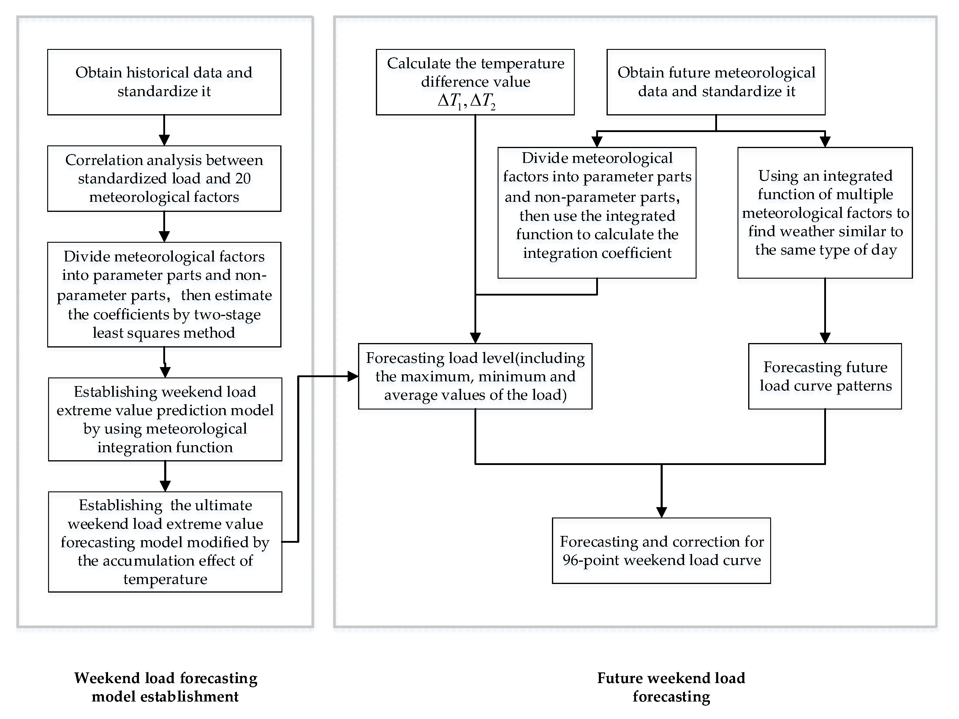
4. Load Forecasting of the Weekend Based on Semi-Parametric Regression

Many factors affect the weekend load change. The same date type makes the sample data have similar characteristics, and the standardization of load weakens the influence of economic growth rate. These make the effect of weather information on weekend load more prominent. To study the load of the weekend, the primary task is to define the acting force of each influencing factor and to determine the elements of the parametric and non-parametric parts of the Semi-parametric model.
The closer the correlation coefficient r is to 1, the more significant the relationship is; the negative r indicates a negative correlation. It could be known from statistics that 0.5 ≤ |r| < 0.8 was considered to be significantly correlated, while 0.3 ≤ |r| < 0.5 was considered to be of low correlation [39]. According to the results of correlation analysis in Table 1, the correlation coefficient 0.5/0.6 was selected as the demarcation point of the independent variable. Then, through the verification of the actual simulation results, the meteorological factors of |r| ≥ 0.5 were finally selected as the independent variables of the parameter part, while the other ones of |r| < 0.5 were the independent variables of the non-parametric part. In this way, the meteorological factors with parametric and non-parametric characteristics can be classified reasonably to establish a Semi-parametric regression model.
There are many kinds of meteorological factors selected. If the coupling relationship between each meteorological factor and load is discussed, the calculation amount will be expanded invisibly. Therefore, it is possible to use the concept of integration to set the effect of each meteorological factor on the weekend to be predicted, and to establish an integral function to calculate the integration coefficients of the parameter and non-parametric parts. Definition of meteorological integration function:
γ = i = 1 n [ | r i i = 1 n r i | ( Y 0 m * Y i m * ) ] 2
where γ is the integration coefficient; Y 0 is the corresponding meteorological standard for the weekend to be predicted; Y i is the corresponding meteorological standard for the first day of the historical day. The steps of weekend load forecasting based on Semi-parametric regression model are as follows:
  • According to the correlation analysis result of each meteorological factor and the load standard value, the standard load of the Semi-parameter can be selected among the independent parameters of the parametric and nonparametric part in the model.
    The independent variables of the parameter part can be expressed as follows:
    x = x 1 , x 2 , x 3 , , x m , m = 1 , 2 , , n
    And the independent variables of the nonparametric part can be expressed as follows:
    z = z 1 , z 2 , z 3 , , z p , p = 1 , 2 , , q
    where n and q are the number of the parametric parts and the non-parametric parts of the meteorological factors, respectively.
  • Standardizing the sample sets of meteorological and load. And integrating the identified meteorological factors that characteristics with parametric and nonparametric by Equation (17).
  • Based on the independent variable of the parametric part, calculating regression coefficient of standardized regression model by least squares, then β * and α * which are the initial estimates of parameters in the Semi-parametric regression model can be obtained.
  • Based on the nonparametric part of the independent variables, establishing the regression model, and calculating the regression coefficient by the least-squares method. The point-by-point residual and its square can be obtained by Equation (11), and the weight W can be calculated by Equation (12).
  • Calculate the g of the non-parametric part at this time by Equation (14).
Based on the data columns (x, y-g) and Equation (15), β * * and α * * which are the final estimates of regression parameters can be obtained by the least squares method.
Utilizing the Semi-parametric regression model to predict the weekend load. The effects of meteorological factors on load are divided into two parts with parametric and non-parametric characteristics, that is, the information with a clear relation to meteorology is considered, and the effect of interfering meteorological factors is not neglected.

5. Temperature Accumulation Effect Correction

The accumulation effect affects the load change in a variety of forms. The typical form is shown as follows: if a place is in high temperature for a long time, the load in this area will be at a higher level. In this case, even if the temperature is reduced, the extent of the load reduction is not obvious. Conversely, when the cool weather continues for a certain period, even if the temperature suddenly rises to a higher level, the load rise is not obvious. The phenomenon that the load lags behind the temperature change is called the temperature accumulation effect. Generally speaking, the occurrence of the accumulation effect of temperature needs to satisfy the condition that the daily temperature to be predicted is in the temperature range sensitive to human perception. Moreover, the intensity of the accumulation effect of temperature is not only affected by the predicted daily temperature but also closely related to the difference between the predicted daily temperature and the temperature of the previous N days. The greater the temperature difference is, the greater the accumulation effect of temperature on the day to be predicted is; however, when the temperature difference exceeds a certain range, the accumulation effect of temperature will gradually weaken [26].
The weekend load level, which is more sensitive to weather factors, is lower than those of normal working days. The accumulation of high temperature or low temperature during the first few days of the weekend will act on the forecasting weekend. Therefore, the load change to be predicted over the weekend is not only affected by the current meteorological changes but also superimposed on the effects of the previous day’s temperature accumulation effect. Assuming that the weekend normal load forecasting model is accurate, the deviation between the forecasting load and the actual load calculated by the model when the accumulation effect is significant can be considered to be mainly caused by the accumulation effect. Therefore, the modified load modeling of the accumulation effect is actually modeling the above load deviation, and the actual load on the weekend is the superposition of the normal load and the load deviation caused by the accumulation effect.
The strength of the accumulation effect is different under different conditions. The strength of accumulation effect is mainly affected by high temperature, high-temperature duration and the temperature of the weekend to be predicted. Temperature correction is used to reflect the accumulation effect, which can not only reflect the effect of accumulation on load but also make full use of the existing load forecasting model. According to the significant degree of accumulation effect, taking the summer meteorological load data as an example, the data with significant accumulation effect and the data without significant accumulation effect are screened out to facilitate the follow-up analysis. Based on the above analysis, the data of the day and the next day when the daily maximum temperature is between 28 C and 38 C and the temperature rises or falls more than 3 C are selected as the significant data of summer accumulation effect, referred to as an accumulation day. Considering the establishment of the accumulation effect correction model, this paper introduces the temperature deviations amount ΔT.
Take the establishment of a summer accumulation effect correction load model as an example:
Calculate the temperature difference value:
Δ T 1 = T 0 T - 1 , Δ T 2 = T 0 - T 2
where T 0 is the temperature of the day when the temperature mutates; T - 1 and T - 2 are the temperatures of the day and two days before the mutation. The result of this formula, as the input variable of the accumulation effect correction formula, reflects the deviation caused by the perceived inertia of the temperature change.
Taking L 2 as the benchmark, L 0 , L 1 and L 2 can be obtained by the basic load forecasting model, and all load deviation values are calculated as follows:
Δ L = L L
The regression coefficients in the accumulation effect correction formula are obtained by multivariate regression analysis of ΔL, ΔT 1 and ΔT 2 with the least-squares method, and the function fT 1 , ΔT 2 ) which changes with the meteorological index can be obtained.
The expression for binary linear regression is as follows:
f Δ T 1 , Δ T 2 = k 1 Δ T 1 + k 2 Δ T 2 + k 3
Adding the accumulation effect of temperature on the basis of the original prediction model can more effectively show the interaction between meteorological-loads, reflecting the real situation of weekend load, and thus further improving the accuracy of weekend load forecasting.

6. Weekend Load Forecasting Model Construction

In this paper, the weekend load forecasting is divided by quantitative and qualitative analysis into two parts: load level forecasting and load curve model forecasting. The load level includes the maximum, minimum and mean load, taking into account the coupling relationship between meteorological and load and the effect of meteorological accumulation. The load curve model forecasting establishes a weather integration function basing on similar days and takes the weekend with the minimum integration coefficient as the base load curve.

6.1. Forecasting of Weekend Load Level

k j = L w e e k L b a s e K j = x j β * * + α * + i = 1 j 1 W i k j x j β * - α * L w e e k . x = L b a s e × f K j j = 1 , 2 , , n
where K is the dependent variable of the Semi-parametric regression model and L w e e k . x is the initial forecast of the total network area of the weekend adjustment load value.
To fit the coupling relationship between the weather and load, the accumulation effect correction load model is taken into account base on normal load model, and the final actual load model is given as follows:
L w e e k . x = L w e e k . x × f Δ T 1 , Δ T 2
where fT 1 , ΔT 2 ) is the expression function of the temperature accumulation effect.

6.2. Forecasting of Weekend Load Curve Model

In a large amount of historical meteorological data, the meteorological information of the same type of weekend is screened out by clustering, and the meteorological forecasting information is collected and calculated for the weekend forecasting. After standardizing the meteorological information, based on the principle of similar day and considering all the effects of meteorological factors, the integrated function is established to find the same type of day with the most similar weather forecast for the weekend. To weaken the impact of the growth rate on the load forecasting, selecting the 7 weekends before the weekend to be predicted as the range of weather-similar days. When the γ is minimum, that is, the weather information of the similar day is the closest to weekend to be predicted. Then the load curve of the same kind of weekend with the most similar weather is used as the base curve of the forecasting model. When the meteorological variation on the forecast date is larger than the historical range, the method can be continued to trace forward, and the monthly base load can be modified proportionally.

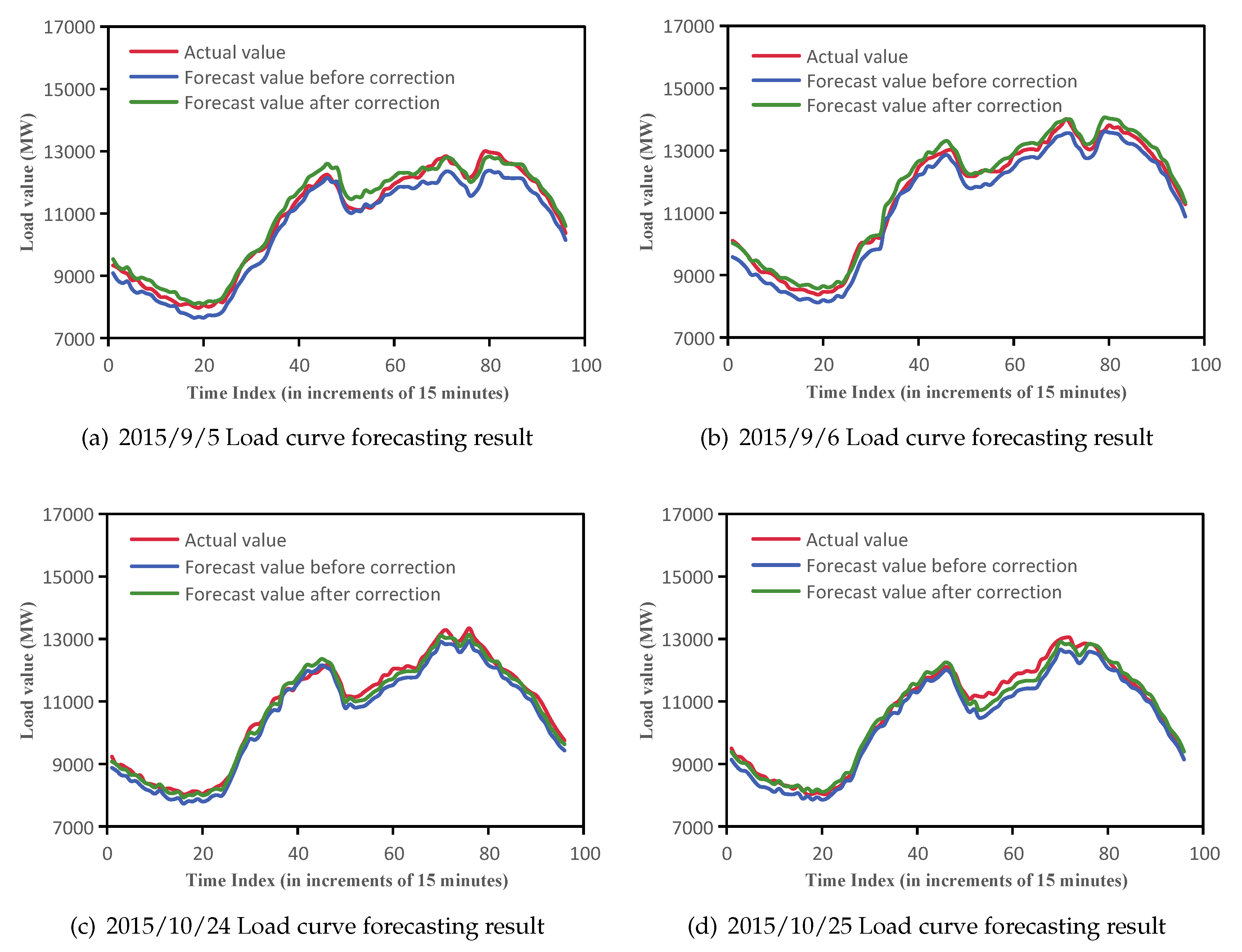
6.3. Forecasting and Correction for 96-Point Weekend Load Curve

The forecasting value of extreme inflection point of weekend load can be obtained using the Semi-parametric regression model and temperature accumulation effect. The final 96-point load curve can be obtained by the optimized correction of the same type of basic load curve obtained by using the meteorological integrated function.
This paper holds that if the deviation of the daily maximum and minimum load of the predicted weekend and similar weather days remain unchanged, then the initial curve Li of the weekend load can be calculated as follows:
L i = S i m L i + L max S i m L max , t > t min S i m L i + L min S i m L min , t < t min L i = L i × L a v e i = 1 n L i
Smoothing the load connection points near the minimum value to avoid burrs in the load curve.
L i = L min + L 08:45 L min × n m n = 1 , 2 , m + 1
where L max , L ave and L min are respectively the maximum, average and minimum load forecasting values of the day to be forecasted; S i m L i is a load curve with similar types of days; S i m L max is the maximum load for similar day; S i m L min is the minimum load for similar day; t min is the minimum point of the corresponding similar daily load curve. m is the total number of load points with 15 min increment in the period from t min to 08:45; and n is the number of load points between L i and L min .
In order to understand more intuitively the process of weekend load forecasting based on semi-parametric regression model of meteorological-load interaction coupling, the forecasting process is listed as shown in Figure 2.

6.4. The Judgment Basis for Load Forecasting Results

Load forecasting is an estimation of the load of the grid in the next few days. The model cannot be completely perfect, and the randomness of external conditions will affect the accuracy of load forecasting. Accuracy is the degree to which the average values measured many times under certain experimental conditions are consistent with the true values. It is used to indicate the magnitude of system errors. Accuracy is the synthesis of systematic error and random error in measurement results, which indicates the consistency between measurement results and true values. The accuracy of the test results consists of accuracy and precision, that is, the accuracy of the test results is reflected by the two indicators of accuracy and precision. Accuracy is often expressed by errors. When used for a set of test results, it consists of random error components (precision) and systematic error components (correctness). Combining with the engineering practice, accuracy A j , relative error E j , mean absolute percentage error (MAPE) and root mean square error (RMSE) are selected as the evaluation basis for the forecasting method:
A j = [ 1 1 n i = 1 n E j 2 ] × 100 % E j = L F i L R i L R i M A P E = 1 n i = 1 n L R i L F i L R i × 100 % R M S E = 1 n i = 1 n L R i L F i 2
where L F i is the load forecast value; L R i is the actual load value; n is the total number of points for daily load forecasting.

7. Specific Example and Results Analysis

7.1. Sample Load Forecasting Based on Semi-Parametric Method

To prove that the proposed Semi-parametric weekend load forecasting method based on the interaction between meteorology and load can accurately predict the load value of the future power grid, the weekend load forecasting model is simulated and tested based on the load data of a southern power grid. Weekend load forecasting model is established based on the data of 2008–2014 as a historical sample set, and the data of 2015 as a test set is selected to test the final results of the forecasting. The weekend load forecasting model is as follows. Table 2 lists the forecasting relative error results of load maximum in 2015 weekend in detail by month.
Weekend load forecasting model:
K j = 0.4403 x j + 0.9916 + i = 1 j 1 W i k j + 0.4399 x j 0.9917 L w e e k . x = L b a s e × f K j L b a s e × f K j j = 1 , 2 , , n L w e e k . x = L w e e k . x 7.6154 Δ T 1 55.1568 Δ T 2 116.9302
The weekend load forecasting method proposed in this paper can also maintain the stability of weekend load forecasting on continuous dates. To prove this advantage, the weekends of September and October of 2015 were selected for verification. Table 3 shows the specific results of continuous weekend load forecasting, in which the A mark , the prediction results of the quadratic regression prediction model, is selected as the benchmark to verify the superiority of the Semi-parametric model; the correlation coefficient r is 0.6 to verify the rationality of the selection of independent variable boundary points; and the accuracy of A before and A after of the 96-point load curve before and after the accumulation effect correction are compared. Also, Figure 3 series diagrams show the actual load tracking and forecasting values of the weekend.
As can be seen from Table 2 the annual error rate of the maximum load on the weekend of 2015 is 0.0252. The average accuracy of the 9–10-month continuous weekend 96-point load curve selected from Table 3 shows that the weekend load forecasting curve obtained by the Semi-parametric model used in this paper is closer to the actual value load curve than the regression model. The correlation coefficient selection 0.5 with an average accuracy of 97.06% is more advantageous than 0.6 with an average accuracy of 96.76% as a whole, and the forecasting accuracy after the accumulation effect correction is improved obviously, the accuracy was 97.06% before correction, and can reach 98.15% after the correction. Figure 3 also shows that the continuous weekend load forecasting curve can well track the actual value, which proves that the proposed weekend load forecasting method has strong stability. It can be concluded that the proposed Semi-parametric weekend load forecasting method based on weather-load interaction can meet the requirements of load forecasting accuracy of the power grid and meet the actual operation needs of the power grid.

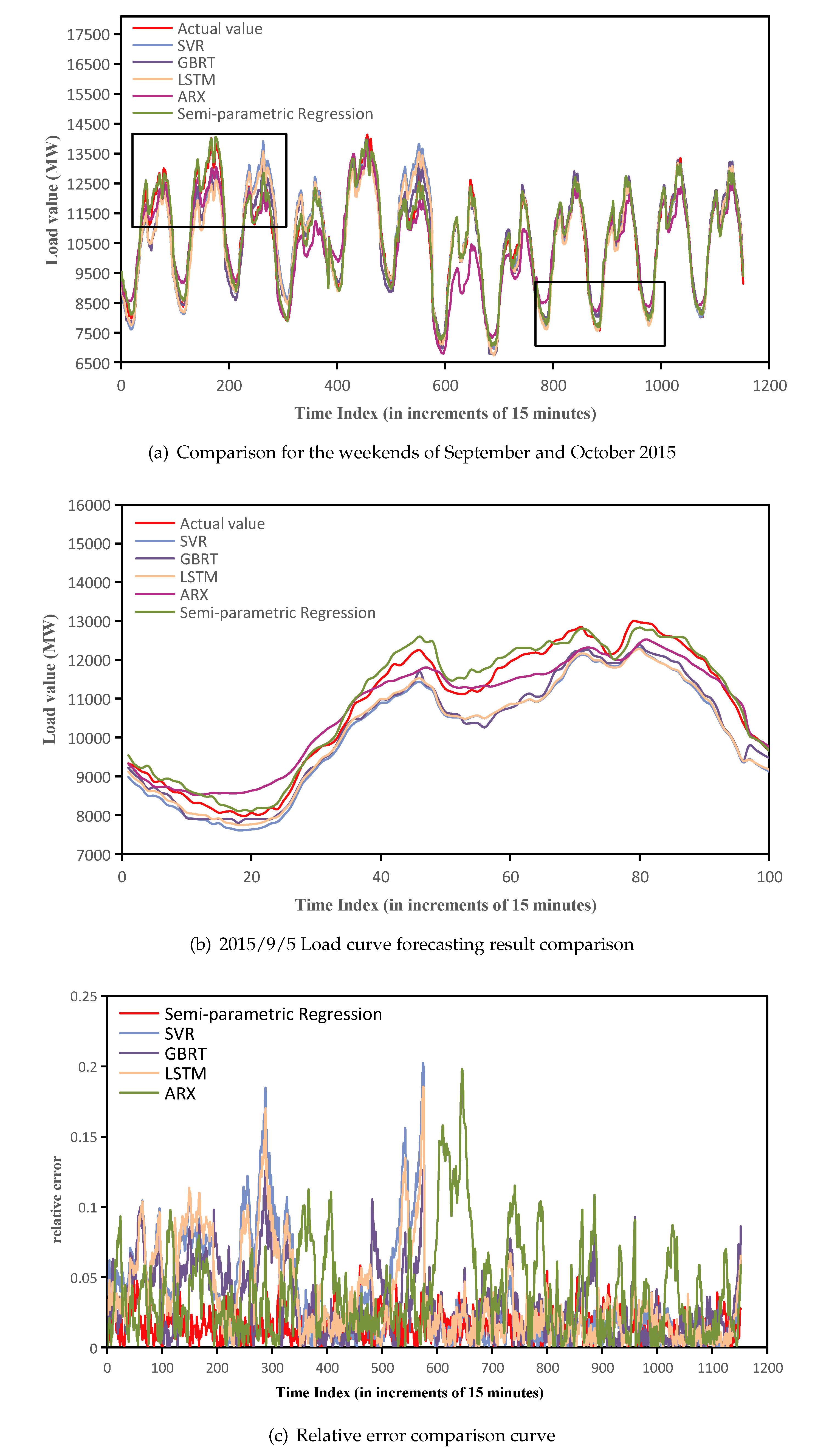
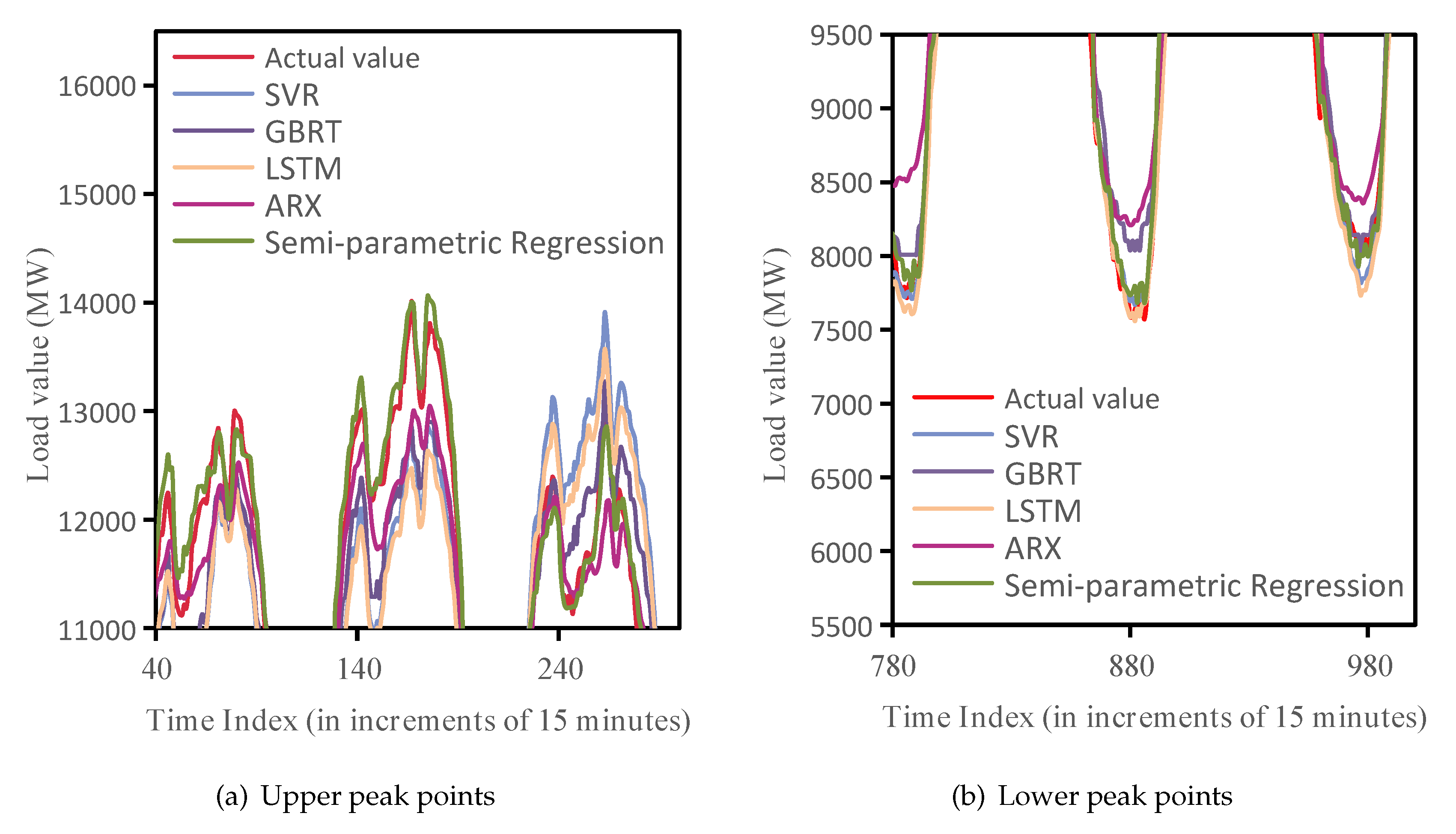
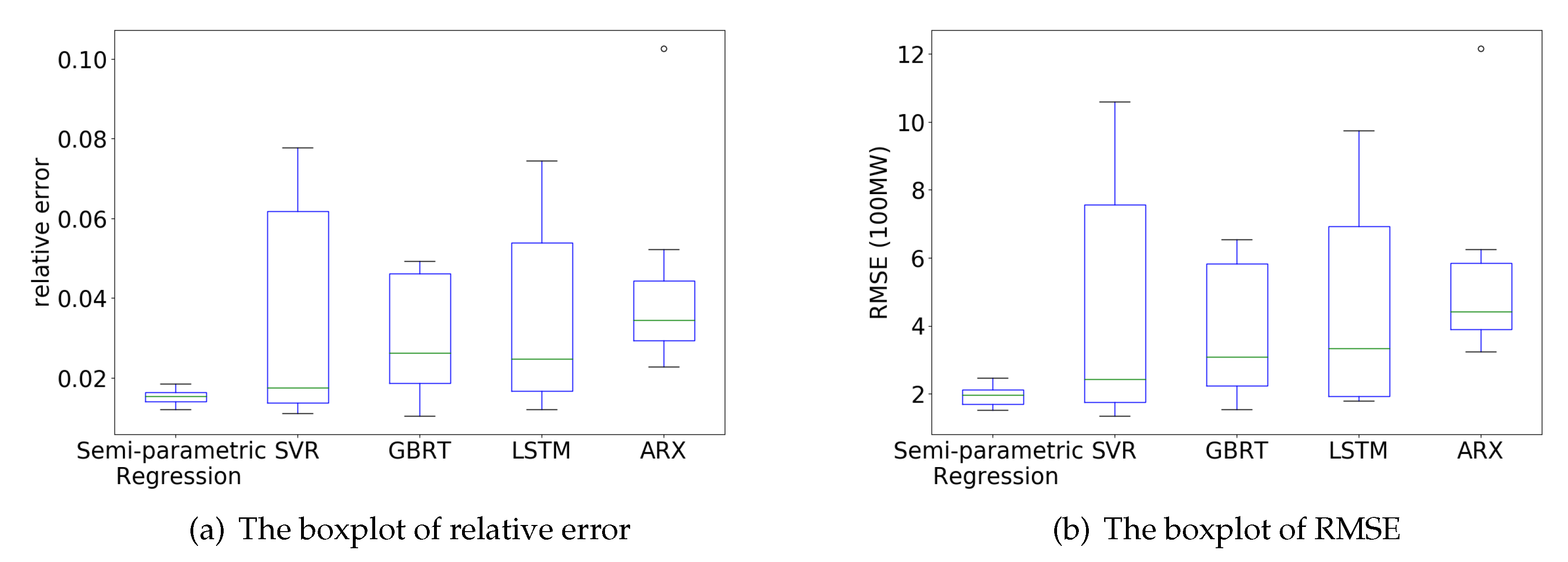
7.2. Comparison and Analysis of Model Prediction Results

To verify the effect of the proposed Semi-parametric weekend-load forecasting method based on the interaction between meteorological and load, the Long Short-Term Memory (LSTM) model [40], the traditional Support Vector Regression (SVR) model [41], the Gradient Boosting Regression Tree (GBRT) model [42] and the Auto-Regressive eXogenous (ARX) model [43] are selected for comparison, predicting the load values in the same 12 weekend days. The comparison of forecasting results, the relative error and the boxplot of relative error for different models are shown in Figure 4, Figure 5 and Figure 6 respectively.
For the weekends of September and October 2015 data set, The fitting results of the forecasting curves for each model are presented in Figure 4a,b. Obviously, the forecasting curve of the Semi-parametric Regression model fits best. As can be seen from Figure 4c, for the samples, the Semi-parametric Regression model improves the prediction accuracy at most of sharp points. The local details for sharp points in Figure 4a are enlarged and are shown in Figure 5a,b respectively. From the enlarged figure, the proposed Semi-parametric weekend-load forecasting method is superior to other models on the upper and lower peak points, not only in terms of the fitting degree but also in terms of the trend shape.
The boxplot in Figure 6 shows the four statistics of the relative error and RMSE of each forecasting model that is the minimum, first quartile, the median, third quartile and the maximum. It indicates that the relative error distribution range of the proposed Semi-parametric Regression model is always the smallest compared with other models, and so is the RMSE. As shown in Table 4, the mean absolute percentage errors (MAPE) for the 15 min load of each forecasting day of the Semi-parametric Regression model are the most stable and reliable. It is proved that the Semi-parametric Regression model proposed in this paper can achieve good prediction effect in weekend load short-term forecasting.

8. Conclusions

This paper proposes a Semi-parametric weekend load forecasting method, which uses the interaction between meteorology and load to effectively improve the accuracy of weekend load forecasting. Its innovations are as follows:
1. Applying the Semi-parametric forecasting model to short-term load forecasting. Many meteorological factors are divided into two categories with parametric characteristics and non-parametric characteristics. In this way, information that has a clear relationship with meteorology is considered without ignoring the effects of interfering meteorological factors.
2. This paper presents the concept of integration in which the effect of meteorological factors on the forecasting weekend is expressed by establishing the integration function to calculate the integration coefficient of the parametric part and non-parameter part. Also, the method of normalization is proposed to fuzzify the meteorology and screen out the interference of the meteorological numerical difference on the meteorological similarity search, to guarantee the validity of the meteorological integrated function to a great extent.
The proposed weekend load forecasting method has certain applicability to the regional power network of China and does not take the regional characteristics into account for special treatment. However, national holidays and typhoon days are excluded in the actual modeling, so it is necessary to further study the effect of multi-date type overlapping and typhoon destruction on power grid load to improve the accuracy of all-weather load forecasting.

Author Contributions

B.L. proposed the concept of this research and provided guidance and writing; M.L. carried on data analysis and writing; J.H. made further modification on this paper; Y.Z. provided guidance and made further modification on this paper.

Funding

This research was funded by the National Natural Science Foundation of China (51767004), the Guangxi scientific research and technology development project (1599005-2-14), and the Natural Science Foundation of Guangxi (2018JJB160056; 2018JJB160064; 2018JJA160176).

Acknowledgments

This project was supported by National Natural Science Foundation of China (51767004), the Guangxi scientific research and technology development project (1599005-2-14), the Natural Science Foundation of Guangxi (2018JJB160056; 2018JJB160064; 2018JJA160176), the Guangxi thousand backbone teachers training program, the boshike award scheme for young innovative talents, and the Guangxi bagui young scholars special funding.

Conflicts of Interest

The authors declare no conflict of interest.

References

  1. Gao, C.; Li, Q.; Su, W.; Li, Y. Temperature correction model research considering temperature cumula-tive effect in short-term load forecasting. Trans. China Electromech. Soc. 2015, 30, 242–248. [Google Scholar]
  2. Li, C.; Yang, P.; Liu, W.; Li, D.; Wang, Y. An analysis of ac-accumulation effect of temperature in short-term load fore-casting. Autom. Electr. Power Syst. 2009, 33, 96–99. [Google Scholar]
  3. Buitrago, J.; Asfour, S. Short-Term Forecasting of Electric Loads Using Nonlinear Autoregressive Artificial Neural Networks with Exogenous Vector Inputs. Energies 2017, 10, 40. [Google Scholar] [CrossRef]
  4. Bennett, C.; Stewart, R.A.; Lu, J.W. Autoregressive with Exogenous Variables and Neural Network Short-Term Load Forecast Models for Residential Low Voltage Distribution Networks. Energies 2014, 7, 2938–2960. [Google Scholar] [CrossRef]
  5. Tian, C.S.; Hao, Y. A Novel Nonlinear Combined Forecasting System for Short-Term Load Forecasting. Energies 2018, 11, 712. [Google Scholar] [CrossRef]
  6. Cai, G.W.; Wang, W.J.; Lu, J.H. A Novel Hybrid Short Term Load Forecasting Model Considering the Error of Numerical Weather Prediction. Energies 2016, 9, 994. [Google Scholar] [CrossRef]
  7. Niu, D.X.; Dai, S.Y. A Short-Term Load Forecasting Model with a Modified Particle Swarm Optimization Algorithm and Least Squares Support Vector Machine Based on the Denoising Method of Empirical Mode Decomposition and Grey Relational Analysis. Energies 2017, 10, 408. [Google Scholar] [CrossRef]
  8. Hong, W.C.; Fan, G.F. Hybrid Empirical Mode Decomposition with Support Vector Regression Model for Short Term Load Forecasting. Energies 2019, 12, 1093. [Google Scholar] [CrossRef]
  9. Al-Musaylh, M.S.; Deo, R.C.; Li, Y.; Adamowski, J.F. Two-phase particle swarm optimized-support vector regression hybrid model integrated with improved empirical mode decomposition with adaptive noise for multiple-horizon electricity demand forecasting. Appl. Energy 2018, 217, 422–439. [Google Scholar] [CrossRef]
  10. Liu, T.X.; Jin, Y.; Gao, Y.Y. A New Hybrid Approach for Short-Term Electric Load Forecasting Applying Support Vector Machine with Ensemble Empirical Mode Decomposition and Whale Optimization. Energies 2019, 12, 1520. [Google Scholar] [CrossRef]
  11. Wu, X.; He, J.; Zhang, P.; Hu, J. Power system short-term load forecasting based on improved random forest with grey relation projection. Autom. Electr. Power Syst. 2015, 39, 50–55. [Google Scholar]
  12. Wu, X.; He, J.; Yip, T.; Jian, L.; Ning, L. A two-stage random forest method for short-term load forecasting. In Proceedings of the Power & Energy Society General Meeting, Boston, MA, USA, 17–21 July 2016. [Google Scholar]
  13. Moon, J.; Kim, Y.; Son, M.; Hwang, E. Hybrid Short-Term Load Forecasting Scheme Using Random Forest and Multilayer Perceptron. Energies 2018, 11, 3283. [Google Scholar] [CrossRef]
  14. Chen, M.; Yuan, J.; Liu, D.; Tao, L. An adaption scheduling based on dynamic weighted random forests for load demand forecasting. J. Supercomput. 2017, 1–19. [Google Scholar] [CrossRef]
  15. Kong, W.; Zhao, Y.D.; Hill, D.J.; Luo, F.; Yan, X. Short-Term Residential Load Forecasting based on Resident Behaviour Learning. IEEE Trans. Power Syst. 2017, 33, 1087–1088. [Google Scholar] [CrossRef]
  16. Wang, S.X.; Wang, X.; Wang, S.M.; Wang, D. Bi-directional long short-term memory method based on attention mechanism and rolling update for short-term load forecasting. Int. J. Electr. Power Energy Syst. 2019, 109, 470–479. [Google Scholar] [CrossRef]
  17. Kuo, P.H.; Huang, C.J. A High Precision Artificial Neural Networks Model for Short-Term Energy Load Forecasting. Energies 2018, 11, 213. [Google Scholar] [CrossRef]
  18. Feng, Y.; Xu, X.F.; Meng, Y. Short-Term Load Forecasting with Tensor Partial Least Squares-Neural Network. Energies 2019, 12, 990. [Google Scholar] [CrossRef]
  19. Fallah, S.N.; Ganjkhani, M.; Shamshirband, S.; Chau, K.W. Computational Intelligence on Short-Term Load Forecasting: A Methodological Overview. Energies 2019, 12, 393. [Google Scholar] [CrossRef]
  20. Bouktif, S.; Fiaz, A.; Ouni, A.; Serhani, M.A. Single and Multi-Sequence Deep Learning Models for Short and Medium Term Electric Load Forecasting. Energies 2019, 12, 149. [Google Scholar] [CrossRef]
  21. Jiao, R.H.; Su, C.J.; Lin, B.Y.; Mo, R.F. Short Term-Load Forecasting Based on Meteorological Correcting Grey Model. In Unifying Electrical Engineering and Electronics Engineering; Springer: New York, NY, USA, 2014. [Google Scholar]
  22. Li, G.D.; Wang, C.H.; Masuda, S.; Nagai, M. A research on short term load forecasting problem applying improved grey dynamic model. Int. J. Electr. Power Energy Syst. 2011, 33, 809–816. [Google Scholar] [CrossRef]
  23. Wang, H.; Yang, K.; Xue, L.Y.; Shuang, L. The Study of Long-term Electricity Load Forecasting Based on Improved Grey Prediction. In Proceedings of the International Conference on Machine Learning & Cybernetics, Tianjin, China, 14–17 July 2013. [Google Scholar]
  24. Zhang, Y. The Application of Semi-parametric Re-gression Model in Long-middle Term Load Forecast-ing. In Power System and Its Automation School of Electrical Engineering; Zhengzhou University: Zhengzhou, China, 2010. [Google Scholar]
  25. Goude, Y.; Nedellec, R.; Kong, N. Local Short and Middle Term Electricity Load Forecasting With Semi-Parametric Additive Models. IEEE Trans. Smart Grid 2014, 5, 440–446. [Google Scholar] [CrossRef]
  26. Li, J.; Li, X.; Liu, S. Short-term Load Forecasting Considering the Acaccumulation effects of Tem-peratures. IEEE Trans. Smart Grid 2013, 40, 49–54. [Google Scholar]
  27. Gregorczuk, M.; Cena, K. Distribution of Effective Temperature over the surface of the Earth. Int. J. Biometeorol. 1967, 11, 145–149. [Google Scholar] [CrossRef]
  28. Du, Y.; Lin, L.; Mou, D.; He, X. Analysis of the Impact of Comprehensive Meteorological Index on Electric Power Load. J. Chongqing Univ. 2006, 29, 56–60. [Google Scholar]
  29. Tromp, S.W. Medical Biometeorology; Elsevier: Amsterdam, The Netherlands, 1963. [Google Scholar]
  30. Zar, J.H. Significance Testing of the Spearman Rank Correlation Coefficient. Publ. Am. Stat. Assoc. 1972, 67, 578–580. [Google Scholar] [CrossRef]
  31. Spearman, C. The proof and measurement of association between two things. Am. J. Psychol. 1987, 100, 441–471. [Google Scholar] [CrossRef] [PubMed]
  32. Zhang, Y.; Li, X.; Zheng, H.; Yao, H.; Liu, J.; Zhang, C.; Peng, H.; Jiao, J. A Fault Diagnosis Model of Power Transformers Based on Dissolved Gas Analysis Features Selection and Improved Krill Herd Algorithm Optimized Support Vector Machine. IEEE Access 2019, 7, 102803–102811. [Google Scholar] [CrossRef]
  33. Dong, Y.; Zhang, Z.; Hong, W.C. A Hybrid Seasonal Mechanism with a Chaotic Cuckoo Search Algorithm with a Support Vector Regression Model for Electric Load Forecasting. Energies 2018, 11, 1009. [Google Scholar] [CrossRef]
  34. Ma, S.; Chen, X.; Liao, Y.; Gang, W.; Ding, X.; Kai, C. The variable weight combination load forecasting based on grey model and semi-parametric Regression Model. In Proceedings of the Tencon IEEE Region 10 Conference, Xi’an, China, 22–25 October 2013. [Google Scholar]
  35. Wang, X.; Chen, Z.; Yang, S. Forecasting modeling and simulation analysis of a power system in China, based on a class of Semi-parametric regression ap-proach. S. Afr. J. Ind. Eng. 2012, 23, 154–168. [Google Scholar]
  36. Ferraty, F.; Goia, A.; Salinelli, E.; Vieu, P. Peak-Load Forecasting Using a Functional Semi-Parametric Approach. In Topics in Nonparametric Statistics; Springer: New York, NY, USA, 2014. [Google Scholar]
  37. Robinson, P.M. Root-N-Consistent Semiparametric Regression. Econometrica 1988, 56, 931–954. [Google Scholar] [CrossRef]
  38. Li, Q. Nonparametric Econometrics: Theory and Practice; Princeton University Press: Princeton, NJ, USA, 2007. [Google Scholar]
  39. Li, J.; Qi, X. Principles of Statistics, 3rd ed.; Shanghai Fudan University Press: Shanghai, China, 2005; pp. 340–341. [Google Scholar]
  40. Kong, W.; Dong, Z.Y.; Jia, Y.; Hill, D.J.; Zhang, Y. Short-Term Residential Load Forecasting based on LSTM Recurrent Neural Network. IEEE Trans. Smart Grid 2017, 10, 841–851. [Google Scholar] [CrossRef]
  41. Fattaheian-Dehkordi, S.; Fereidunian, A.; Gholami-Dehkordi, H.; Lesani, H. Hour-ahead demand forecasting in smart grid using support vector regression (SVR). Int. Trans. Electr. Energy Syst. 2015, 24, 1650–1663. [Google Scholar] [CrossRef]
  42. Papadopoulos, S.; Karakatsanis, I. Short-term electricity load forecasting using time series and ensemble learning methods. In Proceedings of the 2015 IEEE Power and Energy Conference at Illinois (PECI), Champaign, IL, USA, 20–21 February 2015. [Google Scholar]
  43. Guo, Y.; Nazarian, E.; Ko, J.; Rajurkar, K. Hourly cooling load forecasting using time-indexed ARX models with two-stage weighted least squares regression. Energy Convers. Manag. 2014, 80, 46–53. [Google Scholar] [CrossRef]
Figure 1. Comparison of weekend load and weekday load characteristics.
Energies 12 03820 g001
Figure 2. The flowchart of weekend forecasting.
Energies 12 03820 g002
Figure 3. Forecasting curves compared with the actual load curve in 2015 weekend.
Energies 12 03820 g003
Figure 4. The comparison of forecasting result.
Energies 12 03820 g004
Figure 5. The comparison of forecasting result.
Energies 12 03820 g005
Figure 6. The boxplot of relative error and root mean square error (RMSE) for different models.
Energies 12 03820 g006
Table 1. Summer and winter holiday daily maximum load per-unit value and 20 meteorological factors of correlation.
Meteorological FactorsSummer CorrelationWinter Correlation
Maximum temperature0.7554 **−0.6415 **
Mean temperature0.7637 **−0.6372 **
Minimum temperature0.6651 **−0.5678 **
Maximum humidity−0.3972 **−0.1061
Mean humidity−0.5036 **0.0078
Minimum humidity−0.5382 **0.0878
Average wind speed−0.04500.1614 **
Rainfall−0.3607 **0.1039 **
Maximum temperature humidity index0.7159 **−0.6375 **
Mean temperature humidity index0.6754 **−0.6342 **
Minimum temperature humidity index0.3520 **−0.5797 **
Maximum effective temperature0.7373 **−0.6236 **
Mean effective temperature0.7260 **−0.6226 **
Minimum effective temperature0.5501 **−0.5683 **
Maximum comfort index0.6744 **−0.6173 **
Mean comfort index0.6253 **−0.6114 **
Minimum comfort index0.3438 **−0.5618 **
Maximum chillness humidity index−0.7569 **0.6321 **
Mean chillness humidity index−0.7642 **0.6257 **
Minimum chillness humidity index−0.6744 **0.5662 **
** represents that the correlation was significant at 0.01 level(two-sided).
Table 2. Relative Error of Load Maximum Forecasting Results in 2015 Weekend.
MonthJanuaryFebruaryMarchApril
E j 0.02740.02930.02680.0214
MonthMayJuneJulyAugust
E j 0.02590.02870.02930.0264
MonthSeptemberOctoberNovemberDecember
E j 0.01530.02290.02960.0197
Table 3. Weekend Load Curve Forecast Results in 2015.
DateActual ValueForecasting ValueA mark A before - 0.6 A before - 0.5 A after - 0.5
MaxMeanMinMaxMeanMin
9/513,00210,797797312,83210,727820296.26%96.99%96.81%97.85%
9/614,01411,556837114,46311,605856995.95%96.98%97.11%98.20%
9/1212,87510,986895912,55710,713869295.23%96.71%96.50%97.81%
9/1312,37310,227791812,35110,592817995.38%95.99%97.10%98.32%
9/1914,13311,885901814,19012,108928195.61%96.92%97.01%98.04%
9/2012,77410,997920412,55810,704897896.81%96.58%96.64%98.23%
10/1012,6149755715212,4019706732494.32%95.91%97.11%98.11%
10/1112,0199535697712,2409826724796.30%96.88%97.39%98.37%
10/1712,78910,354771612,87510,722796995.51%96.84%97.64%97.87%
10/1812,48010,175757112,74010,478778296.33%97.04%97.26%98.03%
10/2413,34410,768802512,87710,207779897.06%97.31%97.12%98.57%
10/2513,04610,661801612,84010,665810596.53%96.98%97.05%98.36%
Table 4. Mean absolute percentage errors (MAPE) of Weekend Load Curve Forecast Results of September and October in 2015.
DateSVRGBRTLSTMARXSemi-Parametric
Regression
5 September 20156.01%4.92%5.31%3.22%1.84%
6 September 20156.88%4.58%7.44%4.44%1.54%
12 September 20156.70%4.74%5.59%2.39%1.21%
13 September 20155.93%4.13%4.88%4.43%1.40%
19 September 20151.91%1.39%2.92%3.52%1.53%
20 September 20157.78%4.87%6.37%2.79%1.62%
10 October 20151.57%1.88%1.60%10.26%1.59%
11 October 20151.57%2.71%2.01%5.23%1.41%
17 October 20151.11%1.82%1.68%3.71%1.76%
18 October 20151.37%2.54%1.73%3.35%1.68%
24 October 20151.36%1.04%1.58%2.98%1.22%
25 October 20151.18%2.02%1.20%2.28%1.40%

