Comparison of LSSVR, M5RT, NF-GP, and NF-SC Models for Predictions of Hourly Wind Speed and Wind Power Based on Cross-Validation

 ,
, 


Abstract
1. Introduction
2. Methods Applied in the Research
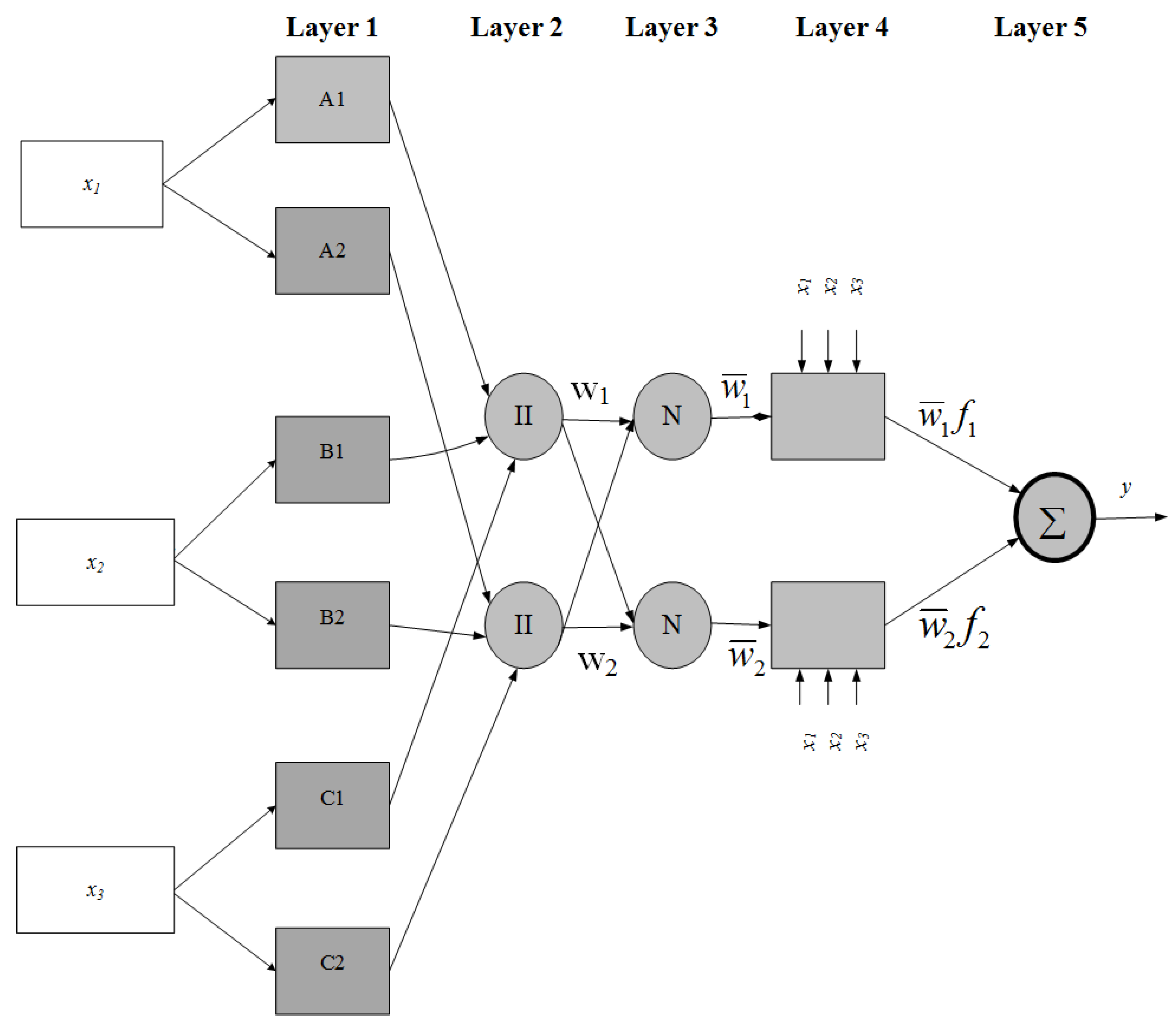
2.1. Neuro-Fuzzy System
2.2. Least Square Support Vector Regression
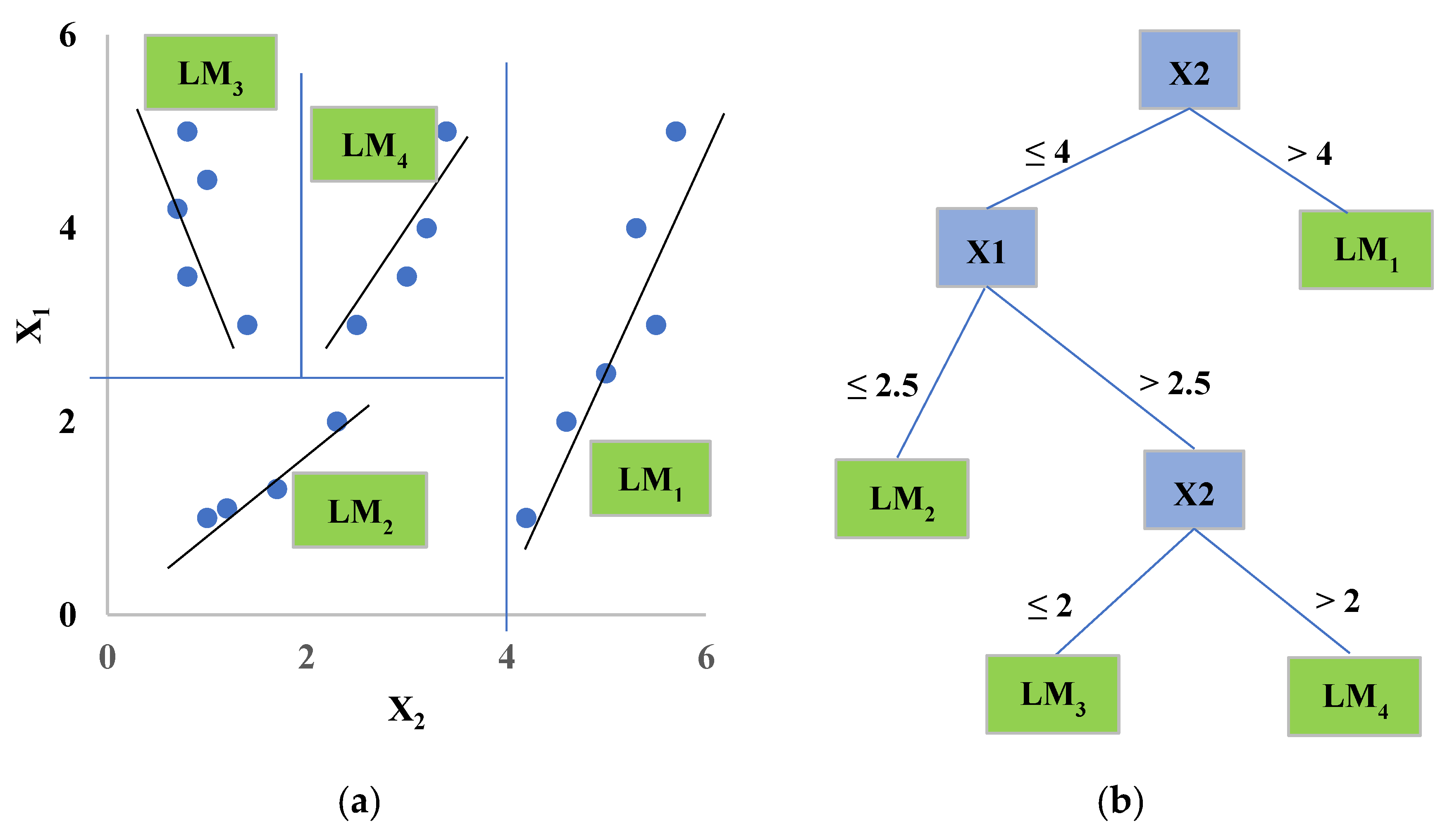
2.3. M5RT
3. Dataset and Statistical Analysis
4. Results and Discussion
4.1. Hourly Wind Speed Prediction Using NF-SC, NF-GP, LSSVR, and M5RT Methods
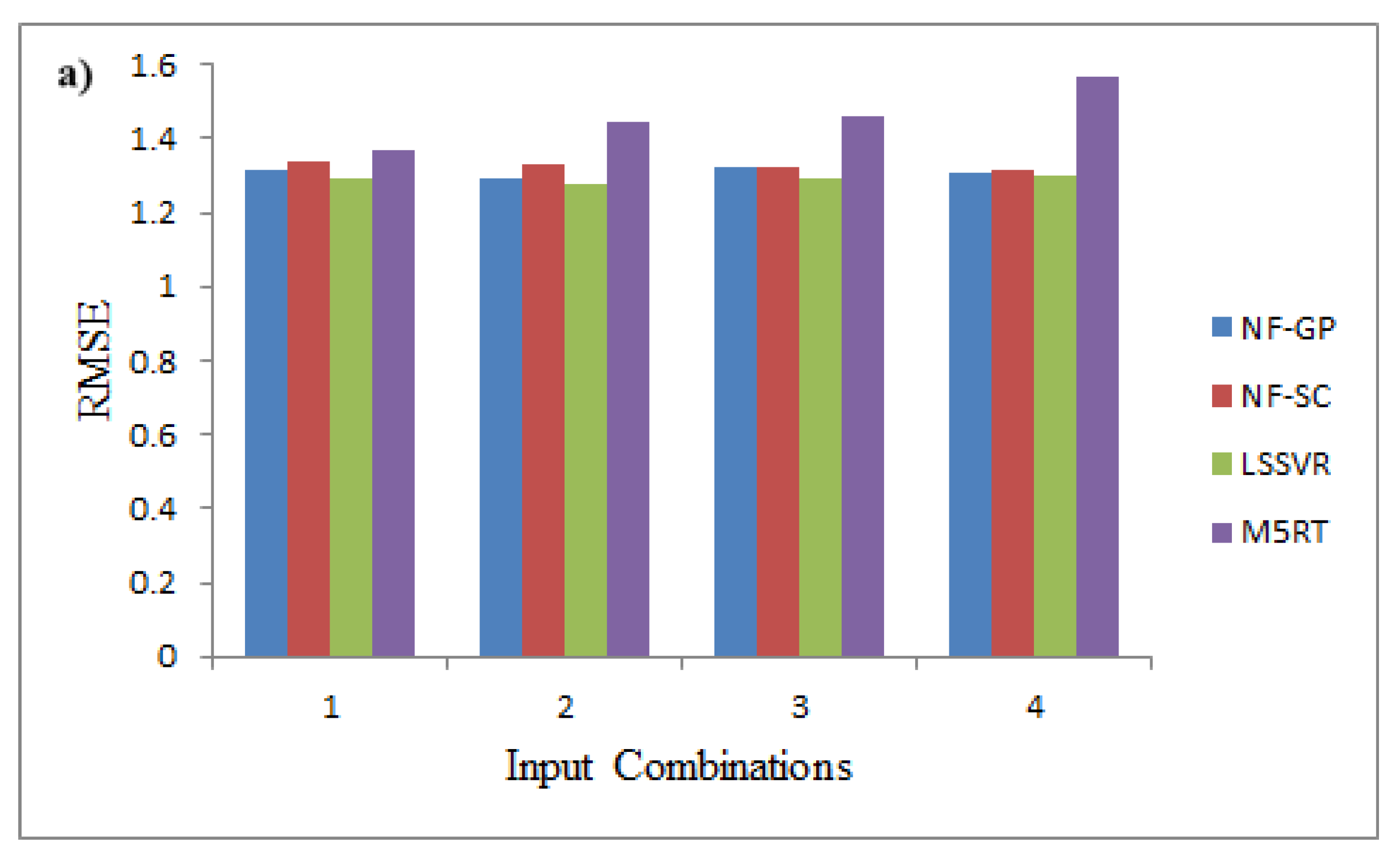
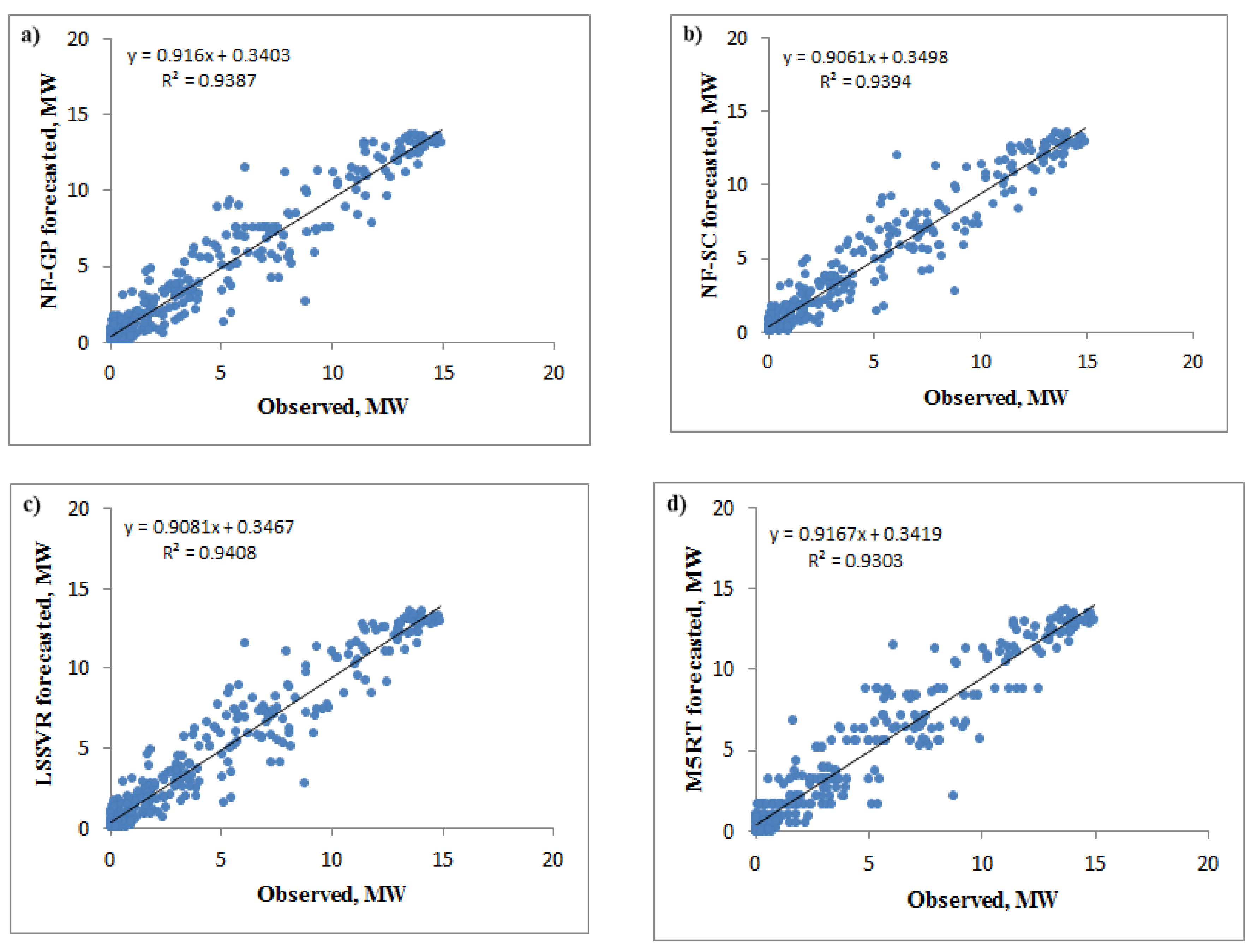
4.2. Hourly Wind Power Prediction Using NF-SC, NF-GP, LSSVR, and M5RT Methods
5. Conclusions
Author Contributions
Funding
Acknowledgments
Conflicts of Interest
References
- Angelis-Dimakis, A.; Biberacher, M.; Dominguez, J.; Fiorese, G.; Gadocha, S.; Gnansounou, E.; Guariso, G.; Kartalidis, A.; Panichelli, L.; Pinedo, I.; et al. Methods and tools to evaluate the availability of renewable energy sources. Renew. Sustain. Energy Rev. 2011, 15, 1182–1200. [Google Scholar] [CrossRef]
- World Wind Energy Association. Wind Power Capacity Reaches 539 GW, 52,6 GW Added in 2017. Available online: http:// wwindea.org/blog/2018/02/12/2017-statistics/ (accessed on 22 December 2018).
- Yuan, X.; Tian, H.; Yuan, Y.; Huang, Y.; Ikram, R.M. An extended NSGA-III for solution multi-objective hydro-thermal-wind scheduling considering wind power cost. Energy Convers. Manag. 2015, 96, 568–578. [Google Scholar] [CrossRef]
- Alessandrini, S.; Delle Monache, L.; Sperati, S.; Nissen, J. A novel application of an analog ensemble for short-term wind power forecasting. Renew. Energy 2015, 76, 768–781. [Google Scholar] [CrossRef]
- Yesilbudak, M.; Sagiroglu, S.; Colak, I. A new approach to very short term wind speed prediction using k-nearest neighbor classification. Energy Convers. Manag. 2013, 69, 77–86. [Google Scholar] [CrossRef]
- Jung, J.; Broadwater, R.P. Current status and future advances for wind speed and power forecasting. Renew. Sustain. Energy Rev. 2014, 31, 762–777. [Google Scholar] [CrossRef]
- Togelou, A.; Sideratos, G.; Hatziargyriou, N.D. Wind power forecasting in the absence of historical data. IEEE Trans. Sustain. Energy 2012, 3, 416–421. [Google Scholar] [CrossRef]
- Fortuna, L.; Nunnari, S.; Guariso, G. Fractal order evidences in wind speed time series. In Proceedings of the ICFDA’14 International Conference on Fractional Differentiation and Its Applications 2014, Catania, Italy, 23–25 June 2014; pp. 1–6. [Google Scholar]
- Torres, J.L.; Garcia, A.; De Blas, M.; De Francisco, A. Forecast of hourly average wind speed with arma models in navarre (spain). Sol. Energy 2005, 79, 65–77. [Google Scholar] [CrossRef]
- Cadenas, E.; Rivera, W. Wind speed forecasting in the south coast of Oaxaca, Mexico. Renew. Energy 2007, 32, 2116–2128. [Google Scholar] [CrossRef]
- Fortuna, L.; Guariso, G.; Nunnari, S. One Day Ahead Prediction of Wind Speed Class by Statistical Models. Int. J. Renew. Energy Res. 2016, 6, 1137–1145. [Google Scholar]
- Fortuna, L.; Nunnari, G.; Nunnari, S. A new fine-grained classification strategy for solar daily radiation patterns. Pattern Recognit. Lett. 2016, 81, 110–117. [Google Scholar] [CrossRef]
- Fortuna, L.; Nunnari, S.; Guariso, G. One day ahead prediction of wind speed class. In Proceedings of the 2015 International Conference on Renewable Energy Research and Applications (ICRERA), Palermo, Italy, 22–25 November 2015; pp. 965–970. [Google Scholar]
- Kavasseri, R.G.; Seetharaman, K. Day-ahead wind speed forecasting using f-ARIMA models. Renew. Energy 2009, 34, 1388–1393. [Google Scholar] [CrossRef]
- Erdem, E.; Shi, J. ARMA based approaches for forecasting the tuple of wind speed and direction. Appl. Energy 2011, 88, 1405–1414. [Google Scholar] [CrossRef]
- Osório, G.; Matias, J.; Catalão, J. Short-term wind power forecasting using adaptive neuro-fuzzy inference system combined with evolutionary particle swarm optimization, wavelet transform and mutual information. Renew. Energy 2015, 75, 301–307. [Google Scholar] [CrossRef]
- Muhammad Adnan, R.; Yuan, X.; Kisi, O.; Yuan, Y.; Tayyab, M.; Lei, X. Application of soft computing models in streamflow forecasting. In Proceedings of the Institution of Civil Engineers-Water Management, London, UK, 30 October 2017; pp. 1–12. [Google Scholar]
- Hu, J.; Wang, J.; Zeng, G. A hybrid forecasting approach applied to wind speed time series. Renew. Energy 2013, 60, 185–194. [Google Scholar] [CrossRef]
- Cadenas, E.; Rivera, W. Short term wind speed forecasting in La Venta, Oaxaca, México, using artificial neural networks. Renew. Energy 2009, 34, 274–278. [Google Scholar] [CrossRef]
- Calif, R.; Schmitt, F.G. Modeling of atmospheric wind speed sequence using a lognormal continuous stochastic equation. J. Wind Eng. Ind. Aerodyn. 2012, 109, 1–8. [Google Scholar] [CrossRef]
- Calif, R.; Schmitt, F.G.; Huang, Y. Multifractal description of wind power fluctuations using arbitrary order Hilbert spectral analysis. Phys. A Stat. Mech. Appl. 2013, 392, 4106–4120. [Google Scholar] [CrossRef]
- Duran Medina, O.; Schmitt, F.G.; Calif, R. Scaling forecast models for wind turbulence and wind turbine power intermittency. In Proceedings of the 19th EGU General Assembly Conference Abstracts, Vienna, Austria, 23–28 April 2017; Volume 19, p. 10374. [Google Scholar]
- Kisi, O.; Parmar, K.S. Application of least square support vector machine and multivariate adaptive regression spline models in long term prediction of river water pollution. J. Hydrol. 2016, 534, 104–112. [Google Scholar] [CrossRef]
- Kisi, O.; Shiri, J.; Karimi, S.; Adnan, R.M. Three different adaptive neuro fuzzy computing techniques for forecasting long-period daily streamflows. In Big Data in Engineering Applications; Springer: Singapore, 2018; pp. 303–321. [Google Scholar]
- Castellanos, F.; James, N. Average hourly wind speed forecasting with ANFIS. In Proceedings of the 11th American Conference on Wind Engineering, San Juan, Puerto Rico, 22–26 June 2009. [Google Scholar]
- Liu, H.; Tian, H.Q.; Li, Y.F. Comparison of new hybrid FEEMD-MLP, FEEMD-ANFIS, Wavelet Packet-MLP and Wavelet Packet-ANFIS for wind speed predictions. Energy Convers. Manag. 2015, 89, 1–11. [Google Scholar] [CrossRef]
- Saleh, A.E.; Moustafa, M.S.; Abo-Al-Ez, K.M.; Abdullah, A.A. A hybrid neuro-fuzzy power prediction system for wind energy generation. Int. J. Electr. Power Energy Syst. 2016, 74, 384–395. [Google Scholar] [CrossRef]
- De Giorgi, M.G.; Ficarella, A.; Tarantino, M. Error analysis of short term wind power prediction models. Appl. Energy 2011, 88, 1298–1311. [Google Scholar] [CrossRef]
- Mohandes, M.; Rehman, S.; Rahman, S. Estimation of wind speed profile using adaptive neuro-fuzzy inference system (ANFIS). Appl. Energy 2011, 88, 4024–4032. [Google Scholar] [CrossRef]
- Sfetsos, A. A comparison of various forecasting techniques applied to mean hourly wind speed time series. Renew. Energy 2000, 21, 23–35. [Google Scholar] [CrossRef]
- Johnson, P.L.; Negnevitsky, M.; Muttaqi, K.M. Short term wind power forecasting using adaptive neuro-fuzzy inference systems. In Proceedings of the 2007 Australasian Universities Power Engineering Conference, Perth, WA, Australia, 9–12 Decemver 2007. [Google Scholar]
- Liu, J.; Wang, X.; Lu, Y. A novel hybrid methodology for short-term wind power forecasting based on adaptive neuro-fuzzy inference system. Renew. Energy 2017, 103, 620–629. [Google Scholar] [CrossRef]
- Zhang, Y.; Wang, P.; Ni, T.; Cheng, P.; Lei, S. Wind power prediction based on LS-SVM model with error correction. Adv. Electr. Comput. Eng. 2017, 17, 3–9. [Google Scholar] [CrossRef]
- Wang, J.; Hu, J. A robust combination approach for short-term wind speed forecasting and analysis—Combination of the ARIMA (Autoregressive Integrated Moving Average), ELM (Extreme Learning Machine), SVM (Support Vector Machine) and LSSVM (Least Square SVM) forecasts using a GPR (Gaussian Process Regression) model. Energy 2015, 93, 41–56. [Google Scholar]
- Zhang, Q.; Lai, K.K.; Niu, D.; Wang, Q.; Zhang, X. A fuzzy group forecasting model based on least squares support vector machine (LS-SVM) for short-term wind power. Energies 2012, 5, 3329–3346. [Google Scholar] [CrossRef]
- Liu, D.; Li, H. Short-term wind speed and output power forecasting based on WT and LSSVM. In Proceedings of the 2009 International Conference on Information Engineering and Computer Science, Wuhan, China, 19–20 December 2009. [Google Scholar]
- Wang, X.; Li, H. One-month ahead prediction of wind speed and output power based on EMD and LSSVM. In Proceedings of the 2009 International Conference on Energy and Environment Technology, Guilin, China, 16–18 October 2009. [Google Scholar]
- Zhou, J.; Shi, J.; Li, G. Fine tuning support vector machines for short-term wind speed forecasting. Energy Convers. Manag. 2011, 52, 1990–1998. [Google Scholar] [CrossRef]
- Guo, Z.; Zhao, J.; Zhang, W.; Wang, J. A corrected hybrid approach for wind speed prediction in hexi corridor of china. Energy 2011, 36, 1668–1679. [Google Scholar] [CrossRef]
- Yuan, X.; Chen, C.; Yuan, Y.; Huang, Y.; Tan, Q. Short-term wind power prediction based on lssvm–gsa model. Energy Convers. Manag. 2015, 101, 393–401. [Google Scholar] [CrossRef]
- Kusiak, A.; Zheng, H.; Song, Z. Models for monitoring wind farm power. Renew. Energy 2009, 34, 583–590. [Google Scholar] [CrossRef]
- Kusiak, A.; Zheng, H.; Song, Z. Short-term prediction of wind farm power: A data mining approach. IEEE Trans. Energy Convers. 2009, 24, 125–136. [Google Scholar] [CrossRef]
- Adnan, R.M.; Yuan, X.; Kisi, O.; Adnan, M.; Mehmood, A. Stream Flow Forecasting of Poorly Gauged Mountainous Watershed by Least Square Support Vector Machine, Fuzzy Genetic Algorithm and M5 Model Tree Using Climatic Data from Nearby Station. Water Resour. Manag. 2018, 32, 4469–4486. [Google Scholar] [CrossRef]
- Adnan, R.M.; Yuan, X.; Kisi, O.; Anam, R. Improving Accuracy of River Flow Forecasting Using LSSVR with Gravitational Search Algorithm. Adv. Meteorol. 2017, 2017. [Google Scholar] [CrossRef]
- MATLAB. MATLAB 2012a for Windows. 2012. Available online: http://cn.mathworks.com/support/compilers/R2012a/win64.html/ (accessed on 20 June 2015).
- Jang, J.-S.R. ANFIS: Adaptive-network-based fuzzy inference system. IEEE Trans. Syst. Man Cybern. 1993, 23, 665–685. [Google Scholar] [CrossRef]
- Jang, J.-S.R.; Sun, C.-T.; Mizutani, E. Neuro-Fuzzy and Soft Computing: A Computational Approach to Learning and Machine Intelligence; Prentice-Hall: Englewood Cliffs, NJ, USA, 1997. [Google Scholar]
- Mamdani, E.H.; Assilian, S. An experiment in linguistic synthesis with a fuzzy logic controller. Int. J. Man-Mach. Stud. 1975, 7, 1–13. [Google Scholar] [CrossRef]
- Tsukamoto, Y. An approach to fuzzy reasoning method. Adv. Fuzzy Set Theory Appl. 1979, 137, 149. [Google Scholar]
- Takagi, T.; Sugeno, M. Fuzzy identification of systems and its applications to modeling and control. IEEE Trans. Syst. Man Cybern. 1985, 116–132. [Google Scholar] [CrossRef]
- Wei, M.; Bai, B.; Sung, A.H.; Liu, Q.; Wang, J.; Cather, M.E. Predicting injection profiles using anfis. Inf. Sci. 2007, 177, 4445–4461. [Google Scholar] [CrossRef]
- Abonyi, J.; Andersen, H.; Nagy, L.; Szeifert, F. Inverse fuzzy-process-model based direct adaptive control. Math. Comput. Simul. 1999, 51, 119–132. [Google Scholar] [CrossRef]
- Yager, R.R.; Filev, D.P. Approximate clustering via the mountain method. EEE Trans. Syst. Man Cybern. 1994, 24, 1279–1284. [Google Scholar] [CrossRef]
- Chiu, S. Extracting fuzzy rules for pattern classification by cluster estimation. In Proceedings of the Sixth International Fuzzy Systems Association World Congress, Sao Paulo, Brazil, 1–4 July 1995. [Google Scholar]
- Chiu, S.L. Fuzzy model identification based on cluster estimation. J. Intell. Fuzzy Syst. 1994, 2, 267–278. [Google Scholar]
- Chiu, S. Extracting fuzzy rules from data for function approximation and pattern classification. In Fuzzy Information Engineering: A Guided Tour of Applications; John Wiley&Sons: Hoboken, NJ, USA, 1997. [Google Scholar]
- Cobaner, M. Evapotranspiration estimation by two different neuro-fuzzy inference systems. J. Hydrol. 2011, 398, 292–302. [Google Scholar] [CrossRef]
- Suykens, J.A.; Vandewalle, J. Least squares support vector machine classifiers. Neural Process. Lett. 1999, 9, 293–300. [Google Scholar] [CrossRef]
- Qin, L.-T.; Liu, S.-S.; Liu, H.-L.; Zhang, Y.-H. Support vector regression and least squares support vector regression for hormetic dose–response curves fitting. Chemosphere 2010, 78, 327–334. [Google Scholar] [CrossRef]
- Kumar, M.; Kar, I. Non-linear HVAC computations using least square support vector machines. Energy Convers. Manag. 2009, 50, 1411–1418. [Google Scholar] [CrossRef]
- Kisi, O. Streamflow forecasting and estimation using least square support vector regression and adaptive neuro-fuzzy embedded fuzzy c-means clustering. Water Resour. Manag. 2015, 29, 5109–5127. [Google Scholar] [CrossRef]
- Vapnik, V.N. Introduction: Four periods in the research of the learning problem. In The Nature of Statistical Learning Theory; Springer: New York, NY, USA, 1995; pp. 1–14. [Google Scholar]
- Ghiasi, M.M.; Shahdi, A.; Barati, P.; Arabloo, M. Robust modeling approach for estimation of compressibility factor in retrograde gas condensate systems. Ind. Eng. Chem. Res. 2014, 53, 12872–12887. [Google Scholar] [CrossRef]
- Mahmoodi, N.M.; Arabloo, M.; Abdi, J. Laccase immobilized manganese ferrite nanoparticle: Synthesis and LSSVM intelligent modeling of decolorization. Water Res. 2014, 67, 216–226. [Google Scholar] [CrossRef]
- Guo, X.; Ma, X. Mine water discharge prediction based on least squares support vector machines. Min. Sci. Technol. (China) 2010, 20, 738–742. [Google Scholar] [CrossRef]
- Moreno-Salinas, D.; Chaos, D.; Besada-Portas, E.; López-Orozco, J.A.; de la Cruz, J.M.; Aranda, J. Semiphysical modelling of the nonlinear dynamics of a surface craft with LS-SVM. Math. Probl. Eng. 2013, 2013. [Google Scholar] [CrossRef]
- Cao, S.-G.; Liu, Y.-B.; Wang, Y.-P. A forecasting and forewarning model for methane hazard in working face of coal mine based on LS-SVM. J. China Univ. Min. Technol. 2008, 18, 172–176. [Google Scholar] [CrossRef]
- Fletcher, R. Practical Methods of Optimization; John Wiley & Sons: New York, NY, USA, 1987; p. 80. [Google Scholar]
- Gunn, S.R. Support Vector Machines for Classification and Regression; ISIS Technical Report; University of Southampton: Southampton, UK, 1998; p. 14. [Google Scholar]
- Muller, K.-R.; Mika, S.; Ratsch, G.; Tsuda, K.; Scholkopf, B. An introduction to kernel-based learning algorithms. IEEE Trans. Neural Netw. 2001, 12, 181–201. [Google Scholar] [CrossRef] [PubMed]
- Guo, X.; Yang, J.; Wu, C.; Wang, C.; Liang, Y. A novel LS-SVMs hyper-parameter selection based on particle swarm optimization. Neurocomputing 2008, 71, 3211–3215. [Google Scholar] [CrossRef]
- Quinlan, J.R. Learning with continuous classes. In 5th Australian Joint Conference on Artificial Intelligence; World Scientific: Singapore, 1992. [Google Scholar]
- Zahiri, A.; Azamathulla, H.M. Comparison between linear genetic programming and M5 tree models to predict flow discharge in compound channels. Neural Comput. Appl. 2014, 24, 413–420. [Google Scholar] [CrossRef]
- Witten, I.H.; Frank, E. Data Mining: Practical Machine Learning Tools and Techniques; Morgan Kaufmann: Burlington, MA, USA, 2005. [Google Scholar]
- Sattari, M.T.; Pal, M.; Apaydin, H.; Ozturk, F. M5 model tree application in daily river flow forecasting in sohu stream, turkey. Water Resour. 2013, 40, 233–242. [Google Scholar] [CrossRef]
- Singh, K.K.; Pal, M.; Singh, V. Estimation of mean annual flood in Indian catchments using backpropagation neural network and M5 model tree. Water Resour. Manag. 2010, 24, 2007–2019. [Google Scholar] [CrossRef]
- Solomatine, D.P.; Xue, Y. M5 model trees and neural networks: Application to flood forecasting in the upper reach of the Huai River in China. J. Hydrol. Eng. 2004, 9, 491–501. [Google Scholar] [CrossRef]
- Pal, M. M5 model tree for land cover classification. Int. J. Remote Sens. 2006, 27, 825–831. [Google Scholar] [CrossRef]
- Velo, R.; López, P.; Maseda, F. Wind speed estimation using multilayer perceptron. Energy Convers. Manag. 2014, 81, 1–9. [Google Scholar] [CrossRef]
- Han, L.; Romero, C.E.; Yao, Z. Wind power forecasting based on principle component phase space reconstruction. Renew. Energy 2015, 81, 737–744. [Google Scholar] [CrossRef]
- Cassola, F.; Burlando, M. Wind speed and wind energy forecast through Kalman filtering of Numerical Weather Prediction model output. Appl. Energy 2012, 99, 154–166. [Google Scholar] [CrossRef]
- Men, Z.; Yee, E.; Lien, F.-S.; Wen, D.; Chen, Y. Short-term wind speed and power forecasting using an ensemble of mixture density neural networks. Renew. Energy 2016, 87, 203–211. [Google Scholar] [CrossRef]
- Zhao, P.; Wang, J.; Xia, J.; Dai, Y.; Sheng, Y.; Yue, J. Performance evaluation and accuracy enhancement of a day-ahead wind power forecasting system in china. Renew. Energy 2012, 43, 234–241. [Google Scholar] [CrossRef]
- Sudheer, K.P.; Gosain, A.K.; Ramasastri, K.S. A data-driven algorithm for constructing artificial neural network rainfall-runoff models. Hydrol. Process. 2002, 16, 1325–1330. [Google Scholar] [CrossRef]
- Kisi, Ö. Constructing neural network sediment estimation models using a data-driven algorithm. Math. Comput. Simul. 2008, 79, 94–103. [Google Scholar] [CrossRef]
- Li, G.; Shi, J. On comparing three artificial neural networks for wind speed forecasting. Appl. Energy 2010, 87, 2313–2320. [Google Scholar] [CrossRef]
- Zemzami, M.; Benaabidate, L. Improvement of artificial neural networks to predict daily streamflow in a semi-arid area. Hydrol. Sci. J. 2016, 61, 1801–1812. [Google Scholar] [CrossRef]
- Hong, Y.Y.; Wu, C.P. Hour-ahead wind power and speed forecasting using market basket analysis and radial basis function network. In Proceedings of the 2010 International Conference on Power System Technology, Hangzhou, China, 24–28 October 2010. [Google Scholar]
- Sanikhani, H.; Kisi, O. River flow estimation and forecasting by using two different adaptive neuro-fuzzy approaches. Water Resour. Manag. 2012, 26, 1715–1729. [Google Scholar] [CrossRef]
- Chang, F.J.; Chang, Y.T. Adaptive neuro-fuzzy inference system for prediction of water level in reservoir. Adv. Water Resour. 2006, 29, 1–10. [Google Scholar] [CrossRef]
- Awchi, T.A. River discharges forecasting in northern Iraq using different ANN techniques. Water Resour. Manag. 2014, 28, 801–814. [Google Scholar] [CrossRef]
- Yaseen, Z.M.; Jaafar, O.; Deo, R.C.; Kisi, O.; Adamowski, J.; Quilty, J.; El-Shafie, A. Stream-flow forecasting using extreme learning machines: A case study in a semi-arid region in Iraq. J. Hydrol. 2016, 542, 603–614. [Google Scholar] [CrossRef]
- Shi, J.; Guo, J.; Zheng, S. Evaluation of hybrid forecasting approaches for wind speed and power generation time series. Renew. Sustain. Energy Rev. 2012, 16, 3471–3480. [Google Scholar] [CrossRef]
- Zhang, D.; Peng, X.; Pan, K.; Liu, Y. A novel wind speed forecasting based on hybrid decomposition and online sequential outlier robust extreme learning machine. Energy Convers. Manag. 2019, 180, 338–357. [Google Scholar] [CrossRef]


| Dataset | Data Type | Min | Max | Mean | SD | Skewness |
|---|---|---|---|---|---|---|
| M1 (15 February 1:00 a.m. to 28 February 12:00 a.m.) | Wind Speed (ms−1) Wind Power (MW) | 3.62 0 | 16.24 14.32 | 9.42 6.11 | 2.48 3.57 | 0.14 0.06 |
| M2 (1 February 1:00 a.m. to 14 February 12:00 a.m.) | Wind Speed (ms−1) Wind Power (MW) | 3.71 0 | 23.13 15.85 | 9.45 5.65 | 3.42 4.51 | 0.61 0.45 |
| M3 (16 January 1:00 a.m. to 31 January 12:00 a.m.) | Wind Speed (ms−1) Wind Power (MW) | 1.98 0 | 21.95 14.91 | 8.08 3.86 | 4.45 4.66 | 0.92 1.05 |
| M4 (1 January 1:00 a.m. to 15 January 12:00 a.m.) | Wind Speed (ms−1) Wind Power (MW) | 0.36 0 | 20.79 14.33 | 6.31 2.67 | 4.21 3.81 | 1.26 1.63 |
| Statistics | Cross-Validation | Test Dataset | Input (i) | Input (ii) | Input (iii) | Input (iv) | Mean |
|---|---|---|---|---|---|---|---|
| NF-GP | |||||||
| RMSE | M1 | 15 February to 28 February | 1.354 | 1.349 | 1.361 | 1.351 | 1.354 |
| M2 | 1 February to 14 February | 1.496 | 1.459 | 1.505 | 1.489 | 1.487 | |
| M3 | 16 January to 31 January | 1.363 | 1.306 | 1.369 | 1.349 | 1.347 | |
| M4 | 1 January to 15 January | 1.059 | 1.046 | 1.071 | 1.055 | 1.058 | |
| Mean | 1.318 | 1.290 | 1.327 | 1.311 | 1.311 | ||
| MAE | M1 | 15 February to 28 February | 0.975 | 0.944 | 0.991 | 0.962 | 0.968 |
| M2 | 1 February to 14 February | 1.032 | 1.018 | 1.101 | 1.026 | 1.044 | |
| M3 | 16 January to 31 January | 0.926 | 0.913 | 0.997 | 0.921 | 0.939 | |
| M4 | 1 January to 15 January | 0.846 | 0.829 | 0.836 | 0.839 | 0.838 | |
| Mean | 0.945 | 0.926 | 0.981 | 0.937 | 0.947 | ||
| R2 | M1 | 15 February to 28 February | 0.8178 | 0.8185 | 0.8163 | 0.8165 | 0.817 |
| M2 | 1 February to 14 February | 0.8099 | 0.8192 | 0.7936 | 0.8164 | 0.809 | |
| M3 | 16 January to 31 January | 0.8986 | 0.9104 | 0.8931 | 0.9088 | 0.903 | |
| M4 | 1 January to 15 January | 0.9062 | 0.9189 | 0.8905 | 0.9148 | 0.907 | |
| Mean | 0.8581 | 0.8668 | 0.8484 | 0.8641 | 0.859 | ||
| NF-SC | |||||||
| RMSE | M1 | 15 February to 28 February | 1.334 | 1.325 | 1.318 | 1.315 | 1.323 |
| M2 | 1 February to 14 February | 1.497 | 1.492 | 1.488 | 1.486 | 1.491 | |
| M3 | 16 January to 31 January | 1.364 | 1.325 | 1.332 | 1.312 | 1.333 | |
| M4 | 1 January to 15 January | 1.173 | 1.167 | 1.168 | 1.158 | 1.167 | |
| Mean | 1.342 | 1.327 | 1.327 | 1.318 | 1.328 | ||
| MAE | M1 | 15 February to 28 February | 0.925 | 0.927 | 0.927 | 0.896 | 0.919 |
| M2 | 1 February to 14 February | 1.042 | 1.045 | 1.058 | 1.039 | 1.046 | |
| M3 | 16 January to 31 January | 0.958 | 0.945 | 0.953 | 0.941 | 0.949 | |
| M4 | 1 January to 15 January | 0.852 | 0.839 | 0.854 | 0.836 | 0.845 | |
| Mean | 0.975 | 0.972 | 0.979 | 0.959 | 0.971 | ||
| R2 | M1 | 15 February to 28 February | 0.8152 | 0.8178 | 0.8172 | 0.8181 | 0.817 |
| M2 | 1 February to 14 February | 0.8094 | 0.8096 | 0.8115 | 0.8104 | 0.810 | |
| M3 | 16 January to 31 January | 0.8363 | 0.9078 | 0.9037 | 0.9093 | 0.889 | |
| M4 | 1 January to 15 January | 0.9059 | 0.9135 | 0.9127 | 0.9143 | 0.912 | |
| Mean | 0.8417 | 0.8622 | 0.8613 | 0.8630 | 0.857 | ||
| Statistics | Cross-Validation | Test Dataset | Input (i) | Input (ii) | Input (iii) | Input (iv) | Mean |
|---|---|---|---|---|---|---|---|
| LSSVR | |||||||
| RMSE | M1 | 15 February to 28 February | 1.319 | 1.305 | 1.327 | 1.329 | 1.320 |
| M2 | 1 February to 14 February | 1.461 | 1.454 | 1.468 | 1.471 | 1.464 | |
| M3 | 16 January to 31 January | 1.327 | 1.301 | 1.315 | 1.323 | 1.317 | |
| M4 | 1 January to 15 January | 1.058 | 1.041 | 1.063 | 1.065 | 1.057 | |
| Mean | 1.291 | 1.275 | 1.293 | 1.297 | 1.289 | ||
| MAE | M1 | 15 February to 28 February | 0.928 | 0.922 | 0.943 | 0.948 | 0.935 |
| M2 | 1 February to 14 February | 1.031 | 1.014 | 1.023 | 1.027 | 1.024 | |
| M3 | 16 January to 31 January | 0.922 | 0.913 | 0.926 | 0.931 | 0.923 | |
| M4 | 1 January to 15 January | 0.827 | 0.825 | 0.828 | 0.830 | 0.828 | |
| Mean | 0.927 | 0.919 | 0.930 | 0.934 | 0.927 | ||
| R2 | M1 | 15 February to 28 February | 0.8185 | 0.8189 | 0.8180 | 0.8171 | 0.8181 |
| M2 | 1 February to 14 February | 0.8109 | 0.8153 | 0.8117 | 0.8095 | 0.8119 | |
| M3 | 16 January to 31 January | 0.9010 | 0.9056 | 0.9051 | 0.8931 | 0.9012 | |
| M4 | 1 January to 15 January | 0.9065 | 0.9169 | 0.9090 | 0.8981 | 0.9076 | |
| Mean | 0.8592 | 0.8642 | 0.8610 | 0.8545 | 0.8597 | ||
| M5RT | |||||||
| RMSE | M1 | 15 February to 28 February | 1.377 | 1.406 | 1.398 | 1.498 | 1.420 |
| M2 | 1 February to 14 February | 1.597 | 1.715 | 1.726 | 1.782 | 1.705 | |
| M3 | 16 January to 31 January | 1.426 | 1.453 | 1.494 | 1.698 | 1.518 | |
| M4 | 1 January to 15 January | 1.068 | 1.213 | 1.219 | 1.287 | 1.197 | |
| Mean | 1.367 | 1.447 | 1.459 | 1.566 | 1.460 | ||
| MAE | M1 | 15 February to 28 February | 0.985 | 1.021 | 1.019 | 1.101 | 1.032 |
| M2 | 1 February to 14 February | 1.136 | 1.226 | 1.225 | 1.26 | 1.212 | |
| M3 | 16 January to 31 January | 0.989 | 1.023 | 1.051 | 1.103 | 1.042 | |
| M4 | 1 January to 15 January | 0.836 | 0.958 | 0.96 | 1.021 | 0.944 | |
| Mean | 0.987 | 1.057 | 1.064 | 1.121 | 1.057 | ||
| R2 | M1 | 15 February to 28 February | 0.8161 | 0.7736 | 0.7685 | 0.7464 | 0.7762 |
| M2 | 1 February to 14 February | 0.7840 | 0.7540 | 0.7518 | 0.7402 | 0.7575 | |
| M3 | 16 January to 31 January | 0.8969 | 0.8918 | 0.8869 | 0.8543 | 0.8825 | |
| M4 | 1 January to 15 January | 0.8979 | 0.8931 | 0.8936 | 0.8798 | 0.8911 | |
| Mean | 0.8487 | 0.8281 | 0.8252 | 0.8052 | 0.8268 | ||
| Cross-Validation | Test Dataset | Input Combination | |||
|---|---|---|---|---|---|
| (i) | (ii) | (iii) | (iv) | ||
| M1 | 15 February 1:00 a.m. to 28 February 12:00 a.m. | (100, 12) | (100, 20) | (90, 7) | (100, 7) |
| M2 | 1 February 1:00 a.m. to 14 February 12:00 a.m. | (30, 2) | (100, 5) | (30, 2) | (100, 20) |
| M3 | 16 January 1:00 a.m. to 31 January 12:00 a.m. | (60, 3) | (100, 65) | (100, 24) | (100, 3) |
| M4 | 1 January 1:00 a.m. to 15 January 12:00 a.m. | (70, 6) | (100, 4) | (50, 10) | (80, 100) |
| Forecasting Horizon | Input Combination | |||||||
|---|---|---|---|---|---|---|---|---|
| (i) | (ii) | (iii) | (iv) | |||||
| RMSE | MAE | RMSE | MAE | RMSE | MAE | RMSE | MAE | |
| NF-GP | ||||||||
| 1 | 1.059 | 0.836 | 1.046 | 0.829 | 1.071 | 0.836 | 1.055 | 0.839 |
| 2 | 1.830 | 1.354 | 1.827 | 1.347 | 2.014 | 1.495 | 1.841 | 1.384 |
| 3 | 2.208 | 1.674 | 2.200 | 1.664 | 2.466 | 1.835 | 2.257 | 1.738 |
| 4 | 2.507 | 1.922 | 2.466 | 1.909 | 2.770 | 2.043 | 2.565 | 2.003 |
| 5 | 2.743 | 2.111 | 2.702 | 2.109 | 3.012 | 2.333 | 2.750 | 2.166 |
| M5RT | ||||||||
| 1 | 1.068 | 0.846 | 1.213 | 0.958 | 1.219 | 0.960 | 1.287 | 1.021 |
| 2 | 1.936 | 1.429 | 1.977 | 1.430 | 2.184 | 1.605 | 2.584 | 1.597 |
| 3 | 2.216 | 1.681 | 2.387 | 1.836 | 2.582 | 1.926 | 2.821 | 1.852 |
| 4 | 2.574 | 2.027 | 2.661 | 2.043 | 2.856 | 2.150 | 2.947 | 2.067 |
| 5 | 2.763 | 2.171 | 2.938 | 2.239 | 3.031 | 2.435 | 3.104 | 2.623 |
| Cross-Validation | Test Dataset | Input Combination | |||
|---|---|---|---|---|---|
| (i) | (ii) | (iii) | (iv) | ||
| M1 | 15 February 1:00 a.m. to 28 February 12:00 a.m. | (100, 1) | (100, 3) | (100, 1) | (100, 7) |
| M2 | 1 February 1:00 a.m. to 14 February 12:00 a.m. | (31, 3) | (100, 18) | (100, 10) | (90, 7) |
| M3 | 16 January 1:00 a.m. to 31 January 12:00 a.m. | (28, 1) | (100, 28) | (80, 10) | (10, 10) |
| M4 | 1 January 1:00 a.m. to 15 January 12:00 a.m. | (100, 1) | (40, 10) | (100, 10) | (10, 100) |
| Statistics | Cross-Validation | Test Dataset | Input (i) | Input (ii) | Input (iii) | Input (iv) | Mean |
|---|---|---|---|---|---|---|---|
| NF-GP | |||||||
| RMSE | M1 | 15 February to 28 February | 1.302 | 1.346 | 1.426 | 1.413 | 1.372 |
| M2 | 1 February to 14 February | 1.545 | 1.552 | 1.572 | 1.58 | 1.562 | |
| M3 | 16 January to 31 January | 1.138 | 1.146 | 1.163 | 1.150 | 1.149 | |
| M4 | 1 January to 15 January | 1.060 | 1.066 | 1.070 | 1.074 | 1.068 | |
| Mean | 1.261 | 1.278 | 1.308 | 1.304 | 1.288 | ||
| MAE | M1 | 15 February to 28 February | 1.047 | 1.067 | 1.085 | 1.081 | 1.070 |
| M2 | 1 February to 14 February | 1.062 | 1.086 | 1.096 | 1.091 | 1.084 | |
| M3 | 16 January to 31 January | 0.747 | 0.753 | 0.776 | 0.762 | 0.760 | |
| M4 | 1 January to 15 January | 0.686 | 0.699 | 0.702 | 0.692 | 0.695 | |
| Mean | 0.886 | 0.901 | 0.915 | 0.907 | 0.902 | ||
| R2 | M1 | 15 February to 28 February | 0.8826 | 0.8718 | 0.8665 | 0.8774 | 0.875 |
| M2 | 1 February to 14 February | 0.8466 | 0.8401 | 0.8353 | 0.8446 | 0.842 | |
| M3 | 16 January to 31 January | 0.9193 | 0.9057 | 0.8979 | 0.9046 | 0.907 | |
| M4 | 1 January to 15 January | 0.9387 | 0.9381 | 0.9372 | 0.9315 | 0.936 | |
| Mean | 0.8968 | 0.8889 | 0.8842 | 0.8895 | 0.890 | ||
| NF-SC | |||||||
| RMSE | M1 | 15 February to 28 February | 1.411 | 1.403 | 1.454 | 1.429 | 1.424 |
| M2 | 1 February to 14 February | 1.567 | 1.554 | 1.587 | 1.592 | 1.575 | |
| M3 | 16 January to 31 January | 1.139 | 1.128 | 1.167 | 1.158 | 1.148 | |
| M4 | 1 January to 15 January | 1.061 | 1.071 | 1.083 | 1.075 | 1.073 | |
| Mean | 1.295 | 1.289 | 1.323 | 1.314 | 1.305 | ||
| MAE | M1 | 15 February to 28 February | 1.057 | 1.071 | 1.091 | 1.079 | 1.075 |
| M2 | 1 February to 14 February | 1.101 | 1.089 | 1.113 | 1.110 | 1.103 | |
| M3 | 16 January to 31 January | 0.761 | 0.759 | 0.794 | 0.784 | 0.775 | |
| M4 | 1 January to 15 January | 0.711 | 0.696 | 0.691 | 0.685 | 0.696 | |
| Mean | 0.908 | 0.904 | 0.922 | 0.915 | 0.912 | ||
| R2 | M1 | 15 February to 28 February | 0.8794 | 0.8814 | 0.8764 | 0.8757 | 0.878 |
| M2 | 1 February to 14 February | 0.8449 | 0.8333 | 0.8364 | 0.8414 | 0.839 | |
| M3 | 16 January to 31 January | 0.9107 | 0.9091 | 0.9077 | 0.9078 | 0.909 | |
| M4 | 1 January to 15 January | 0.9384 | 0.9394 | 0.9385 | 0.9359 | 0.938 | |
| Mean | 0.8934 | 0.8908 | 0.8898 | 0.8902 | 0.891 | ||
| Statistics | Cross-Validation | Test Dataset | Input (i) | Input (ii) | Input (iii) | Input (iv) | Mean |
|---|---|---|---|---|---|---|---|
| LSSVR | |||||||
| RMSE | M1 | 15 February to 28 February | 1.408 | 1.386 | 1.517 | 1.596 | 1.477 |
| M2 | 1 February to 14 February | 1.555 | 1.54 | 1.588 | 1.592 | 1.569 | |
| M3 | 16 January to 31 January | 1.160 | 1.143 | 1.176 | 1.271 | 1.188 | |
| M4 | 1 January to 15 January | 1.148 | 1.112 | 1.165 | 1.219 | 1.161 | |
| Mean | 1.318 | 1.295 | 1.362 | 1.420 | 1.349 | ||
| MAE | M1 | 15 February to 28 February | 1.085 | 1.079 | 1.161 | 1.173 | 1.125 |
| M2 | 1 February to 14 February | 1.097 | 1.092 | 1.102 | 1.122 | 1.103 | |
| M3 | 16 January to 31 January | 0.782 | 0.772 | 0.789 | 0.815 | 0.790 | |
| M4 | 1 January to 15 January | 0.698 | 0.681 | 0.686 | 0.705 | 0.693 | |
| Mean | 0.916 | 0.906 | 0.935 | 0.954 | 0.927 | ||
| R2 | M1 | 15 February to 28 February | 0.8773 | 0.8811 | 0.876 | 0.8755 | 0.877 |
| M2 | 1 February to 14 February | 0.8362 | 0.8455 | 0.823 | 0.8091 | 0.828 | |
| M3 | 16 January to 31 January | 0.9095 | 0.9132 | 0.9064 | 0.8982 | 0.907 | |
| M4 | 1 January to 15 January | 0.9384 | 0.9408 | 0.9378 | 0.9262 | 0.936 | |
| Mean | 0.8904 | 0.8952 | 0.8858 | 0.8773 | 0.887 | ||
| M5RT | |||||||
| RMSE | M1 | 15 February to 28 February | 1.555 | 1.734 | 1.765 | 1.796 | 1.713 |
| M2 | 1 February to 14 February | 1.595 | 1.664 | 1.734 | 1.867 | 1.715 | |
| M3 | 16 January to 31 January | 1.231 | 1.334 | 1.438 | 1.471 | 1.369 | |
| M4 | 1 January to 15 January | 1.171 | 1.305 | 1.362 | 1.401 | 1.310 | |
| Mean | 1.388 | 1.509 | 1.575 | 1.634 | 1.526 | ||
| MAE | M1 | 15 February to 28 February | 1.128 | 1.162 | 1.211 | 1.313 | 1.204 |
| M2 | 1 February to 14 February | 1.169 | 1.291 | 1.315 | 1.340 | 1.279 | |
| M3 | 16 January to 31 January | 0.786 | 0.878 | 0.936 | 0.965 | 0.891 | |
| M4 | 1 January to 15 January | 0.686 | 0.788 | 0.808 | 0.845 | 0.782 | |
| Mean | 0.942 | 1.030 | 1.068 | 1.116 | 1.039 | ||
| R2 | M1 | 15 February to 28 February | 0.8754 | 0.8647 | 0.8540 | 0.8320 | 0.857 |
| M2 | 1 February to 14 February | 0.8143 | 0.7758 | 0.7714 | 0.7623 | 0.781 | |
| M3 | 16 January to 31 January | 0.9061 | 0.8847 | 0.8741 | 0.8673 | 0.883 | |
| M4 | 1 January to 15 January | 0.9303 | 0.9186 | 0.9067 | 0.9023 | 0.914 | |
| Mean | 0.8815 | 0.8610 | 0.8516 | 0.8410 | 0.859 | ||
| Forecasting Horizon | Input Combination | |||||||
|---|---|---|---|---|---|---|---|---|
| (i) | (ii) | (iii) | (iv) | |||||
| RMSE | MAE | RMSE | MAE | RMSE | MAE | RMSE | MAE | |
| NF-GP | ||||||||
| 1 | 1.060 | 0.686 | 1.066 | 0.692 | 1.074 | 0.702 | 1.070 | 0.699 |
| 2 | 1.572 | 1.007 | 1.584 | 1.030 | 1.596 | 1.044 | 1.590 | 1.033 |
| 3 | 1.857 | 1.290 | 1.858 | 1.302 | 1.873 | 1.309 | 1.866 | 1.304 |
| 4 | 2.073 | 1.501 | 2.098 | 1.506 | 2.103 | 1.519 | 2.101 | 1.513 |
| 5 | 2.285 | 1.677 | 2.317 | 1.683 | 2.321 | 1.691 | 2.319 | 1.689 |
| M5RT | ||||||||
| 1 | 1.171 | 0.702 | 1.305 | 0.788 | 1.362 | 0.808 | 1.401 | 0.845 |
| 2 | 1.617 | 1.023 | 1.650 | 1.062 | 1.744 | 1.136 | 1.798 | 1.129 |
| 3 | 1.929 | 1.311 | 2.068 | 1.394 | 2.240 | 1.488 | 2.113 | 1.442 |
| 4 | 2.167 | 1.527 | 2.310 | 1.551 | 2.218 | 1.569 | 2.342 | 1.615 |
| 5 | 2.471 | 1.737 | 2.629 | 1.775 | 2.683 | 1.825 | 2.842 | 1.914 |
© 2019 by the authors. Licensee MDPI, Basel, Switzerland. This article is an open access article distributed under the terms and conditions of the Creative Commons Attribution (CC BY) license (http://creativecommons.org/licenses/by/4.0/).
Share and Cite
Adnan, R.M.; Liang, Z.; Yuan, X.; Kisi, O.; Akhlaq, M.; Li, B. Comparison of LSSVR, M5RT, NF-GP, and NF-SC Models for Predictions of Hourly Wind Speed and Wind Power Based on Cross-Validation. Energies 2019, 12, 329. https://doi.org/10.3390/en12020329
Adnan RM, Liang Z, Yuan X, Kisi O, Akhlaq M, Li B. Comparison of LSSVR, M5RT, NF-GP, and NF-SC Models for Predictions of Hourly Wind Speed and Wind Power Based on Cross-Validation. Energies. 2019; 12(2):329. https://doi.org/10.3390/en12020329
Chicago/Turabian StyleAdnan, Rana Muhammad, Zhongmin Liang, Xiaohui Yuan, Ozgur Kisi, Muhammad Akhlaq, and Binquan Li. 2019. "Comparison of LSSVR, M5RT, NF-GP, and NF-SC Models for Predictions of Hourly Wind Speed and Wind Power Based on Cross-Validation" Energies 12, no. 2: 329. https://doi.org/10.3390/en12020329
APA StyleAdnan, R. M., Liang, Z., Yuan, X., Kisi, O., Akhlaq, M., & Li, B. (2019). Comparison of LSSVR, M5RT, NF-GP, and NF-SC Models for Predictions of Hourly Wind Speed and Wind Power Based on Cross-Validation. Energies, 12(2), 329. https://doi.org/10.3390/en12020329