Abstract
Medium-frequency (MF) transformer has gained much popularity in power conversion systems. Temperature control is a paramount concern, as the unexpected high temperature declines the safety and life expectancy of transformer. The scrutiny of losses and thermal-fluid behavior are thereby critical for the design of MF transformers. This paper proposes a coupled, semi-numerical model for electromagnetic and thermal-fluid analysis of MF oil natural air natural (ONAN) transformer. An analytical model that is based on spatial distribution of flux density and AC factor is exploited to calculate the system losses, while the thermal-hydraulic behavior is modelled numerically leveraging the computational fluid dynamics (CFD) method. A close-loop iterative framework is formulated by coupling the analytical model-based electromagnetic analysis and CFD-based thermal-fluid analysis to address the temperature dependence. Experiments are performed on two transformer prototypes with different conductor types and physical geometries for validation purpose. Results suggest that the proposed model can accurately model the AC effects, losses, and the temperature rises at different system components. The proposed model is computationally more efficient than the full numerical method but it reserves accurate thermal-hydraulic characterization, thus it is promising for engineering utilization.
1. Introduction
Power transformer is a critical component in electricity distribution systems. Nowadays, the medium-frequency (MF) transformer has become an important part of many power conversion systems. The high frequency reduces the volume of magnetics but risks increasing the core and winding loss densities, which cause deteriorated thermal performance and potentially lead to challenges, such as insulation damage, shortened lifespan, and even malfunctions or explosions [1]. In this regard, the thermal limit of temperature rise on structural parts is the major concern restricting the design of MF transformer [2].
Due to the generated heat, temperature will increase largely if the transformer is left thermally isolated. Depending on the amount of heat to be dissipated, different cooling systems are used to maintain the temperature at an expected level. Amongst others, the oil natural air natural (ONAN) approach cools the device internally and externally with the natural movement of oil and air driven by buoyancy force [3]. Inside the oil tank, the natural circulation of oil acts as both an electrical insulator and a medium for heat transfer. ONAN design manifests itself with simple structure without active driving devices. While the oil enhances the insulation, the temperature rise is the main concern for ONAN transformers.
The prediction of temperature rise of transformer typically includes the electromagnetic modelling for loss determination and thermal-fluid analysis [4]. Existing techniques for electromagnetic and thermal-fluid analysis can be broadly categorized into four groups, i.e. experimental method, artificial intelligence (AI), analytical method, and numerical simulation [5]. The direct measurement is straightforward and accurate but time-consuming and costly. Hence, its application is mostly limited to model validation rather than design optimization. The AI method, such as fuzzy information granulation combined with wavelet neural network [6], generalizes the nonlinearity between design/operating parameters and temperature without requiring the physical knowledge of system. However, the intrinsic drawbacks, such as extensive training, overfitting, and low adaptiveness remain unsolved for real applications [7,8,9].
The analytical method has been widely used to calculate the AC effect and system losses due to the simplicity. Chen et al. [10] proposed an analytical model to calculate the core loss under both sinusoidal and non-sinusoidal excitations. An equivalent circuit model using impedance networks was proposed in [11] to simulate the skin and proximity effect of planar transformers. An improved analytical model incorporating material characteristics and geometrical structures was proposed in [12] to calculate the eddy current losses in each winding of transformer. Based on the loss calculation, varieties of thermal models have been developed to predict the temperature response of transformers. Physical models use simple first-order differential equations to describe the thermal behavior and top-oil temperature. This principle was adopted by both the IEC [13] and the IEEE [14] loading guides. Some thermal models extended from loading guides have also been investigated by using either constant or variant impedances [15,16,17,18]. Additional efforts have also been made to address the dependence of thermal impedance of key components to environmental factors, such as temperature and moisture [19]. It should be noted that the accurate description of fluid circulation, which determines the heat dissipation condition to be essential to the thermal analysis of oil-immersed power transformers. In this regard, the thermal-hydraulic network model has been widely used to characterize the circulation of oil and the temperature rise [20,21,22]. However, the fluid pattern in an oil-immersed transformer system is quite complicated. Despite the simplicity, the physical model may be difficult to simulate the detailed thermal-hydraulic behavior accurately, especially when the system geometry and flow behavior are complex, as reported in [22].
Numerical methods allow a refined representation of the system geometry and physics, thus manifest themselves with the ability of in-depth performance analysis for power devices [23,24,25]. In light of this, numerical methods have been widely used for the design optimization of power transformers [22,26,27,28]. A comparative study of two-dimensional (2D) and three-dimensional (3D) computational fluid dynamics (CFD) model was carried out and it was shown that the 3D model, albeit computationally intensive, was needed to simulate the non-uniform flow and temperature distribution accurately [29]. To this end, a 3D finite element modelling (FEM)-based thermal model was used in [30] to determine the loss and temperature rise of a high-frequency transformer. However, the inter-dependence of multiple physics and key parameters requires the coupling analysis of electromagnetic and thermal-fluid behavior to maintain a high modelling accuracy. In this regard, the coupled numerical analysis is required to achieve more accurate solutions. A thermal-fluid coupled analysis was performed in [31] to compute the temperature distribution in a 31.5 MVA/110 kV ONAN transformer, where the losses were experimentally determined. Further, the 3D coupled magneto-thermal-fluid analysis was carried out in [32,33] to study the feature of multiple physics in the power transformer. A quasi-3D coupled numerical method that combines the 3D core loss and velocity simulation with the 2D fluid-thermal analysis was proposed in [34] to analyze the temperature rise of transformer. In spite of the improved accuracy, the coupled numerical analysis increases the complexity and occupies too much computing resources, thus it is not favorable in a design program that commonly takes several iterations to achieve the final solution. Hence, a trade-off has to be made to achieve sufficient modelling accuracy while keeping the computing cost at an expected level as well. An attempt was shown in [35], where the dimensionless least squares and upwind FEM were combined to simulate the thermal-fluid field in an oil-immersed transformer to improve the computing efficiency of coupling analysis.
In this paper, a coupled, semi-numerical model is proposed for the electromagnetic-thermal-fluid analysis of MF ONAN transformers. An analytical model that is based on spatial distribution of flux density and AC resistance factor is exploited for electromagnetic analysis to calculate the core and winding losses. A 3D numerical model that is based on CFD technique is then used in conjunction with the analytical model to predict the temperature rises of different system components. The electromagnetic and the thermal-fluid behaviors are solved iteratively in a close-loop manner to address the temperature-dependent properties and achieve a converged solution. Load experiments on two transformer prototypes with different conductor types and physical geometries are performed to validate the proposed method. The proposed method contributes to improving the modeling of the MF transformer in the following points. Firstly, the refined core loss modeling well addresses the flux inhomogeneity stemming from the nonlinearity of magnetic materials and the difference of magnetic paths, thus the core loss can be estimated with higher fidelity. Secondly, the AC effects are modeled in a multi-layer manner in seeking to determine the total winding loss more prudently. Thirdly, the proposed semi-numerical method avoids the time-consuming 3D electromagnetic numerical calculation, while it keeps a detailed modeling of both fluid flow and temperature distribution, thus it can be expected to better manage the trade-off between accuracy and complexity. Due to the improved electro-magnetic modeling, the proposed method also has good potential to be further simplified by replacing the numerical thermal model with the analytical model, so as to ease the real-time application.
The rest of paper is organized, as follows. Section 2 introduces the fundamentals of electromagnetic analysis for core and winding loss determination. Section 3 presents the 3D CFD model and the overall iterative framework of the proposed method. Section 4 describes the experimental setup and tests. The validation and discussion are presented in Section 5, while Section 6 draws the key conclusions.
2. Electromagnetic Modeling
The accurate estimation of losses, which depends on high-fidelity electromagnetic modelling, is critical, especially in the thermal point of view. Instead of using the complicated numerical method, this section describes an analytical method for the determination of core loss and winding loss, which are respectively based on the spatial distribution of flux density and AC factor.
2.1. Core Loss
The total core loss is composed of hysteresis loss, eddy current loss, and residual loss. At medium/high frequency operations, amorphous and nanocrystalline materials exhibit lower hysteresis loss and they are commonly employed in medium/high frequency transformer applications. While separating the core loss into three sources needs extensive efforts on experiments and coefficient extraction, the empirical method requires much less measurements, thus it is more attractive in real applications.
Depending on the flux density, the core loss in per unit volume occurred could be approximated by the well-known empirical Original Steinmetz Equation (OSE) for purely sinusoidal excitation [36]:
where K, α, and β are Steinmetz constants that depends on the material properties, f is the operating frequency in Hz, and B is the flux density. The sinusoidal excitation is applied on the low-voltage (LV) side in this study, which well fits to the assumption in OSE model. In the case of arbitrarily shaped excitations, several models have been developed for core loss modeling, including the modified Steinmetz equation (MSE), general Steinmetz equation (GSE), and improved generalized Steinmetz equation (iGSE), which are all based on the OSE [37].
It should be noted the flux density in Equation (1) is assumed to be the average of flux inside the core. Due to the nonlinearity of magnetic materials and different magnetic paths, however, the flux is not distributed homogenously depending on the material characteristics and core configuration.
E-E core is used in this paper, and half of the core geometry is shown in Figure 1. The amorphous alloy core is assembled by lacing thin ribbon layers together in seeking to attenuate the eddy current effect. Despite the better flux distribution of this structure, a different magnitude of flux density can still be observed in each ribbon due to the different magnetic paths of flux. To capture the inhomogeneous spatial distribution, the non-uniform variation of the flux density is taken into account by dividing the core into n equal segments with the thickness of dx. The flux density for the i-th segment and the total flux can be expressed as:
where Rt, and φt denotes the total reluctance and flux of the core, while Ri and φi represents the corresponding parameter of the i-th magnetic segment.
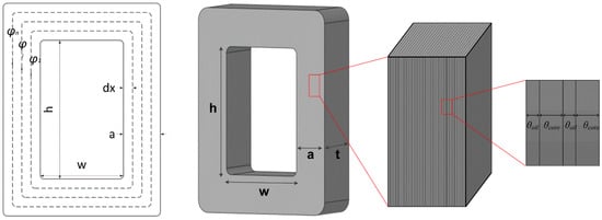
Figure 1.
Structural diagram for core with flat steel sheets and oil layer.
The reluctance of the i-th magnetic segment can be calculated as:
where li is the length of the magnetic path, ε is the material permeability, and Ai is the cross-sectional area of the i-th magnetic path. For the E-E core in use, the following equation can be drawn:
Combining Equations (2)–(5), the following relationship in terms of the reluctance and flux density can be drawn:
where Bi is the flux density of the i-th magnetic segment.
It is explicit from Equations (1) and (6) that the actual core loss varies spatially according to this non-uniform distribution of flux density, i.e. higher core loss allocation occurs in inner locations. To this end, the proposed model scrutinizes the spatial distribution of flux density thus contributes to improving the modeling accuracy of core loss.
2.2. AC Effect and Winding Loss
The ohmic losses in the windings are calculated by:
where J is current density and σ is electric conductivity.
As eddy current effects become more prominent at higher frequency, the effective AC resistance of winding increases as a consequence of the skin and proximity effects. To take eddy current effect into consideration, two well-known analytical models that are applicable to foil and round conductors, respectively, are used in this paper. The classical Dowell’s equation [38] gives the AC resistance of the foil-type winding, assuming that foil conductors occupy the entire height of the core window. The AC factor of the j-th layer (Frn) can be calculated by:
where Δ is the penetration ratio, dfoil the foil thickness, δ the skin depth, and ξ1 and ξ2 the skin and proximity effect respectively.
Dowell’s equation for foil conductors can also be applied on round-type conductors by introducing the porosity factor (η), which is the ratio of the height occupied by conductors to the window height. In addition, in 1990, Ferreira proposed a new solution for round-type wire using the Kelvin–Bessel functions by considering the orthogonality between skin and the proximity effect. However, this formula overlooked the porosity factor. To take Dowell’s porosity coefficient into account and to give a more accurate solution, Bartoli modified Ferreira’s formula and proposed a new model as [39]:
The multilayer configuration of windings are taken into account using Equations (8) and (9), so that the AC resistance for each layer can be calculated more prudently. With the conductor geometry and winding arrangement, the total AC resistance can be derived by accumulating all individual layer resistances:
Dowell’s equation is applicable when the transformer is subject to sinusoidal excitation. In the case of non-sinusoidal excitation, the current can be decomposed into harmonics with Fourier transform, while the loss for each harmonic is calculated by multiplying the harmonic current with the AC resistance under corresponding frequency. The total winding loss can then be determined by summing all of the harmonic losses.
It should be noted that the resistivity of the conductor copper is also temperature-dependent, suggesting that the winding loss is sensitive to the result of thermal modelling. The resistivity of copper can be calculated empirically as:
where φ0 is the resistivity at T0 and τ is the temperature coefficient of copper, which is equal to 0.004041.
3. Thermal-Fluid Simulation
This section goes further to describe the CFD-based thermal-fluid modelling, leveraging the losses that were obtained from the electromagnetic analysis in Section 2.
3.1. Governing Equations
The heat balance for each component of the transformer is expressed as:
Multiple heat transfer processes occurs for the ONAN transformer. The heat is transferred by conduction among the core, winding, and insulation layer. Meanwhile, the heat generated is dissipated from the transformer solid surfaces to the oil via convection. The oil carries the heat that is generated by convection to the tank and finally the heat is dissipated by radiation and convection to the ambient.
The heat conduction, convection, and radiation can be described, respectively, by Fourier’s law, Newton’s law, and Stefan–Boltzmann’s law. The equations are:
where Q is heat generation rate, k is the thermal conductivity, h is the convection coefficient, A is the heat-transfer area, κ is the surface emissivity, δ is the Stefan–Boltzmann’s constant, hr is the equivalent radiation coefficient, and Ts and T∞ is the surface and ambient temperature, respectively.
The mathematical model consists of governing equations simplified from the general expressions for the conservation of mass, momentum, and energy, as follows:
where ρ is the material density, v is velocity, F is body force per unit mass, p is static pressure, μ is dynamic viscosity, Cp is specific heat capacity, and λ is heat conductivity.
3.2. Boundary Conditions
No-slip boundary condition is defined at the fluid-solid interface. The temperature and heat transfer are continuous at all interfaces. In the meantime, equal momentum and heat transfer between liquid-gas interfaces and free surface are defined.
Convection heat transfer occurs when the fluid flows along the solid surface between the fluid and the solid. The convection heat transfer coefficient can be calculated with:
where Nu is the Nusselt number, kf is the thermal conductivity of fluid, and L is the characteristic length.
The Nusselt number for vertical and horizontal enclosures and for vertical flat plates are calculated as:
where Ra, Gr, and Pr are the Rayleigh, Grashof, and Prandtl numbers of the fluid, respectively, which are defined as:
where g is acceleration of gravity, λ is the fluid volumetric expansion coefficient, and ΔT is the temperature difference between surface and fluid.
3.3. Determination of Thermal Parameters
The thermal-fluid system can be solved with Equations (14)–(17), where the parameters are temperature-dependent. Therefore, these parameters should be included into the simulation in the form of parametric equations. The dependence of thermal parameters of the core and winding materials to the temperature is considered by incorporating the equations in Table 1. The temperature-dependent physical properties of mineral oil can be calculated by equations in Table 2.

Table 1.
Thermal Parameters of Core and Winding Materials.
Table 2.
Thermal Parameters of Mineral Oil.
The core is assumed to be a solid compound consisting of flat steel sheets interspersed with oil. The schematic illustration of the core structure is shown in Figure 1, where θoil and θcore represents the layer thickness of oil layer and steel sheet, respectively. The conduction process is assumed to be orthotropic with equivalent normal thermal conductivity (keq,n) and transversal thermal conductivity (keq,t), which can be calculated as:
The equivalent density (ρeq) and specific heat (Cp,eq) of the core are calculated with:
where S is the stacking factor.
3.4. Coupled and Semi-numerical Framework
The solution begins with an analytical electromagnetic model for the determination of core loss and winding loss. Leveraging the obtained losses, the thermal-fluid simulation is performed using Ansys Fluent for steady-state analysis. The computing domain is discretized and the total number of grids is determined by performing the grid independence test to reduce the computational effort while keeping adequate accuracy [40]. The temperature dependence of material properties shown in Table 1 and Table 2 are taken into account with the user-defined function (UDF). The SIMPLE algorithm was employed to handle the velocity-pressure coupling in the flow field equations. The pressure discretization is performed with the body force weighted scheme. The second-order upwind scheme was applied for the space derivatives of advection terms in all transport equations.
The analytical model and the CFD model are combined in a sequential and iterative framework, as shown in Figure 2, to address the intrinsic coupling between electromagnetic and thermal behaviors. The overall convergence is achieved when the changes of losses and temperature during two adjacent iterations are no more than their respective thresholds. Based on the proposed coupled, semi-numerical framework, the steady-state losses, oil flow pattern, and temperature distribution can be obtained.
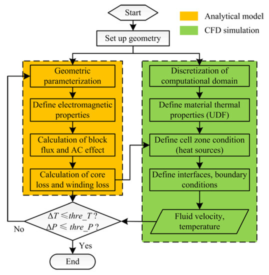
Figure 2.
Overall framework of the coupled and semi-numerical method.
4. Experiment
4.1. Prototypes and Experimental Setup
Two ONAN single-phase transformers with different designs are investigated. The operating power is 5 kVA, while the LV (primary) and HV (high-voltage) (secondary) voltages are 500 V and 5 kV, respectively. The other major system specifications are summarized in Table 3. Both two prototypes use the P-S design and they are placed in the oil tank with the dimension of 200 mm × 200 mm × 200 mm. An experimental setup consisting of ONAN prototypes, programmable power source, load bank, monitoring units, data collection and storage units are built for testing, as shown in Figure 3. Specifically, the LV side is supplied with 1 kHz voltage by using Pacific AC source with programmable controller and output impedance, while the HV side is regulated with programmable load bank to achieve the expected power. The current and voltage are continuously monitored with DSOS054A High-Definition Oscilloscope during the tests and load experiments. The real-time power is measured by aWT3000E Precision Power Analyzer.
Table 3.
Specifications of transformer prototypes.
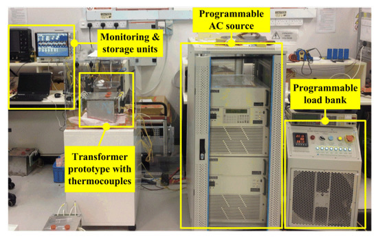
Figure 3.
Experimental setup for validation.
4.2. Loss Measurement
The core loss is measured by supplying the LV side with the expected voltage and opening the HV side. The open circuit setup allows for full core excitation but extremely low currents in the windings. Therefore, winding losses are negligible and the core loss is approximately equal to the observed total active power, which can be obtained by calculating the mean of the product of current and voltage. The winding loss can be measured by feeding the HV side with sinusoidal voltage while leaving the LV side short circuited. The voltage is stepped up gradually until the current reaches the expected value (1 A in HV side). The flux density in core during the short-circuit test is negligible as the HV side is excited with minimal voltage. In this case, the core loss is ignorable and the observed total loss is the HV winding loss.
4.3. Temperature Measurement
Direct temperature measurement, although quite costly, shows a high accuracy thus has been widely used for model validation. A certain number of temperature measurement points have been selected for each prototype, as shown in Figure 4, to collect the reference temperature and compare with the predicted values. J-type thermocouples are inserted to the illustrated positions during the manufacturing process. The accuracy of temperature sensing is ±2.2 °C within an operating range from 0 °C to 760 °C. Both prototypes are operated with 5 kVA to obtain the transient temperature response. A laptop that was equipped with BV0006B Data Acquisition Control & Automation software is connected to the 34972A Data Acquisition Switch Unit to acquire the temperature. Load experiments are terminated once the temperature variations are less than 1 °C per hour, which serves as the steady state criterion in this study.
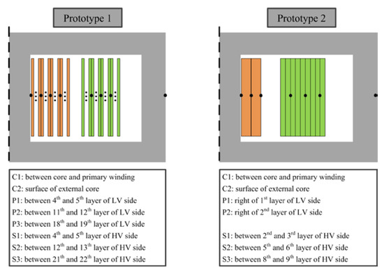
Figure 4.
Thermocouple locations (Note: the figure does not represent the real geometry of transformer design; it is a diagram to identify the relative locations of temperature measurement points).
5. Validation
5.1. Validation of Losses Determination
The core losses and winding losses determined by the proposed semi-numerical model and the full numerical model in comparison with the real measurements are shown in Table 4 and Table 5, respectively. It is shown that the modelling results are in reasonable agreement with the measured values, suggesting that the proposed method can simulate the electro-magnetic behaviours of HF transformers well. Meanwhile, the semi-numerical model provides similar accuracy when compared with the full numerical model. Hence, it is validated that the reduction of computing cost does not compromise the modelling accuracy.
Table 4.
Comparison of modeled core losses and measurements.
Table 5.
Comparison of modeled winding losses and measurements.
The proposed method also scrutinizes the AC effects in each winding layer. Due to the difficulty of measuring layer losses, the proposed semi-numerical model is compared with the FEM-CFD method for validation. The FEM-CFD approach is a full numerical method that uses the same structure as in Figure 2 while the analytical part is replaced by 3D steady-state FEM with Ansys Maxwell. The comparison results of layer losses are shown in Figure 5. It is shown that the layer losses calculated by the semi-numerical method are benchmarked with FEM results. The mean relative deviations of two methods are 8.9% and 4.9% for prototypes 1 and 2, respectively. A scrutiny of the deviation suggests that the proposed method underestimates the losses slightly as compared to the full numerical method. This is due to the existence of edge effect, which is not considered by the analytical model.
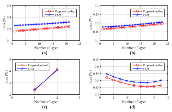
Figure 5.
Losses of different winding layers: (a) low-voltage (LV) winding of prototype 1; (b) HV winding of prototype 1; (c) LV winding of prototype 2; and, (d) HV winding of prototype 2.
The deviation of two methods can be better explained by analysing the current density and magnetic field distribution on conductors and core window, as shown in Figure 6. It is shown that the proximity effect is quite obvious at the middle part of winding in the vertical direction, and tends to be severe at the boundary between the LV and HV windings. The proposed semi-numerical model shows to well describe the proximity effect. In contrast, the current density distribution is highly non-uniform at the upper and bottom corner of LV winding. This is attributed to the edge effect that is caused by the orthogonal component of magnetic field around the winding edge, as shown in the upper zoom-in figure of Figure 6a,b. While the proposed method well considers the skin and proximity effect, it overlooks the edge effect, so that its underestimation of AC losses is within expectation.
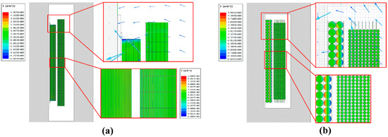
Figure 6.
Magnetic field and current density distribution from finite element modelling-computational fluid dynamics (FEM-CFD) approach: (a) prototype 1; and, (b) prototype 2.
The edge effect observed in prototype 2 is not as strong as in the case of prototype 1. This is because prototype 2 has a larger filling factor (the ratio of winding height to the core window height), which prohibits the tangential component of magnetic field at the edge regions. Therefore, a higher filling factor is always favourable to alleviate the extra losses that are caused by the edge effect. The milder edge effect also coincides with the aforementioned result that the deviation of two methods is smaller for the case of prototype 2. It should be mentioned that the skin effect is not obvious for both the two prototypes, as the skin depth under the applied frequency is at the same level with the characteristic length of conductors.
5.2. Validation of Temperature Prediction
In seeking to validate the temperature prediction, the proposed method is validated by comparing with both the full numerical model and experimental results. Three simulations have been performed for each prototype to validate the creditability of the simulation results. The simulation result of temperature distribution is shown in Figure 7. It is explicit that a temperature gradient exists along the vertical direction of transformer active components and oil. This is because the hot oil keeps rising to the upper section of tank that is driven by the buoyancy force. The central core and inner winding layers show higher temperature due to significant losses and the poor heat dissipation condition.
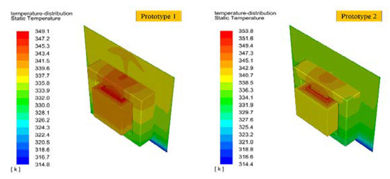
Figure 7.
Temperature distribution in transformer active components and oil for the two investigated prototypes.
The predicted temperatures at measurement points are compared with experimental data to evaluate the prediction accuracy. The temperatures obtained from the semi-numerical model and full-numerical model in comparison with measurements are shown in Figure 8. The relative deviations between simulation and measurement calculated by (Tsimu − Tmeas)/Tmeas are summarized in Table 6. It is shown that the predicted temperature by both the two models is benchmarked with the measurement data with reasonable accuracy. The prediction errors for the central core and windings are well confined to approximately 10%. In contrast, the proposed semi-numerical model overestimates the temperature of the external core, as seen from the relatively large prediction errors exceeding 10%. One possible explanation is that the model for thermal conductivity calculation in Figure 1 may be deviated from real prototypes, due to the uncertainties in the manufacturing process. The proposed method is experimental verified with sufficient accuracy in temperature prediction, especially when considering the unavoidable mismatch between designed geometry and real prototypes. Moreover, the proposed semi-numerical model shows to give similar accuracy when compared with the computationally expensive full-numerical model, suggesting that the proposed technique lowers the computing cost without compromising the modelling accuracy.
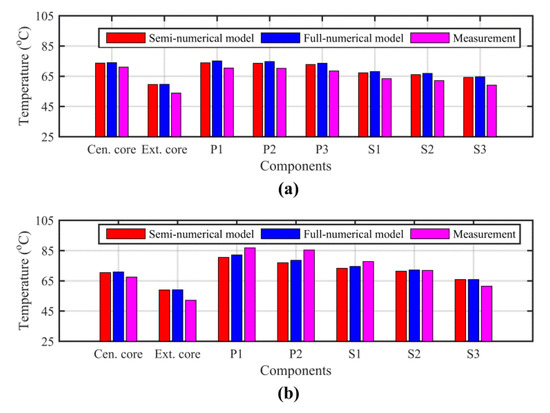
Figure 8.
Comparison between simulated and measured temperature at different locations: (a) Prototype 1 and (b) Prototype 2.
Table 6.
Relative deviations between predicted and measured temperatures.
5.3. Discussion
It should be noted the proposed semi-numerical model is a general one that is able to provide accurate prediction of losses and the temperature response of transformer. This section goes further to discuss the extendibility of the proposed model by analysing each sub-model, i.e. core loss model, winding loss model, and thermal-fluid model. The refined core loss model can be easily extended to any magnetic material, structure, and frequency by scrutinizing the special distribution of the flux density. The layer-based winding loss model takes the skin effect, proximity effect, and radial geometric inhomogeneity into account to better describe the resistive feature. From theoretical point of view, the proposed model is applicable at lower frequency, such as 50/60 Hz, since the AC effects are not substantial in this case and they are generally easier for modeling. In contrast, albeit aiming to improve the modeling of AC effects, the proposed model is subject to an accuracy declination at higher frequency, since secondary AC effects, such as the edge effect have been overlooked. This has already been shown in Figure 5 and Figure 6, where explicitly an underestimate of winding losses has been observed. With respect to the thermal-hydraulic model, the numerical model leveraging CFD is performed to obtain the detailed flow characteristic, thermal path, and temperature distribution. This sub-model stands for the state of art for modeling of the thermal behavior of transformer and enjoys a good extendibility in terms of the selection of material, geometry, operating conditions, and cooling medium, provided that the losses can be determined with reasonable credibility.
6. Conclusions
This paper proposes a coupled, semi-numerical model for the thermal analysis of MF ONAN transformers. An analytical model has been exploited based on spatial distribution of flux density and AC factor to calculate the core and winding losses, while the CFD simulation has been used for thermal-fluid analysis. The electromagnetic and thermal-fluid behaviours are solved iteratively in a close-loop manner by leveraging the analytical and CFD model, respectively. Lab-scale experiments have been carried out on two prototypes with different designs. Results show that the AC effects, losses, and temperature rise can be well predicted by the proposed method. The predicted temperature is benchmarked with experimental data with a reasonable accuracy. The proposed semi-numerical model is technically feasible and experimentally validated, so that it is promising to be used for transformer design optimization and operating performance prediction. It is also preferable when compared to the coupled full numerical approach due to the better trade-off between modelling accuracy and computing cost.
Author Contributions
Conceptualization, H.T. and A.T.; Investigation, H.T. and Z.W.; Methodology, H.T.; Project administration, S.V.; Resources, A.T. and P.K.; Validation, H.T., Z.W. and M.T.; Writing—original draft, H.T.; Writing—review & editing, Z.W. and S.V.
Funding
This research received no external funding.
Acknowledgments
Authors would like to extend their gratitude to Vestas Wind System A/S, Denmark and Energy Research Institute @ NTU, Nanyang Technological University, for accommodating above research work.
Conflicts of Interest
The authors declare no conflict of interest.
References
- Pierce, L.W. Predicting liquid filled transformer loading capability. In Proceedings of the [1992] Record of Conference Papers Industry Applications Society 39th Annual Petroleum and Chemical Industry Conference, San Antonio, TX, USA, 28 September 1992; pp. 197–207. [Google Scholar]
- Cheng, L.; Yu, T.; Wang, G.; Yang, B.; Zhou, L. Hot spot temperature and grey target theory-based dynamic modelling for reliability assessment of transformer oil-paper insulation systems: A practical case study. Energies 2018, 11, 249. [Google Scholar] [CrossRef]
- Hu, E.; Yang, L.; Liao, R.J.; Liu, Y.; Yuan, Y. Effect of an electric field on copper sulphide deposition in oil-impregnated power transformers. IET Electr. Power Appl. 2016, 10, 155–160. [Google Scholar] [CrossRef]
- Leibl, M.; Ortiz, G.; Kolar, J.W. Design and experimental analysis of a medium-frequency transformer for solid-state transformer applications. IEEE J. Emerg. Sel. Top. Power Electron. 2017, 5, 110–123. [Google Scholar] [CrossRef]
- Faiz, J.; Ghazizadeh, M.; Oraee, H. Derating of transformers under non-linear load current and non-sinusoidal voltage—An overview. IET Electr. Power Appl. 2015, 9, 486–495. [Google Scholar] [CrossRef]
- Zhang, L.; Zhang, W.; Liu, J.; Zhao, T.; Zou, L.; Wang, X. A New Prediction Model for Transformer Winding Hotspot Temperature Fluctuation Based on Fuzzy Information Granulation and an Optimized Wavelet Neural Network. Energies 2017, 10, 1998. [Google Scholar] [CrossRef]
- Wei, Z.; Zhao, J.; Xiong, R.; Dong, G.; Pou, J.; Tseng, K.J. Online Estimation of Power Capacity with Noise Effect Attenuation for Lithium-Ion Battery. IEEE Trans. Ind. Electron. 2018. [Google Scholar] [CrossRef]
- Wei, Z.; Zou, C.; Leng, F.; Soong, B.H.; Tseng, K.-J. Online model identification and state-of-charge estimate for lithium-ion battery with a recursive total least squares-based observer. IEEE Trans. Ind. Electron. 2018, 65, 1336–1346. [Google Scholar] [CrossRef]
- Wei, Z.; Lim, T.M.; Skyllas-Kazacos, M.; Wai, N.; Tseng, K.J. Online state of charge and model parameter co-estimation based on a novel multi-timescale estimator for vanadium redox flow battery. Appl. Energy 2016, 172, 169–179. [Google Scholar] [CrossRef]
- Chen, W.; Ma, J.; Huang, X.; Fang, Y. Predicting iron losses in laminated steel with given non-sinusoidal waveforms of flux density. Energies 2015, 8, 13726–13740. [Google Scholar] [CrossRef]
- Tria, L.A.R.; Zhang, D.; Fletcher, J.E. Planar PCB transformer model for circuit simulation. IEEE Trans. Magn. 2016, 52, 1–4. [Google Scholar] [CrossRef]
- Ghazizadeh, M.; Faiz, J.; Oraee, H. Derating of distribution transformers under non-linear loads using a combined analytical-finite elements approach. IET Electr. Power Appl. 2016, 10, 779–787. [Google Scholar] [CrossRef]
- International Electrotechnical Commission. IEC 60076-7 Power Transformers Part 7: Loading Guide for Oil-Immersed Power Transformers; IEC: Geneva, Switzerland, 2005. [Google Scholar]
- IEEE-SA Standards Board. IEEE Guide for Loading Mineral-Oilimmersed Transformers; IEEE Std C57.91-1995; IEEE: Hoboken, NJ, USA, 1996; pp. 1–112. [Google Scholar]
- Degefa, M.; Millar, R.; Lehtonen, M.; Hyvonen, P. Dynamic thermal modeling of mv/lv prefabricated substations. IEEE Trans. Power Deliv. 2014, 29, 786–793. [Google Scholar] [CrossRef]
- Radakovic, Z.; Jacic, D.; Lukic, J.; Milosavljevic, S. Loading of transformers in conditions of controlled cooling system. Int. Trans. Electr. Energy Syst. 2014, 24, 203–214. [Google Scholar] [CrossRef]
- Feng, D.; Wang, Z.; Jarman, P. Evaluation of Power Transformers’ Effective Hot-Spot Factors by Thermal Modeling of Scrapped Units. IEEE Trans. Power Deliv. 2014, 29, 2077–2085. [Google Scholar] [CrossRef]
- Roslan, M.; Azis, N.; Kadir, M.; Jasni, J.; Ibrahim, Z.; Ahmad, A. A Simplified Top-Oil Temperature Model for Transformers Based on the Pathway of Energy Transfer Concept and the Thermal-Electrical Analogy. Energies 2017, 10, 1843. [Google Scholar] [CrossRef]
- Cui, Y.; Ma, H.; Saha, T.; Ekanayake, C.; Martin, D. Moisture-dependent thermal modelling of power transformer. IEEE Trans. Power Deliv. 2016, 31, 2140–2150. [Google Scholar] [CrossRef]
- Zhang, J.; Li, X. Oil cooling for disk-type transformer windings-part 1: Theory and model development. IEEE Trans. Power Deliv. 2006, 21, 1318–1325. [Google Scholar] [CrossRef]
- Djamali, M.; Tenbohlen, S. Malfunction detection of the cooling system in air-forced power transformers using online thermal monitoring. IEEE Trans. Power Deliv. 2017, 32, 1058–1067. [Google Scholar] [CrossRef]
- Weinlader, A.; Wu, W.; Tenbohlen, S.; Wang, Z. Prediction of the oil flow distribution in oil-immersed transformer windings by network modelling and computational fluid dynamics. IET Electr. Power Appl. 2012, 6, 82–90. [Google Scholar] [CrossRef]
- Ji, D.; Wei, Z.; Mazzoni, S.; Mengarelli, M.; Rajoo, S.; Zhao, J.; Pou, J.; Romagnoli, A. Thermoelectric generation for waste heat recovery: Application of a system level design optimization approach via Taguchi method. Energy Convers. Manag. 2018, 172, 507–516. [Google Scholar] [CrossRef]
- Ji, D.; Tseng, K.J.; Wei, Z.; Zheng, Y.; Romagnoli, A. A Simulation Study on a Thermoelectric Generator for Waste Heat Recovery from a Marine Engine. J. Electron. Mater. 2017, 46, 2908–2914. [Google Scholar] [CrossRef]
- Wei, Z.; Zhao, J.; Ji, D.; Tseng, K.J. A multi-timescale estimator for battery state of charge and capacity dual estimation based on an online identified model. Appl. Energy 2017, 204, 1264–1274. [Google Scholar] [CrossRef]
- Kim, Y.J.; Jeong, M.; Park, Y.G.; Ha, M.Y. A numerical study of the effect of a hybrid cooling system on the cooling performance of a large power transformer. Appl. Therm. Eng. 2018, 136, 275–286. [Google Scholar] [CrossRef]
- Fernández, I.; Delgado, F.; Ortiz, F.; Ortiz, A.; Fernández, C.; Renedo, C.J.; Santisteban, A. Thermal degradation assessment of Kraft paper in power transformers insulated with natural esters. Appl. Therm. Eng. 2016, 104, 129–138. [Google Scholar] [CrossRef]
- Huang, P.; Mao, C.; Wang, D. Electric field simulations and analysis for high voltage high power medium frequency transformer. Energies 2017, 10, 371. [Google Scholar] [CrossRef]
- Tenbohlen, S.; Schmidt, N.; Breuer, C.; Khandan, S.; Lebreton, R. Investigation of Thermal Behavior of an Oil-Directed Cooled Transformer Winding. IEEE Trans. Power Deliv. 2018, 33, 1091–1098. [Google Scholar] [CrossRef]
- Tomczuk, B.Z.; Koteras, D.; Waindok, A. Electromagnetic and temperature 3-D fields for the modular transformers heating under high-frequency operation. IEEE Trans. Magn. 2014, 50, 317–320. [Google Scholar] [CrossRef]
- Gong, R.; Ruan, J.; Chen, J.; Quan, Y.; Wang, J.; Duan, C. Analysis and Experiment of Hot-Spot Temperature Rise of 110 kV Three-Phase Three-Limb Transformer. Energies 2017, 10, 1079. [Google Scholar] [CrossRef]
- Da Silva, J.R.; Bastos, J.P. Online Evaluation of Power Transformer Temperatures Using Magnetic and Thermodynamics Numerical Modeling. IEEE Trans. Magn. 2017, 53, 1–4. [Google Scholar] [CrossRef]
- Gong, R.; Ruan, J.; Chen, J.; Quan, Y.; Wang, J.; Jin, S. A 3-D Coupled Magneto-Fluid-Thermal Analysis of a 220 kV Three-Phase Three-Limb Transformer under DC Bias. Energies 2017, 10, 422. [Google Scholar] [CrossRef]
- Liu, C.; Ruan, J.; Wen, W.; Gong, R.; Liao, C. Temperature rise of a dry-type transformer with quasi-3D coupled-field method. IET Electr. Power Appl. 2016, 10, 598–603. [Google Scholar] [CrossRef]
- Liu, G.; Zheng, Z.; Yuan, D.; Li, L.; Wu, W. Simulation of Fluid-Thermal Field in Oil-Immersed Transformer Winding Based on Dimensionless Least-Squares and Upwind Finite Element Method. Energies 2018, 11, 2357. [Google Scholar] [CrossRef]
- Steinmetz, C.P. On the law of hysteresis. Trans. Am. Inst. Electr. Eng. 1892, 9, 1–64. [Google Scholar] [CrossRef]
- Venkatachalam, K.; Sullivan, C.R.; Abdallah, T.; Tacca, H. Accurate prediction of ferrite core loss with nonsinusoidal waveforms using only Steinmetz parameters. In Proceedings of the 2002 IEEE Workshop on Computers in Power Electronics, Mayaguez, PR, USA, 3–4 June 2002; pp. 36–41. [Google Scholar]
- Dowell, P. Effects of eddy currents in transformer windings. Proc. Inst. Electr. Eng. 1966, 113, 1387–1394. [Google Scholar] [CrossRef]
- Reatti, A.; Kazimierczuk, M.K. Comparison of various methods for calculating the AC resistance of inductors. IEEE Trans. Magn. 2002, 38, 1512–1518. [Google Scholar] [CrossRef]
- Wei, Z.; Li, X.; Xu, L.; Tan, C. Optimization of Operating Parameters for Low NOx Emission in High-Temperature Air Combustion. Energy Fuels 2012, 26, 2821–2829. [Google Scholar] [CrossRef]
© 2019 by the authors. Licensee MDPI, Basel, Switzerland. This article is an open access article distributed under the terms and conditions of the Creative Commons Attribution (CC BY) license (http://creativecommons.org/licenses/by/4.0/).