A Coupled, Semi-Numerical Model for Thermal Analysis of Medium Frequency Transformer

Abstract
:1. Introduction
2. Electromagnetic Modeling
2.1. Core Loss
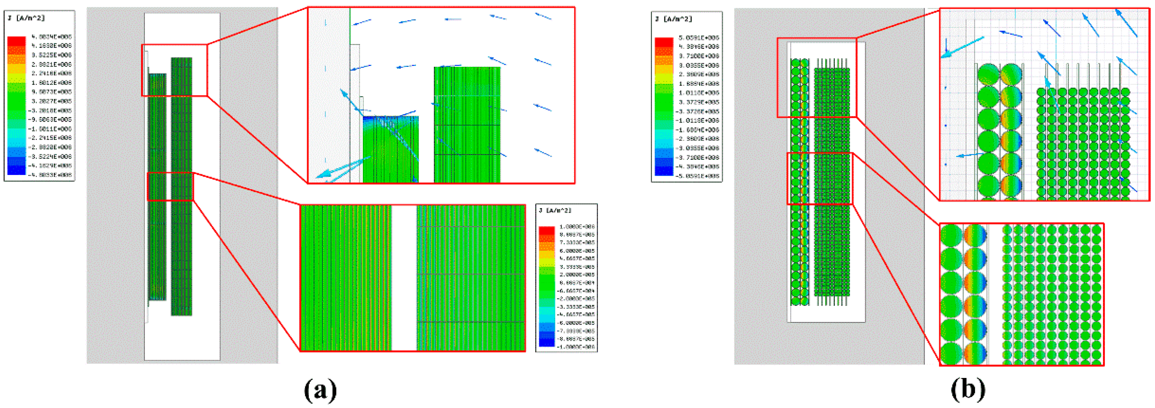
2.2. AC Effect and Winding Loss
3. Thermal-Fluid Simulation
3.1. Governing Equations
3.2. Boundary Conditions
3.3. Determination of Thermal Parameters
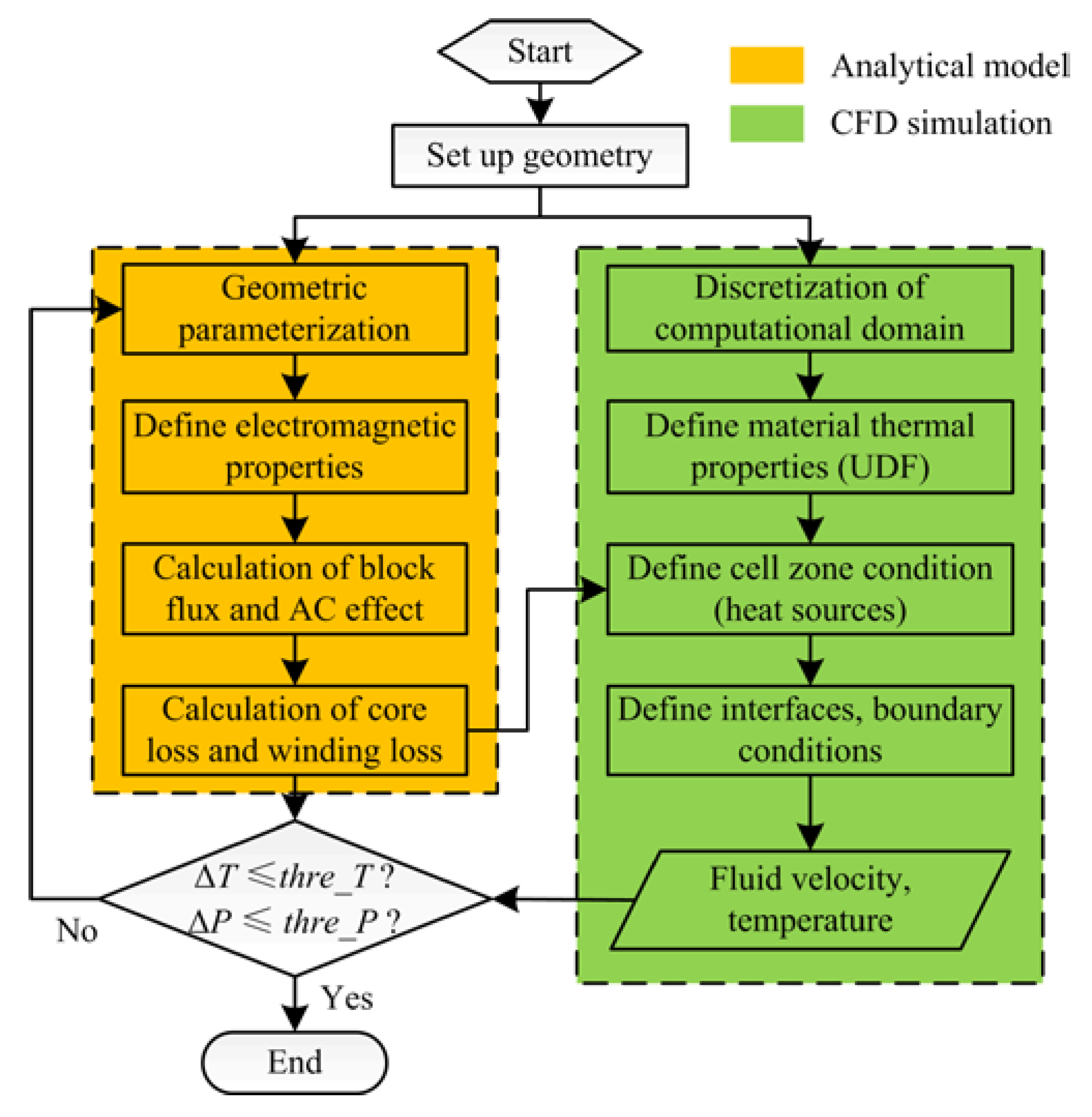
3.4. Coupled and Semi-numerical Framework
4. Experiment
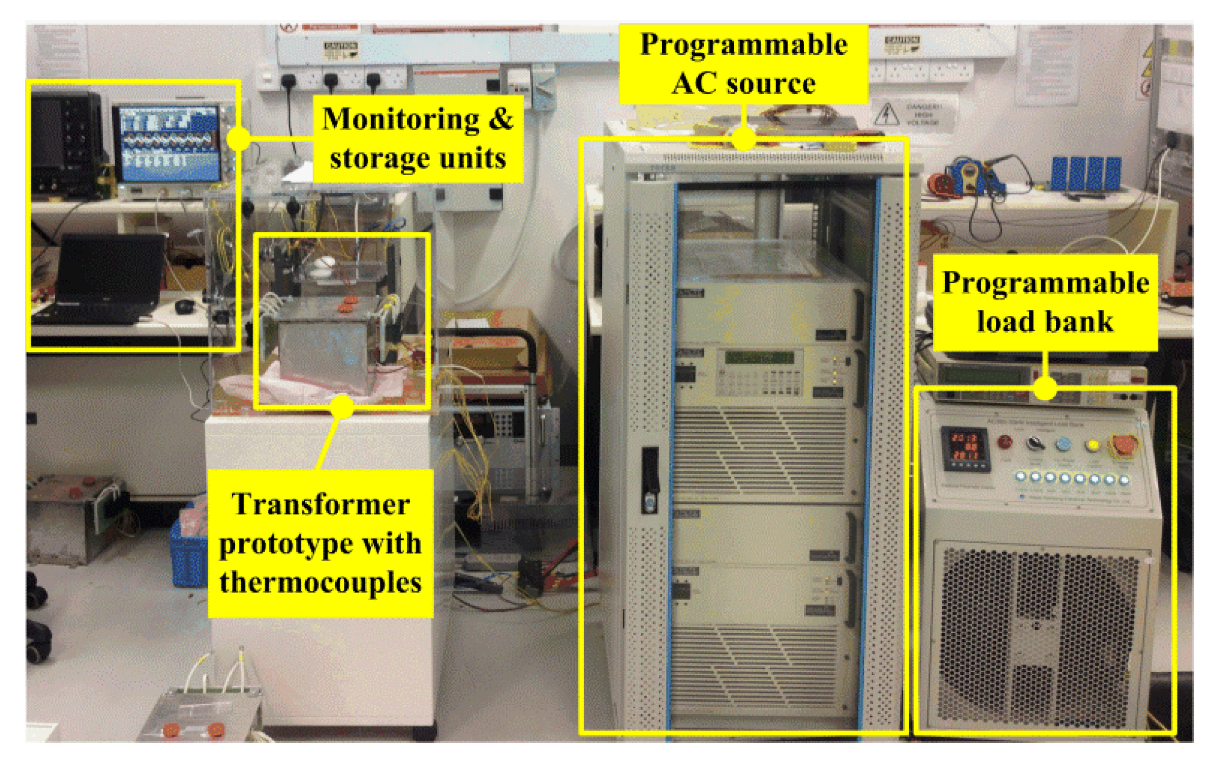
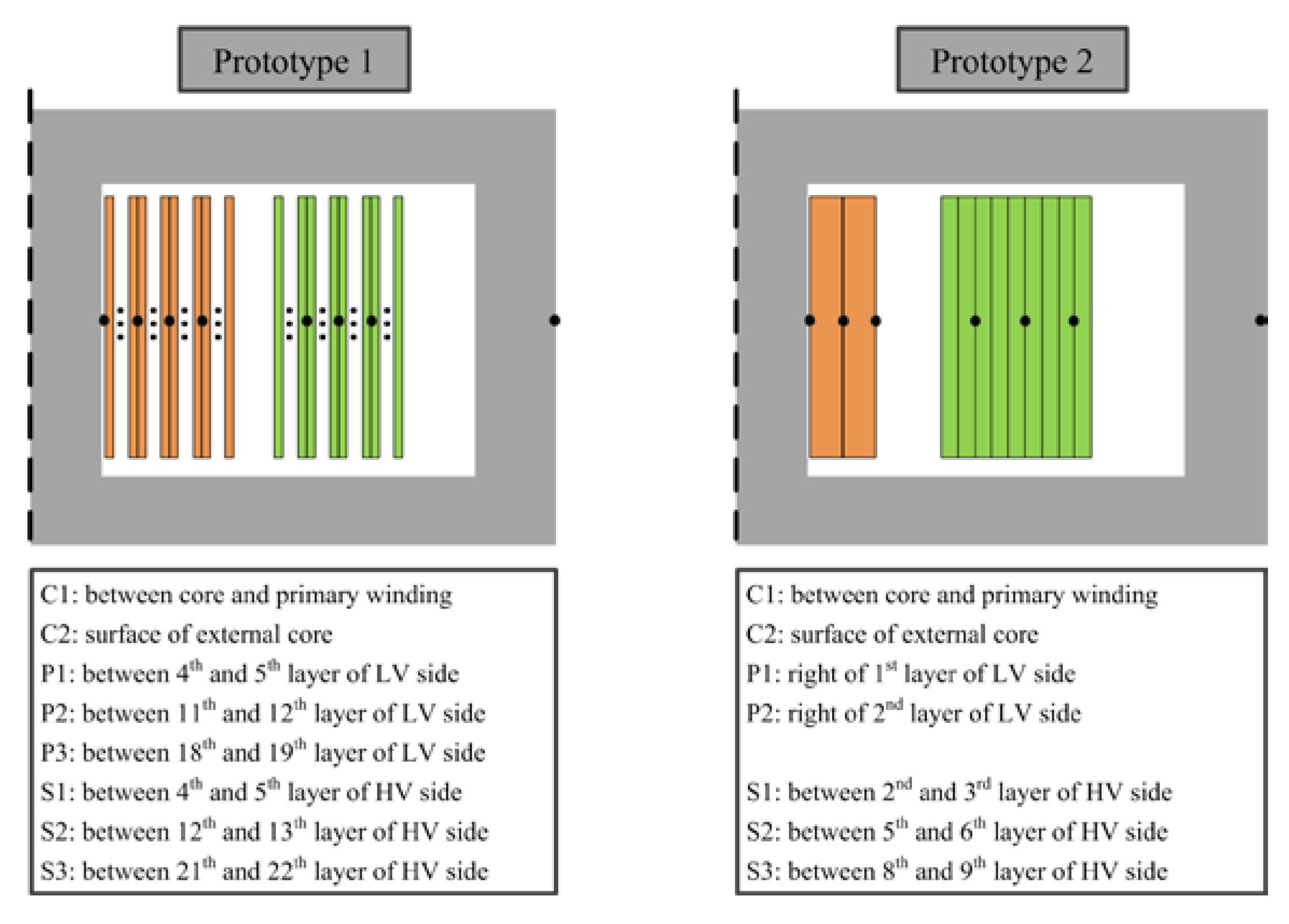
4.1. Prototypes and Experimental Setup
4.2. Loss Measurement
4.3. Temperature Measurement
5. Validation
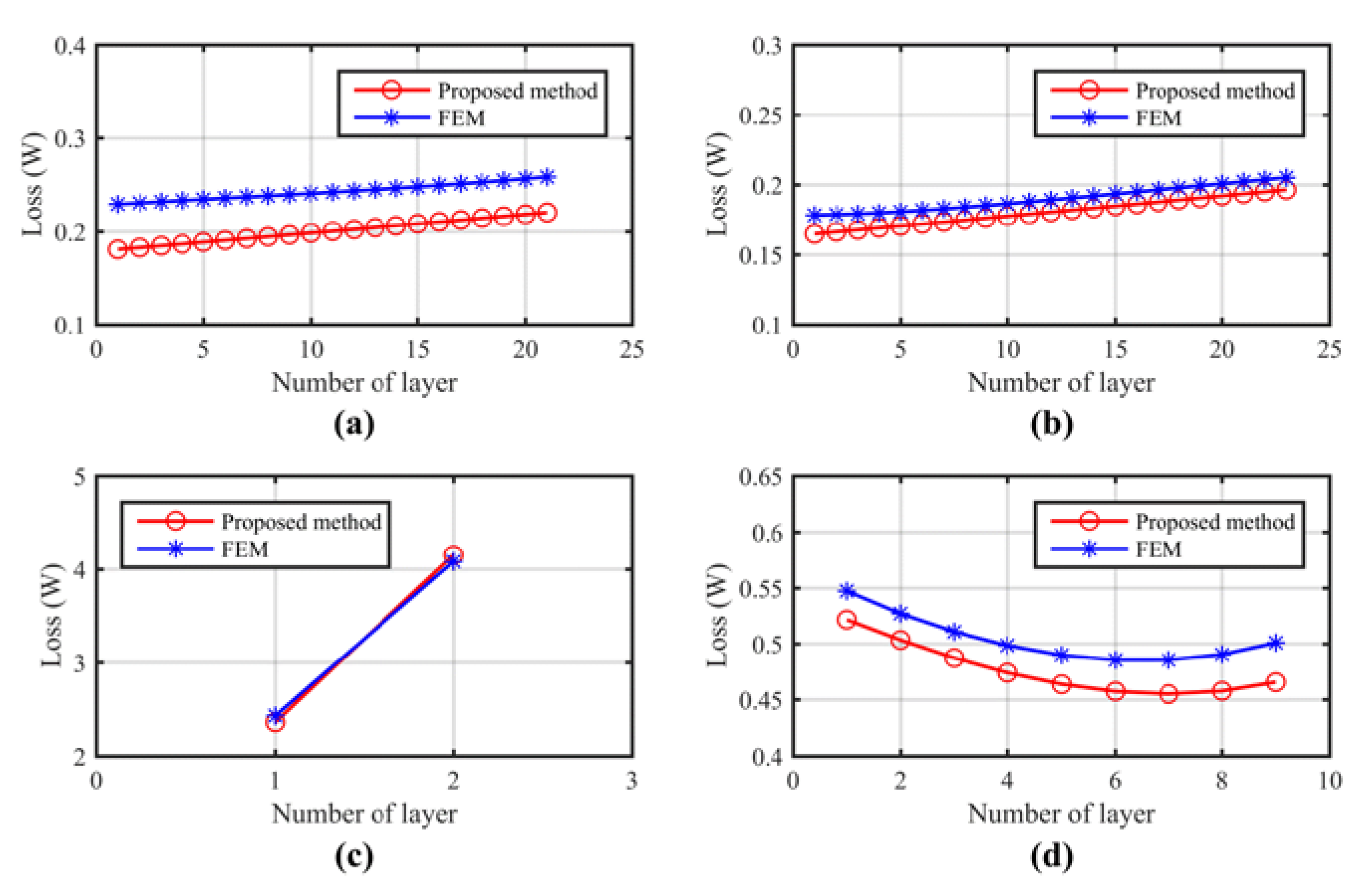
5.1. Validation of Losses Determination
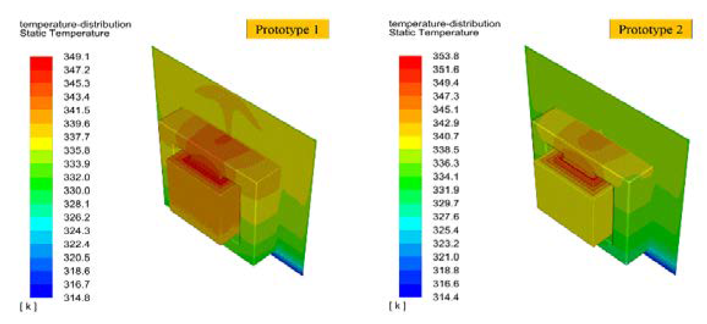
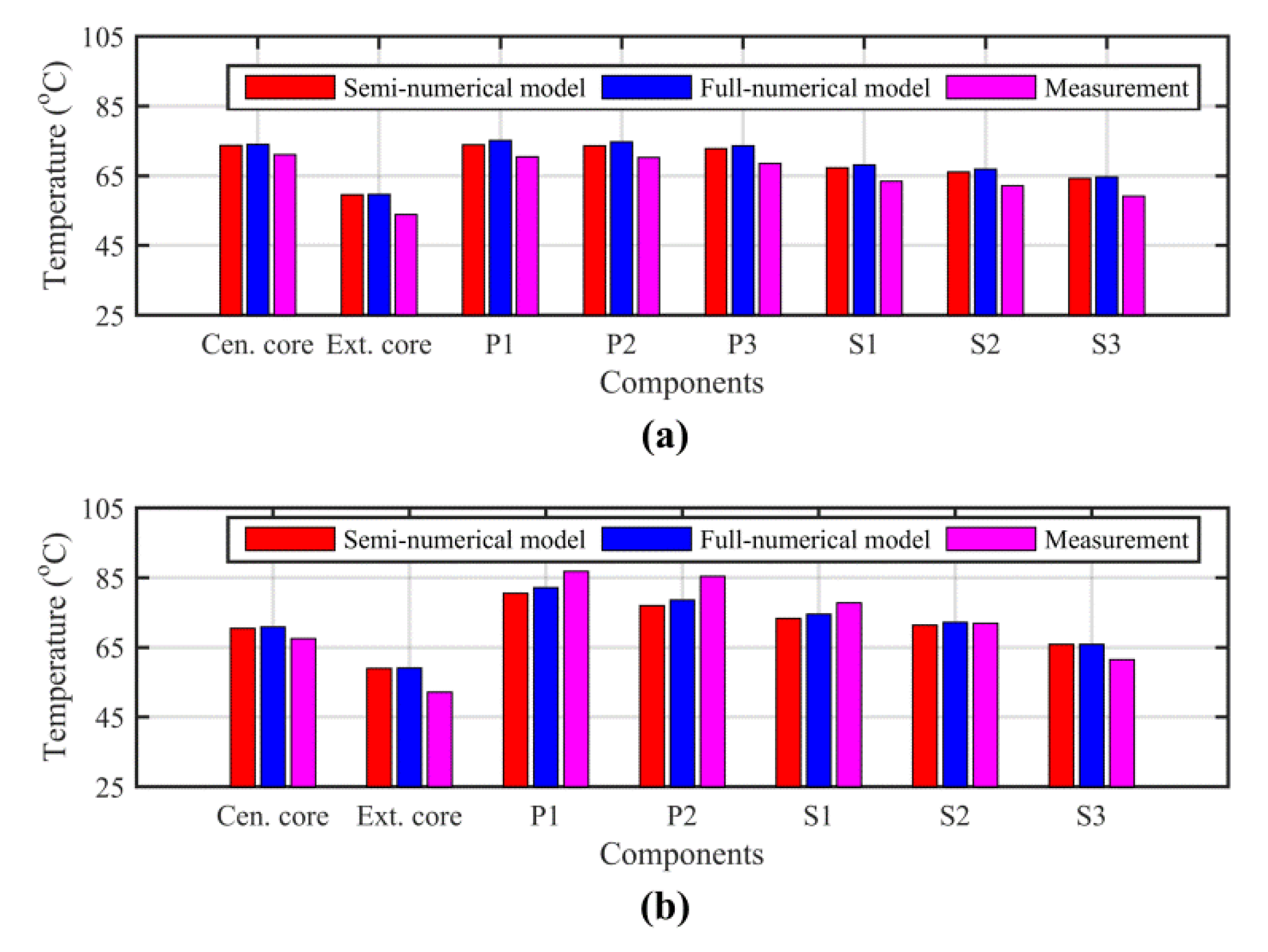
5.2. Validation of Temperature Prediction
5.3. Discussion
6. Conclusions
Author Contributions
Funding
Acknowledgments
Conflicts of Interest
References
- Pierce, L.W. Predicting liquid filled transformer loading capability. In Proceedings of the [1992] Record of Conference Papers Industry Applications Society 39th Annual Petroleum and Chemical Industry Conference, San Antonio, TX, USA, 28 September 1992; pp. 197–207. [Google Scholar]
- Cheng, L.; Yu, T.; Wang, G.; Yang, B.; Zhou, L. Hot spot temperature and grey target theory-based dynamic modelling for reliability assessment of transformer oil-paper insulation systems: A practical case study. Energies 2018, 11, 249. [Google Scholar] [CrossRef]
- Hu, E.; Yang, L.; Liao, R.J.; Liu, Y.; Yuan, Y. Effect of an electric field on copper sulphide deposition in oil-impregnated power transformers. IET Electr. Power Appl. 2016, 10, 155–160. [Google Scholar] [CrossRef]
- Leibl, M.; Ortiz, G.; Kolar, J.W. Design and experimental analysis of a medium-frequency transformer for solid-state transformer applications. IEEE J. Emerg. Sel. Top. Power Electron. 2017, 5, 110–123. [Google Scholar] [CrossRef]
- Faiz, J.; Ghazizadeh, M.; Oraee, H. Derating of transformers under non-linear load current and non-sinusoidal voltage—An overview. IET Electr. Power Appl. 2015, 9, 486–495. [Google Scholar] [CrossRef]
- Zhang, L.; Zhang, W.; Liu, J.; Zhao, T.; Zou, L.; Wang, X. A New Prediction Model for Transformer Winding Hotspot Temperature Fluctuation Based on Fuzzy Information Granulation and an Optimized Wavelet Neural Network. Energies 2017, 10, 1998. [Google Scholar] [CrossRef]
- Wei, Z.; Zhao, J.; Xiong, R.; Dong, G.; Pou, J.; Tseng, K.J. Online Estimation of Power Capacity with Noise Effect Attenuation for Lithium-Ion Battery. IEEE Trans. Ind. Electron. 2018. [Google Scholar] [CrossRef]
- Wei, Z.; Zou, C.; Leng, F.; Soong, B.H.; Tseng, K.-J. Online model identification and state-of-charge estimate for lithium-ion battery with a recursive total least squares-based observer. IEEE Trans. Ind. Electron. 2018, 65, 1336–1346. [Google Scholar] [CrossRef]
- Wei, Z.; Lim, T.M.; Skyllas-Kazacos, M.; Wai, N.; Tseng, K.J. Online state of charge and model parameter co-estimation based on a novel multi-timescale estimator for vanadium redox flow battery. Appl. Energy 2016, 172, 169–179. [Google Scholar] [CrossRef]
- Chen, W.; Ma, J.; Huang, X.; Fang, Y. Predicting iron losses in laminated steel with given non-sinusoidal waveforms of flux density. Energies 2015, 8, 13726–13740. [Google Scholar] [CrossRef]
- Tria, L.A.R.; Zhang, D.; Fletcher, J.E. Planar PCB transformer model for circuit simulation. IEEE Trans. Magn. 2016, 52, 1–4. [Google Scholar] [CrossRef]
- Ghazizadeh, M.; Faiz, J.; Oraee, H. Derating of distribution transformers under non-linear loads using a combined analytical-finite elements approach. IET Electr. Power Appl. 2016, 10, 779–787. [Google Scholar] [CrossRef]
- International Electrotechnical Commission. IEC 60076-7 Power Transformers Part 7: Loading Guide for Oil-Immersed Power Transformers; IEC: Geneva, Switzerland, 2005. [Google Scholar]
- IEEE-SA Standards Board. IEEE Guide for Loading Mineral-Oilimmersed Transformers; IEEE Std C57.91-1995; IEEE: Hoboken, NJ, USA, 1996; pp. 1–112. [Google Scholar]
- Degefa, M.; Millar, R.; Lehtonen, M.; Hyvonen, P. Dynamic thermal modeling of mv/lv prefabricated substations. IEEE Trans. Power Deliv. 2014, 29, 786–793. [Google Scholar] [CrossRef]
- Radakovic, Z.; Jacic, D.; Lukic, J.; Milosavljevic, S. Loading of transformers in conditions of controlled cooling system. Int. Trans. Electr. Energy Syst. 2014, 24, 203–214. [Google Scholar] [CrossRef]
- Feng, D.; Wang, Z.; Jarman, P. Evaluation of Power Transformers’ Effective Hot-Spot Factors by Thermal Modeling of Scrapped Units. IEEE Trans. Power Deliv. 2014, 29, 2077–2085. [Google Scholar] [CrossRef]
- Roslan, M.; Azis, N.; Kadir, M.; Jasni, J.; Ibrahim, Z.; Ahmad, A. A Simplified Top-Oil Temperature Model for Transformers Based on the Pathway of Energy Transfer Concept and the Thermal-Electrical Analogy. Energies 2017, 10, 1843. [Google Scholar] [CrossRef]
- Cui, Y.; Ma, H.; Saha, T.; Ekanayake, C.; Martin, D. Moisture-dependent thermal modelling of power transformer. IEEE Trans. Power Deliv. 2016, 31, 2140–2150. [Google Scholar] [CrossRef]
- Zhang, J.; Li, X. Oil cooling for disk-type transformer windings-part 1: Theory and model development. IEEE Trans. Power Deliv. 2006, 21, 1318–1325. [Google Scholar] [CrossRef]
- Djamali, M.; Tenbohlen, S. Malfunction detection of the cooling system in air-forced power transformers using online thermal monitoring. IEEE Trans. Power Deliv. 2017, 32, 1058–1067. [Google Scholar] [CrossRef]
- Weinlader, A.; Wu, W.; Tenbohlen, S.; Wang, Z. Prediction of the oil flow distribution in oil-immersed transformer windings by network modelling and computational fluid dynamics. IET Electr. Power Appl. 2012, 6, 82–90. [Google Scholar] [CrossRef]
- Ji, D.; Wei, Z.; Mazzoni, S.; Mengarelli, M.; Rajoo, S.; Zhao, J.; Pou, J.; Romagnoli, A. Thermoelectric generation for waste heat recovery: Application of a system level design optimization approach via Taguchi method. Energy Convers. Manag. 2018, 172, 507–516. [Google Scholar] [CrossRef]
- Ji, D.; Tseng, K.J.; Wei, Z.; Zheng, Y.; Romagnoli, A. A Simulation Study on a Thermoelectric Generator for Waste Heat Recovery from a Marine Engine. J. Electron. Mater. 2017, 46, 2908–2914. [Google Scholar] [CrossRef]
- Wei, Z.; Zhao, J.; Ji, D.; Tseng, K.J. A multi-timescale estimator for battery state of charge and capacity dual estimation based on an online identified model. Appl. Energy 2017, 204, 1264–1274. [Google Scholar] [CrossRef]
- Kim, Y.J.; Jeong, M.; Park, Y.G.; Ha, M.Y. A numerical study of the effect of a hybrid cooling system on the cooling performance of a large power transformer. Appl. Therm. Eng. 2018, 136, 275–286. [Google Scholar] [CrossRef]
- Fernández, I.; Delgado, F.; Ortiz, F.; Ortiz, A.; Fernández, C.; Renedo, C.J.; Santisteban, A. Thermal degradation assessment of Kraft paper in power transformers insulated with natural esters. Appl. Therm. Eng. 2016, 104, 129–138. [Google Scholar] [CrossRef]
- Huang, P.; Mao, C.; Wang, D. Electric field simulations and analysis for high voltage high power medium frequency transformer. Energies 2017, 10, 371. [Google Scholar] [CrossRef]
- Tenbohlen, S.; Schmidt, N.; Breuer, C.; Khandan, S.; Lebreton, R. Investigation of Thermal Behavior of an Oil-Directed Cooled Transformer Winding. IEEE Trans. Power Deliv. 2018, 33, 1091–1098. [Google Scholar] [CrossRef]
- Tomczuk, B.Z.; Koteras, D.; Waindok, A. Electromagnetic and temperature 3-D fields for the modular transformers heating under high-frequency operation. IEEE Trans. Magn. 2014, 50, 317–320. [Google Scholar] [CrossRef]
- Gong, R.; Ruan, J.; Chen, J.; Quan, Y.; Wang, J.; Duan, C. Analysis and Experiment of Hot-Spot Temperature Rise of 110 kV Three-Phase Three-Limb Transformer. Energies 2017, 10, 1079. [Google Scholar] [CrossRef]
- Da Silva, J.R.; Bastos, J.P. Online Evaluation of Power Transformer Temperatures Using Magnetic and Thermodynamics Numerical Modeling. IEEE Trans. Magn. 2017, 53, 1–4. [Google Scholar] [CrossRef]
- Gong, R.; Ruan, J.; Chen, J.; Quan, Y.; Wang, J.; Jin, S. A 3-D Coupled Magneto-Fluid-Thermal Analysis of a 220 kV Three-Phase Three-Limb Transformer under DC Bias. Energies 2017, 10, 422. [Google Scholar] [CrossRef]
- Liu, C.; Ruan, J.; Wen, W.; Gong, R.; Liao, C. Temperature rise of a dry-type transformer with quasi-3D coupled-field method. IET Electr. Power Appl. 2016, 10, 598–603. [Google Scholar] [CrossRef]
- Liu, G.; Zheng, Z.; Yuan, D.; Li, L.; Wu, W. Simulation of Fluid-Thermal Field in Oil-Immersed Transformer Winding Based on Dimensionless Least-Squares and Upwind Finite Element Method. Energies 2018, 11, 2357. [Google Scholar] [CrossRef]
- Steinmetz, C.P. On the law of hysteresis. Trans. Am. Inst. Electr. Eng. 1892, 9, 1–64. [Google Scholar] [CrossRef]
- Venkatachalam, K.; Sullivan, C.R.; Abdallah, T.; Tacca, H. Accurate prediction of ferrite core loss with nonsinusoidal waveforms using only Steinmetz parameters. In Proceedings of the 2002 IEEE Workshop on Computers in Power Electronics, Mayaguez, PR, USA, 3–4 June 2002; pp. 36–41. [Google Scholar]
- Dowell, P. Effects of eddy currents in transformer windings. Proc. Inst. Electr. Eng. 1966, 113, 1387–1394. [Google Scholar] [CrossRef]
- Reatti, A.; Kazimierczuk, M.K. Comparison of various methods for calculating the AC resistance of inductors. IEEE Trans. Magn. 2002, 38, 1512–1518. [Google Scholar] [CrossRef]
- Wei, Z.; Li, X.; Xu, L.; Tan, C. Optimization of Operating Parameters for Low NOx Emission in High-Temperature Air Combustion. Energy Fuels 2012, 26, 2821–2829. [Google Scholar] [CrossRef]


| Parameter | Specification |
|---|---|
| ρiron (kg m−3) | 7870 |
| ρcopper (kg m−3) | 8960 |
| Cp,iron (J kg−1 K−1) | Cp,iron(T) = −2.91 × 10⁻² T2 + 0.522 T + 431.88 |
| Cp,copper (J kg−1 K−1) | Cp,copper(T) = −3.20 × 10⁻⁴ T2 + 0.221 T + 376.98 |
| μiron (kg m−1 s−1) | μiron(T) = 8.64 × 10⁻⁵ T2 − 0.104 T + 404.18 |
| μcopper (kg m−1 s−1) | μcopper(T) = 1.22 × 10⁻⁴ T2 − 0.128 T + 83.71 |
| Parameter | Specification |
|---|---|
| ρoil (kg m−3) | ρoil(T) = 887 − 0.659 T |
| λoil (K−1) | 8.6×10⁻⁴ |
| μoil (kg m−1 s−1) | μoil(T) = 0.13573 × 10⁻⁵ exp (2797.3/T) |
| koil (W m−1 K−1) | koil(T) = 0.124 − 1.525× 10⁻⁴ T |
| Cp,oil (J kg−1 K−1) | Cp,oil(T) = 1960 + 4.005 T |
| Classification | Prototype 1 | Prototype 2 |
|---|---|---|
| Frequency | 1000 Hz | 1000 Hz |
| Core | AMCC-250 | AMCC-250 |
| Winding conductor | copper | copper |
| Primary conductor | Foil 25×0.25 | AWG 10 |
| Secondary conductor | Foil 3×0.25 | AWG 18 |
| Layer insulation material | Nomex 410 | Nomex 410 |
| Layer insulation thickness (mm) | 0.05/0.18 | 0.05/0.18 |
| Primary turns | 3 | 29 |
| Primary number of layers | 21 | 2 |
| Secondary turns | 26 | 66 |
| Secondary number of layers | 25 | 9 |
| Spacer width (mm) | 1.6 | 1.6 |
| Item | Prototype 1 | Prototype 2 |
|---|---|---|
| Semi-numerical model | 35.03 W | 34.72 W |
| Full numerical model | 36.11 W | 35.56 W |
| Measurement | 39.1 W | 38.1 W |
| Item | Prototype 1 | Prototype 2 |
|---|---|---|
| Semi-numerical model | 33.5 W | 43.2 W |
| Full numerical model | 39.08 W | 44.90 W |
| Measurement | 35.3 W | 50.24 W |
| Item | Prototype 1 | Prototype 2 | ||
|---|---|---|---|---|
| Semi-numerical | Full-numerical | Semi-numerical | Full-numerical | |
| Central core | 3.71% | 4.18% | 4.28% | 4.91% |
| External core | 10.67% | 10.79% | 13.05% | 13.14% |
| P1 | 4.96% | 6.66% | −7.17% | −5.29% |
| P2 | 4.87% | 6.41% | −9.86% | −8.00% |
| P3 | 6.14% | 7.34% | - | - |
| S1 | 5.99% | 7.28% | −5.73% | −4.15% |
| S2 | 6.34% | 7.59% | −0.61% | 0.42% |
| S3 | 8.52% | 9.17% | 7.09% | 7.11% |
© 2019 by the authors. Licensee MDPI, Basel, Switzerland. This article is an open access article distributed under the terms and conditions of the Creative Commons Attribution (CC BY) license (http://creativecommons.org/licenses/by/4.0/).
Share and Cite
Tian, H.; Wei, Z.; Vaisambhayana, S.; Thevar, M.; Tripathi, A.; Kjær, P. A Coupled, Semi-Numerical Model for Thermal Analysis of Medium Frequency Transformer. Energies 2019, 12, 328. https://doi.org/10.3390/en12020328
Tian H, Wei Z, Vaisambhayana S, Thevar M, Tripathi A, Kjær P. A Coupled, Semi-Numerical Model for Thermal Analysis of Medium Frequency Transformer. Energies. 2019; 12(2):328. https://doi.org/10.3390/en12020328
Chicago/Turabian StyleTian, Haonan, Zhongbao Wei, Sriram Vaisambhayana, Madasamy Thevar, Anshuman Tripathi, and Philip Kjær. 2019. "A Coupled, Semi-Numerical Model for Thermal Analysis of Medium Frequency Transformer" Energies 12, no. 2: 328. https://doi.org/10.3390/en12020328
APA StyleTian, H., Wei, Z., Vaisambhayana, S., Thevar, M., Tripathi, A., & Kjær, P. (2019). A Coupled, Semi-Numerical Model for Thermal Analysis of Medium Frequency Transformer. Energies, 12(2), 328. https://doi.org/10.3390/en12020328