Reduced-Order DC Terminal Dynamic Model for Multi-Port AC-DC Power Electronic Transformer

Abstract

As new electric power conversion equipment, a multi-port power electronic transformer (MP-PET), including a power electronic converter, high-frequency transformer, and multiple ac or dc interconnection interfaces, has a broad application in the hybrid distribution network. However, high integration and a large number of energy storage devices has led to very a high-order model of the system. To address this issue, a reduced-order small signal model of MP-PET is established in this paper. By taking the participation factors of the system mode to the state variables, the reduced-order model is derived based on the state variables, which are highly correlated with the dc voltage dominant mode. Compared with the full-order model, the proposed reduced-order model is accurate enough and simplified, and the validity of the simplified model is verified against simulations on a 10 kV/3 MVA MP-PET. The simulation results indicate that the proposed reduced-order model coincides well with the dynamic performance of the MP-PET.

1. Introduction

With the increase of distributed renewable energy, dc power load and different types of multi-energy power generation systems that are connected to the power grid, the dual-port power electronic transformer applied to the traditional ac distribution network has gradually failed to meet the access requirements. Meanwhile, the multi-port power electronic transformer (MP-PET) has a variety of electrical ports, which could be connected to different types of power, energy storage, and load equipment. Thus, it has broad application prospects in this field and has attracted the attention of domestic and foreign research scholars in recent years [1,2,3,4,5,6]. In [1], a three-port PET topology was proposed and an experimental prototype was developed. The ac ports in the PET are interlaced through the dc node to realize the energy interaction between different ports. In [2], a new multiport ac/ac topology that can achieve low harmonic distortion and high-efficiency was presented. In [3,4], the authors used a multi-winding transformer to construct multi-port topology based on multiple active bridges. This topology requires fewer high-frequency transformers and has a better power density. In [5], a multiport PET topology that was applied to the low-voltage dc bus was proposed and the circuit of each port is connected to the dc bus through the isolated dc-dc converter. In [6], a multi-port PET based on a multi-fed dc bus at the input stage, which can be connected to multiple high-voltage ac power grids, was proposed.

However, MP-PET is a high-order nonlinear system, and accurate linear modeling is a necessary precondition for system stability analysis, feedforward control and parameter optimization design. At present, a relevant literature search on multi-port ac/dc interconnection system linearization modeling has been carried out [7,8,9,10,11,12,13,14]. In [7], a general method of small signal modeling based on a dc grid module was proposed for the three-terminal Voltage Source Converter High Voltage Direct Current (VSC-HVDC) transmission system. This divides the dc network into three modules: ac system, converter and dc system. Each module is connected through a certain transformer matrix so as to construct the small signal model of the whole system. In [8], a global small signal model is developed for VSC-HVDC applied to the passive network. Based on this model, the model analysis method is used to analyze the system stability, and the sensitivity analysis method is proposed to identify the factors of the system instability. In addition, [9] built a dynamic small signal model of VSC-HVDC to get the open-loop transfer function, and a damping controller was designed in terms of pole assignment technology, which could effectively suppress the low-frequency oscillation and increase the system damping. In [10], a mathematical model that can be used to analyze the small signal stability of large multi-terminal HVDC networks was introduced. Not only could the model describe the electromagnetic transient of the converter ac side and dc grid in detail, but it could also incorporate basic HVDC controllers such as current, dc voltage, and active and reactive power controllers. In [11], the six-order linearization model of the three-terminal dc distribution system was constructed and the global additional controller was designed. Furthermore, simulation results show that the proposed model could describe the dynamic process of the system as well as judge the boundary conditions in the system stabilization. In [12], the general nonlinear state space model of dc grid under a master-slave control strategy was not only derived but they also provided a small signal modeling method for multiterminal dc transmission and the dc power grid. In [13], a nonlinear state space model of a dc grid composed of VSC was established so that it could carry out the modal analysis of the dc grid by linearization of the nonlinear model. In [14], the modularization method was used to build a small-signal model for the two-terminal HVDC transmission system, and the effects between predictive control and proportional-integral-differential control on system stability were compared.

To sum up, in order to describe the dynamic behavior characteristic of the whole system in detail, most existing studies have usually established a small signal model based on the full-order linearized state equation. Although this method can completely retain all the modal information of the system, the derivation process is tedious and calculation is complicated, which leads to a very high-order model. Thus, the full-order model is not only difficult to directly explain the dynamic mechanism of the system but cannot be used to guide the structural design and parameter optimization of the control system as well. In fact, it is not necessary for stability analysis to keep all the variables in the system. As dc bus is the only energy transfer channel between the various ports of MP-PET and the stability of bus voltage is an important prerequisite for maintaining the power balance of the system, the dc link voltage, which can determine the working characteristic of the converter, is the most important indicator of the system [15,16,17,18]. In [15], by establishing the state-space average model of the dc micro-grid, the influence of control parameters on dc voltage stability was analyzed and the reasonable control parameters could effectively ensure the system stability. In [16], the stability problem of a single-load dc system was discussed in detail. It was found that the dynamic load switching is an important cause of dc voltage oscillation. Furthermore, [17] focused on the stability of a dc microgrid with droop control; the stable operation conditions for the microgrid were obtained by a small perturbation approximation. In [18], they authors, based on the principle of power balance, established the small signal model of a converter in the multiterminal dc system, and the order reduction model of the system was also constructed. According to this, in the small signal modeling of the system, the order could be reduced by removing the redundant information that is not related to the dc bus voltage.

Considering the concerns above, this paper takes MP-PET as the research object to build a reduced-order small signal model. Firstly, the state-space average method is used to establish a full-order small signal model in order to explore the dc link voltage transient response under load fluctuation. Secondly, the state variables, which are strongly correlated with the dc bus voltage domain motion mode, are identified using participation factors. Thirdly, based on the eigenvalue analysis method, the reduced-order small signal model is proposed. Finally, it is precisely compared with the full-order model and the electromagnetic transient simulation model by describing the dynamic response of dc bus voltage. This paper is organized as follow. Section 2 builds the full-order small signal model of MP-PET including the main circuit and the system controller. On this basis, Section 3 simplifies the mathematical model through eigenvalue analysis and proposes a reduced-order small signal model of MP-PET. In Section 4, simulation results are provided to verify the accuracy of the reduced-order model. Finally, the conclusions are drawn in Section 5.

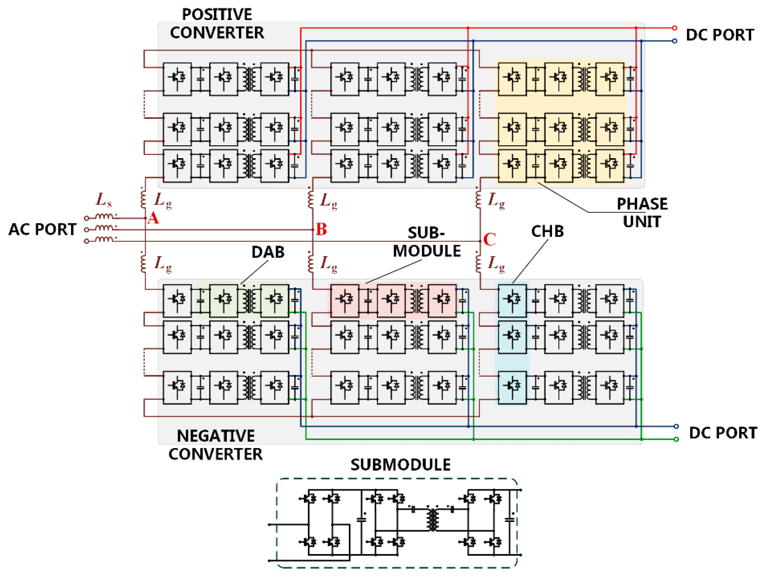
2. The Full-Order Small-Signal Model of MP-PET

Figure 1 shows the topology structure of cascaded H-bridge MP-PET, which consists of three parts: input stage, isolation stage, and output stage. The input stage adopts the cascade structure of power submodules, which can reduce the voltage tolerance level of switching devices in each power submodule. Meanwhile, the voltage and current on the input side can be operated with the same phase through effective control. The isolation stage adopts resonant dual-active-bridge (DAB) topology to provide an interface for dc load and the energy can bidirectionally flow through power control. When the DAB operates in open-loop resonant mode, its internal switching devices can realize the zero-current-switching (ZCS) so as to reduce power loss and improve system efficiency. The output stage connects each independent bidirectional dc-dc converter directly in parallel with the dc bus to the load side. To sum up, a three-port circuit is provided in this paper that can connect to different types of power, energy storage, and load equipment. Furthermore, it is worth mentioning that this topology is designed for practical engineering and has already been put into operation.

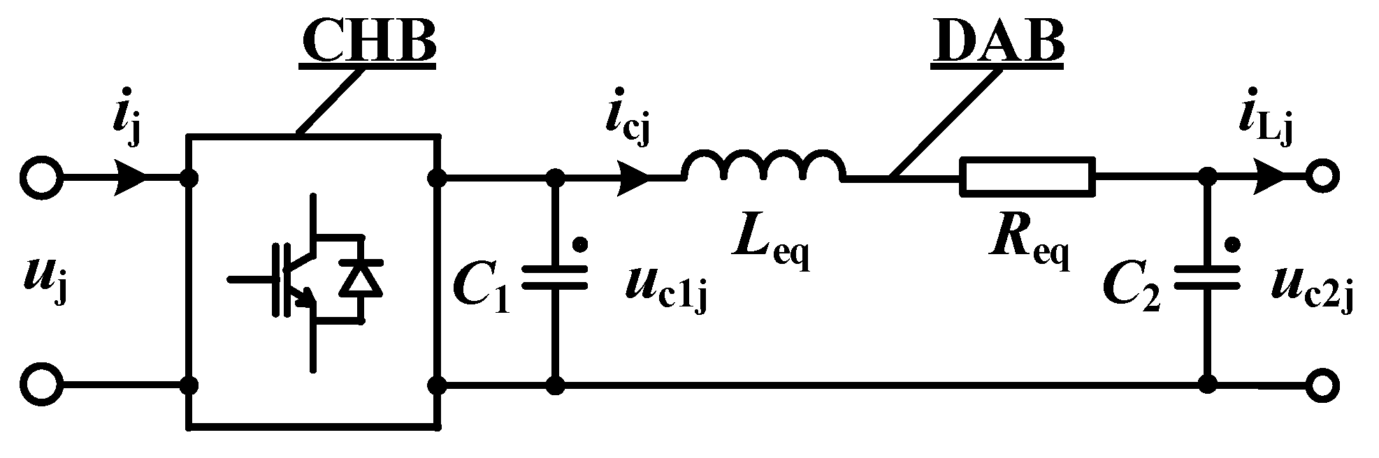
2.1. PET Small Signal Modeling Analysis

The resonant DAB high-frequency link in Figure 1 can be equivalent to a first-order RL circuit [19] by means of the current average method as shown in Figure 2, where R_eq = π²R_loss/8, L_eq = π²L_res/4. R_loss shows the leakage resistance of the DAB and L_res represents the resonant inductor of DAB.

As shown in Figure 1 and Figure 2, L_s, R_s represents the grid side inductor and resistor, respectively. C_eq indicates the equivalent capacitor from the converter side to the ground and L_g, R_g represents the bridge arm inductor and resistor. The DAB is modeled by an inductance L_eq, a resistance R_eq and capacitor C₁, C₂, which indicates the primary and secondary capacitance values of the transformer. In this paper, the PET single-phase circuit is taken as an example for modeling and analysis. Based on the KVL and KCL circuit laws, the stage equations can be listed as (where j represents phase a, b, c)

$$u_{\mathrm{j}}-L_{\mathrm{s}}\frac{\mathrm{d}\left(i_{\mathrm{j}\_\mathrm{up}}+i_{\mathrm{j}\_\mathrm{low}}\right)}{\mathrm{d}t}-R_{\mathrm{s}}\left(i_{\mathrm{j}\_\mathrm{up}}+i_{\mathrm{j}\_\mathrm{low}}\right)-L_{\mathrm{g}}\frac{\mathrm{d}{i}_{\mathrm{j}\_\mathrm{up}}}{\mathrm{d}t}-R_{\mathrm{g}}{i}_{\mathrm{j}\_\mathrm{up}}=S_{\mathrm{j}\_\mathrm{up}}{u}_{\mathrm{c}1\mathrm{j}\_\mathrm{up}}N$$

(1)

$$i_{\mathrm{j}\_\mathrm{up}}{S}_{\mathrm{j}\_\mathrm{up}}-C_1\frac{\mathrm{d}{u}_{\mathrm{c}1\mathrm{j}\_\mathrm{up}}}{\mathrm{d}t}=i_{\mathrm{cj}\_\mathrm{up}}$$

(2)

$$i_{\mathrm{cj}\_\mathrm{up}}-i_{\mathrm{Lj}\_\mathrm{up}}=C_2\frac{\mathrm{d}{u}_{\mathrm{c}2\mathrm{j}\_\mathrm{up}}}{\mathrm{d}t}$$

(3)

$$u_{\mathrm{c}1\mathrm{j}\_\mathrm{up}}-u_{\mathrm{c}2\mathrm{j}\_\mathrm{up}}=L_{\mathrm{eq}}\frac{\mathrm{d}{i}_{\mathrm{cj}\_\mathrm{up}}}{\mathrm{d}t}+R_{\mathrm{eq}}{i}_{\mathrm{cj}\_\mathrm{up}}$$

(4)

$$u_{\mathrm{j}}-L_{\mathrm{s}}\frac{\mathrm{d}{i}_{\mathrm{j}\_\mathrm{sum}}}{\mathrm{d}t}-R_{\mathrm{s}}{i}_{\mathrm{j}\_\mathrm{sum}}=v_{\mathrm{j}}$$

(5)

$$i_{\mathrm{j}\_\mathrm{sum}}=i_{\mathrm{j}\_\mathrm{up}}+i_{\mathrm{j}\_\mathrm{low}}+C_{\mathrm{eq}}\frac{\mathrm{d}{v}_{\mathrm{j}}}{\mathrm{d}t}$$

(6)

where the subscript “up” and “low” represent the positive and negative converter, respectively. The subscript “sum” represents a common coupling side of the two converters. Furthermore, u_j, i_j stands for the grid side voltage and current, respectively and v_j shows the ac voltage of the converter. In the DAB, i_cj indicates the equivalent dc current of the DAB and u_c1, u_c2 represents the capacitor voltage of the input and output stage. In addition, N shows the number of bridge arm submodules. S shows a modulation reference wave. ω represents the grid angular frequency and i_Lj means the load current.

The d—q axis transformer for the above equations and small signal linear analysis, which is equivalent to the above variables as $x=X+\tilde{x}$, are performed. X indicates the steady state component and $\tilde{x}$ represents the small disturbance component. The system state equations can be obtained as:

$$\frac{3}{2}\left(I_{\mathrm{d}\_\mathrm{up}}{\tilde{S}}_{\mathrm{d}\_\mathrm{up}}+m_{\mathrm{d}\_\mathrm{up}}{\tilde{i}}_{\mathrm{d}\_\mathrm{up}}+I_{\mathrm{q}\_\mathrm{up}}{\tilde{S}}_{\mathrm{q}\_\mathrm{up}}+m_{\mathrm{q}\_\mathrm{up}}{\tilde{i}}_{\mathrm{q}\_\mathrm{up}}\right)-3C_1\frac{\mathrm{d}{\tilde{u}}_{\mathrm{c}1\_\mathrm{up}}}{\mathrm{d}t}=3{\tilde{i}}_{\mathrm{c}\_\mathrm{up}}$$

(7)

$$3{\tilde{i}}_{\mathrm{c}\_\mathrm{up}}-3{\tilde{i}}_{\mathrm{L}\_\mathrm{up}}=3C_2\frac{\mathrm{d}{\tilde{u}}_{\mathrm{c}2\_\mathrm{up}}}{\mathrm{d}t}$$

(8)

$$3{\tilde{u}}_{\mathrm{c}1\_\mathrm{up}}-3{\tilde{u}}_{\mathrm{c}2\_\mathrm{up}}=L_{\mathrm{eq}}\frac{3\mathrm{d}{\tilde{i}}_{\mathrm{c}\_\mathrm{up}}}{\mathrm{d}t}+R_{\mathrm{eq}}3{\tilde{i}}_{\mathrm{c}\_\mathrm{up}}$$

(9)

$$\{\begin{array}{c}{\tilde{v}}_{\mathrm{d}}-L_{\mathrm{g}}\frac{\mathrm{d}{\tilde{i}}_{\mathrm{d}\_\mathrm{up}}}{\mathrm{d}t}+L_{\mathrm{g}}\omega {\tilde{i}}_{\mathrm{q}\_\mathrm{up}}-R_{\mathrm{g}}{\tilde{i}}_{\mathrm{d}\_\mathrm{up}}=N\left[{\tilde{u}}_{\mathrm{ref}\_\mathrm{d}\_\mathrm{up}}+{\tilde{u}}_{\mathrm{c}1\_\mathrm{up}}{m}_{\mathrm{d}\_\mathrm{up}}\right]\\ {\tilde{v}}_{\mathrm{q}}-L_{\mathrm{g}}\frac{\mathrm{d}{\tilde{i}}_{\mathrm{q}\_\mathrm{up}}}{\mathrm{d}t}-L_{\mathrm{g}}\omega {\tilde{i}}_{\mathrm{d}\_\mathrm{up}}-R_{\mathrm{g}}{\tilde{i}}_{\mathrm{q}\_\mathrm{up}}=N\left[{\tilde{u}}_{\mathrm{ref}\_\mathrm{q}\_\mathrm{up}}+{\tilde{u}}_{\mathrm{c}1\_\mathrm{up}}{m}_{\mathrm{q}\_\mathrm{up}}\right]\end{array}$$

(10)

$$\{\begin{array}{c}{\tilde{u}}_{\mathrm{d}}-L_{\mathrm{s}}\frac{\mathrm{d}{\tilde{i}}_{\mathrm{d}\_\mathrm{sum}}}{\mathrm{d}t}+L_{\mathrm{s}}\omega {\tilde{i}}_{\mathrm{q}\_\mathrm{sum}}-R_{\mathrm{s}}{\tilde{i}}_{\mathrm{d}\_\mathrm{sum}}={\tilde{v}}_{\mathrm{d}}\\ {\tilde{u}}_{\mathrm{q}}-L_{\mathrm{s}}\frac{\mathrm{d}{\tilde{i}}_{\mathrm{q}\_\mathrm{sum}}}{\mathrm{d}t}-L_{\mathrm{s}}\omega {\tilde{i}}_{\mathrm{d}\_\mathrm{sum}}-R_{\mathrm{s}}{\tilde{i}}_{\mathrm{q}\_\mathrm{sum}}={\tilde{v}}_{\mathrm{q}}\end{array}$$

(11)

$$\{\begin{array}{c}{\tilde{i}}_{\mathrm{d}\_\mathrm{sum}}={\tilde{i}}_{\mathrm{d}\_\mathrm{up}}+{\tilde{i}}_{\mathrm{d}\_\mathrm{low}}+C_{\mathrm{eq}}\frac{\mathrm{d}{\tilde{v}}_{\mathrm{d}}}{\mathrm{d}t}-C_{\mathrm{eq}}\omega {\tilde{v}}_{\mathrm{q}}\\ {\tilde{i}}_{\mathrm{q}\_\mathrm{sum}}={\tilde{i}}_{\mathrm{q}\_\mathrm{up}}+{\tilde{i}}_{\mathrm{q}\_\mathrm{low}}+C_{\mathrm{eq}}\frac{\mathrm{d}{\tilde{v}}_{\mathrm{q}}}{\mathrm{d}t}-C_{\mathrm{eq}}\omega {\tilde{v}}_{\mathrm{d}}\end{array}$$

(12)

where:

$$\{\begin{array}{c}{m}_{\mathrm{d}\_\mathrm{up}}=\frac{U_{\mathrm{d}}+\omega L_{\mathrm{s}}\left(I_{\mathrm{q}\_\mathrm{up}}+I_{\mathrm{q}\_\mathrm{low}}\right)-R_{\mathrm{s}}\left(I_{\mathrm{d}\_\mathrm{up}}+I_{\mathrm{d}\_\mathrm{low}}\right)}{N{U}_{\mathrm{dc}1}}+\frac{\omega L_{\mathrm{g}}{I}_{\mathrm{q}\_\mathrm{up}}-R_{\mathrm{g}}{I}_{\mathrm{d}\_\mathrm{up}}}{N{U}_{\mathrm{dc}1}}\\ m_{\mathrm{q}\_\mathrm{up}}=\frac{U_{\mathrm{q}}-\omega L_{\mathrm{s}}\left(I_{\mathrm{d}\_\mathrm{up}}+I_{\mathrm{d}\_\mathrm{low}}\right)-R_{\mathrm{s}}\left(I_{\mathrm{q}\_\mathrm{up}}+I_{\mathrm{q}\_\mathrm{low}}\right)}{N{U}_{\mathrm{dc}1}}-\frac{\omega L_{\mathrm{g}}{I}_{\mathrm{d}\_\mathrm{up}}+R_{\mathrm{g}}{I}_{\mathrm{q}\_\mathrm{up}}}{N{U}_{\mathrm{dc}1}}\end{array}$$

By converting Equations (7)–(12) into matrix form, the PET modeling can be written as follows:

$$\frac{\mathrm{d}\tilde{x}}{\mathrm{d}t}=A\tilde{x}+B\tilde{u}$$

(13)

where:

$$\tilde{x}=\left[\begin{array}{ccccccc}{\tilde{i}}_{\mathrm{c}\_\mathrm{up}}& {\tilde{i}}_{\mathrm{d}\_\mathrm{up}}& {\tilde{i}}_{\mathrm{q}\_\mathrm{up}}& {\tilde{u}}_{\mathrm{c}1\_\mathrm{up}}& {\tilde{u}}_{\mathrm{c}2\_\mathrm{up}}& {\tilde{i}}_{\mathrm{c}\_\mathrm{low}}& {\tilde{i}}_{\mathrm{d}\_\mathrm{low}}\\ {\tilde{i}}_{\mathrm{q}\_\mathrm{low}}& {\tilde{u}}_{\mathrm{c}1\_\mathrm{low}}& {\tilde{u}}_{\mathrm{c}2\_\mathrm{low}}& {\tilde{i}}_{\mathrm{d}\_\mathrm{sum}}& {\tilde{i}}_{\mathrm{q}\_\mathrm{sum}}& {\tilde{v}}_{\mathrm{d}}& {\tilde{v}}_{\mathrm{q}}\end{array}\right]$$

$$\tilde{u}=\left[\begin{array}{cccc}{\tilde{i}}_{\mathrm{L}\_\mathrm{up}}& {\tilde{u}}_{\mathrm{ref}\_\mathrm{d}\_\mathrm{up}}& {\tilde{u}}_{\mathrm{ref}\_\mathrm{q}\_\mathrm{up}}& {\tilde{i}}_{\mathrm{L}\_\mathrm{low}}\\ {\tilde{u}}_{\mathrm{ref}\_\mathrm{d}\_\mathrm{low}}& {\tilde{u}}_{\mathrm{ref}\_\mathrm{q}\_\mathrm{low}}& {\tilde{u}}_{\mathrm{d}}& {\tilde{u}}_{\mathrm{q}}\end{array}\right]$$

where $\tilde{x}$ represents state variables and $\tilde{u}$ indicates input variables, which provide a controller interface. The expression of A and B are shown as following where the matrix coefficients can be found in the Appendix A:

$$A=\left[\begin{array}{ccc}{A}_{11}& 0& A_{13}\\ 0& A_{22}& A_{23}\\ A_{31}& A_{32}& A_{33}\end{array}\right]B=\left[\begin{array}{ccc}{B}_{11}& 0& 0\\ 0& B_{22}& 0\\ 0& 0& B_{33}\end{array}\right]$$

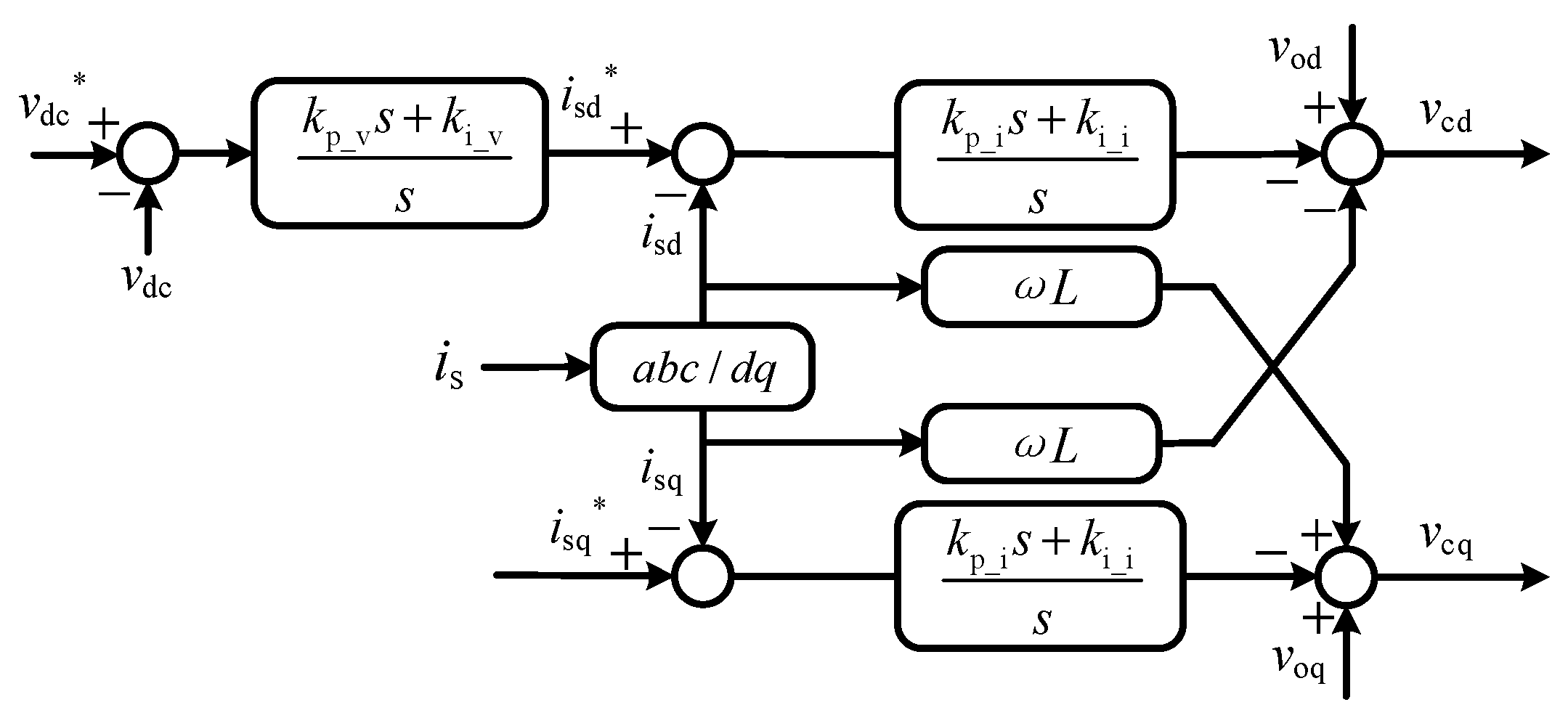
2.2. Control system Small Signal Modeling Analysis

As shown in Figure 3, this paper adopts the d-q decoupling double closed-loop control strategy. The output loop is a dc bus voltage feedback loop and the inner loop is a grid current feedback loop. Therefore, the PET control system has six PI controllers, which means having six state variables (each converter has three). Among them, the voltage loop has one state and the current loop has two.

Where the small signal equation of state can be listed as:

$$\frac{\mathrm{d}{\tilde{x}}_1}{\mathrm{d}t}=-{\tilde{u}}_{\mathrm{dc}}{K}_{\mathrm{i}\_\mathrm{v}}$$

(14)

$$\frac{\mathrm{d}{\tilde{x}}_2}{\mathrm{d}t}=\left({\tilde{x}}_1-K_{\mathrm{p}\_\mathrm{v}}{\tilde{u}}_{\mathrm{dc}}-{\tilde{i}}_{\mathrm{d}}\right)K_{\mathrm{i}\_\mathrm{i}}$$

(15)

$$\frac{\mathrm{d}{\tilde{x}}_3}{\mathrm{d}t}=-{\tilde{i}}_{\mathrm{q}}{K}_{\mathrm{i}\_\mathrm{i}}$$

(16)

$${\tilde{u}}_{\mathrm{ref}\_\mathrm{d}}=\frac{{\tilde{v}}_{\mathrm{d}}-{\tilde{x}}_2-\left({\tilde{x}}_1-K_{\mathrm{p}\_\mathrm{v}}{\tilde{u}}_{\mathrm{dc}}-{\tilde{i}}_{\mathrm{d}}\right)K_{\mathrm{p}\_\mathrm{i}}+{\tilde{i}}_{\mathrm{q}}\omega L}{N}$$

(17)

$${\tilde{u}}_{\mathrm{ref}\_\mathrm{q}}=\frac{{\tilde{v}}_{\mathrm{q}}-{\tilde{x}}_3+{\tilde{i}}_{\mathrm{q}}{K}_{\mathrm{p}\_\mathrm{i}}-{\tilde{i}}_{\mathrm{d}}\omega L}{N}$$

(18)

where K_{p_v}, K_{i_v}, K_{p_i}, K_{i_i} represent the controller coefficient of PET.

The state space equation of the controller system can be converted by Equations (14)–(18) into the following form:

$$\{\begin{array}{c}\frac{\mathrm{d}{\tilde{x}}_{\mathrm{c}}}{\mathrm{d}t}=A_{\mathrm{c}}{\tilde{x}}_{\mathrm{c}}+B_{\mathrm{c}}{\tilde{u}}_{\mathrm{c}}\\ {\tilde{y}}_{\mathrm{c}}=C_{\mathrm{c}}{\tilde{x}}_{\mathrm{c}}+D_{\mathrm{c}}{\tilde{u}}_{\mathrm{c}}\end{array}$$

(19)

where:

$${\tilde{x}}_{\mathrm{c}}=\left[\begin{array}{cccccc}{\tilde{x}}_1& {\tilde{x}}_2& {\tilde{x}}_3& {\tilde{x}}_1\prime & {\tilde{x}}_2\prime & {\tilde{x}}_3\prime \end{array}\right]$$

$${\tilde{u}}_{\mathrm{c}}=\left[\begin{array}{cccccccc}{\tilde{i}}_{\mathrm{d}\_\mathrm{up}}& {\tilde{i}}_{\mathrm{q}\_\mathrm{up}}& {\tilde{u}}_{\mathrm{dc}\_\mathrm{up}}& {\tilde{i}}_{\mathrm{d}\_\mathrm{low}}& {\tilde{i}}_{\mathrm{q}\_\mathrm{low}}& {\tilde{u}}_{\mathrm{dc}\_\mathrm{low}}& {\tilde{v}}_{\mathrm{d}}& {\tilde{v}}_{\mathrm{q}}\end{array}\right]$$

$${\tilde{y}}_{\mathrm{c}}=\left[\begin{array}{cccc}{\tilde{u}}_{\mathrm{ref}\_\mathrm{d}\_\mathrm{up}}& {\tilde{u}}_{\mathrm{ref}\_\mathrm{q}\_\mathrm{up}}& {\tilde{u}}_{\mathrm{ref}\_\mathrm{d}\_\mathrm{low}}& {\tilde{u}}_{\mathrm{ref}\_\mathrm{q}\_\mathrm{low}}\end{array}\right]$$

where ${\tilde{x}}_{\mathrm{c}}$ represents state variables of the control system. ${\tilde{u}}_{\mathrm{c}}$, ${\tilde{y}}_{\mathrm{c}}$ indicates input and output variables of the control system. The expression of A_c, B_c, C_c, D_c can be found in the Appendix A.

The state space equation for the whole system can be obtained by combing Equations (13) and (19), which is expressed as follows:

$$\left[\begin{array}{c}\frac{\mathrm{d}\tilde{x}}{\mathrm{d}t}\\ \frac{\mathrm{d}{\tilde{x}}_{\mathrm{c}}}{\mathrm{d}t}\end{array}\right]=\left[\begin{array}{cc}A& 0\\ 0& A_{\mathrm{c}}\end{array}\right]\left[\begin{array}{c}\tilde{x}\\ {\tilde{x}}_{\mathrm{c}}\end{array}\right]+\left[\begin{array}{ccc}{B}_1& B_2& 0\\ 0& 0& B_{\mathrm{c}}\end{array}\right]\left[\begin{array}{c}{\tilde{u}}_1\\ {\tilde{u}}_2\\ {\tilde{u}}_{\mathrm{c}}\end{array}\right]$$

(20)

where B₁ contains the 2,3,5,6 column vectors of B and B₂ contains the 1,4,7,8 column vectors of B, where both are 14 × 4 matrices. ${\tilde{u}}_1$ contains the 2,3,5,6 variables of $\tilde{u}$ and ${\tilde{u}}_2$ contains the 1,4,7,8 variables of $\tilde{u}$, where both are 14 × 1 matrices.

By introducing a matrix E, the equation can be described as:

$$\{\begin{array}{c}{\tilde{u}}_1={\tilde{y}}_{\mathrm{c}}=C_{\mathrm{c}}{\tilde{x}}_{\mathrm{c}}+D_{\mathrm{c}}{\tilde{u}}_{\mathrm{c}}\\ {\tilde{u}}_{\mathrm{c}}=E\tilde{x}\end{array}$$

(21)

Then, putting Equation (21) into Equation (20), we get the final state equation.

$$\left[\begin{array}{c}\frac{\mathrm{d}\tilde{x}}{\mathrm{d}t}\\ \frac{\mathrm{d}{\tilde{x}}_{\mathrm{c}}}{\mathrm{d}t}\end{array}\right]=\left[\begin{array}{cc}A+B_1{D}_{\mathrm{c}}E& B_1{C}_{\mathrm{c}}\\ B_{\mathrm{c}}E& A_{\mathrm{c}}\end{array}\right]\left[\begin{array}{c}\tilde{x}\\ {\tilde{x}}_{\mathrm{c}}\end{array}\right]+\left[\begin{array}{c}{B}_2\\ 0\end{array}\right]{\tilde{u}}_2$$

(22)

where:

$${\tilde{u}}_2=\left[\begin{array}{cccc}{\tilde{i}}_{\mathrm{L}\_\mathrm{up}}& {\tilde{i}}_{\mathrm{L}\_\mathrm{low}}& {\tilde{u}}_{\mathrm{d}}& {\tilde{u}}_{\mathrm{q}}\end{array}\right]$$

All of the matrix coefficients can be found in the Appendix A.

3. The Reduced-Order Small-Signal Model of MP-PET

In order to quickly and effectively analyze the dynamic response on system dc bus voltage, this paper uses the participation factor analysis method to establish a reduced-order small signal model based on the full-order mathematical model, which is derived from Section 2. It makes the order reduce from 20 to 10 (50%). Hence, the simplified model could not only precisely describe the dynamic behavior of the dc bus voltage but also greatly reduce the computational complexity of the system model. Furthermore, it should be specially explained that the small signal simplified model obtained by the traditional method [18] is based on the steady-state power balance relationship of the converter, which cannot accurately reflect its dynamic performance. In this paper, a new simplified small signal model is constructed by using instantaneous variable theory. The model has the same order as the traditional reduced-order model, but the description of the dc voltage motion modes is more accurate.

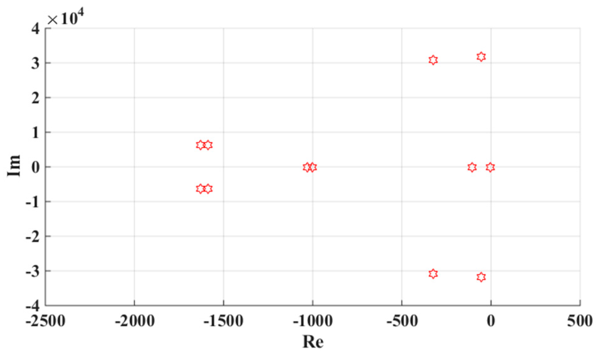
3.1. PET Small Signal Model Eigenvalue Analysis

Modal analysis based on the system linearization model is a very effective method for small signal stability analysis of a power system [20]. It could offer much important information, such as participation factors that provide the research foundation for a model reduction. As participation factor is an important parameter that could measure the influence of each state variable on the eigenvalue and reflect the relative participation of each state variable to the motion mode described by a certain eigenvalue, it is necessary to extract the eigenvalue that has a dominant influence on the dc bus voltage by parameter factor analysis, and select the state variables that have a strong correlation to the above eigenvalues. In summary, the reduced-order model of PET contains all state information related to the dominant mode of the dc bus voltage that serves as the reference for model simplification.

$$p_{\mathrm{ki}}=\frac{\partial {\lambda }_{\mathrm{i}}}{\partial a_{\mathrm{kk}}}={\psi }_{\mathrm{ik}}{\varphi }_{\mathrm{ik}}$$

(23)

where p_ki represents participation factors, λ_i shows the eigenvalue root, a_kk indicates diagonal elements of the state matrix, ψ_ik, and φ_ik represent the left and right normalized eigenvector elements, respectively. Considering the normalization of eigenvectors, the sum of participation factors associated with any motion mode or state variable is equal to 1. Thus, with increasingly higher participation factors, the degree of participation is higher.

As shown in

Table 1. The eigenvalues of MP-PET

Characteristic Root	Value
λ1, λ2	−53.32 ± 31738.43i
λ3, λ4	−322.49 ± 30873.29i
λ5	−45609.81 + 0i
λ6	−46450.81 + 0i
λ7, λ8	−1628.59 ± 6403.34i
λ9, λ10	−1587.14 ± 6303.85i
λ11	−1028.17 + 0i
λ12	−1001.67 + 0i
λ13	−107.92 + 0i
λ14	−107.89 + 0i
λ15	−50008 + 0i
λ16	−50008 + 0i
λ17	−2 + 0i
λ18	−2 + 0i
λ19	−1.99 + 0i
λ20	−1.99 + 0i

, substituting parameters from

Table 2. Main circuit parameters of MP-PET.

MP-PET Configuration	Value
Rated apparent power [MVA]	3
dc voltage [V]	1900
The line to line voltage of grid (RMS) [kV]	10
Number of submodules per arm	5
Number of redundant submodules per arm	1
Grid side inductance [mH]	1
Arm inductance [mH]	10
CHB capacitance [mF]	1
DAB capacitance [mF]	1
Resonant inductance [μH]	20
Resonant capacitance [μF]	50
Resonant frequency [kHz]	5
CHB switching frequency [Hz]	800
Transformer ratio	1:1

into Equation (23), the eigenvalues and the participation factors of PET have been calculated. Besides, Figure 4 presents the distributed situation of the eigenvalues which shows that the PET eigenvalues can be classified into eight groups.

According to the participation factors listed in

Table A1. Participation factor value of MP-PET.

	λ1	λ2	λ3	λ4	λ5	λ6	λ7	λ8	λ9	λ10	λ11	λ12	λ13	λ14	λ15	λ16	λ17	λ18	λ19	λ20
ic_up	0.0000	0.0000	0.0003	0.0003	0.0005	0.0004	0.2587	0.2587	0.2580	0.2580	0.0172	0.0159	0.0000	0.0000	0.0000	0.0000	0.0000	0.0000	0.0000	0.0000
id_up	0.0009	0.0009	0.0061	0.0061	0.5543	0.5394	0.0121	0.0121	0.0107	0.0107	0.0191	0.0183	0.0002	0.0002	0.0000	0.0000	0.0000	0.0000	0.0000	0.0000
iq_up	0.0000	0.0000	0.0000	0.0000	0.0000	0.0000	0.0000	0.0000	0.0000	0.0000	0.0000	0.0000	0.0000	0.0000	1.0376	0.0376	0.0000	0.0000	0.0000	0.0000
uc1_up	0.0017	0.0017	0.0118	0.0118	0.0516	0.0399	0.1629	0.1629	0.1487	0.1487	0.2910	0.2837	0.0303	0.0302	0.0000	0.0000	0.0000	0.0000	0.0000	0.0000
uc2_up	0.0000	0.0000	0.0000	0.0000	0.0000	0.0000	0.1172	0.1172	0.1207	0.1207	0.3211	0.3131	0.0310	0.0309	0.0000	0.0000	0.0000	0.0000	0.0000	0.0000
ic_low	0.0000	0.0000	0.0003	0.0003	0.0005	0.0004	0.2587	0.2587	0.2580	0.2580	0.0172	0.0159	0.0000	0.0000	0.0000	0.0000	0.0000	0.0000	0.0000	0.0000
id_low	0.0009	0.0009	0.0061	0.0061	0.5543	0.5394	0.0121	0.0121	0.0107	0.0107	0.0191	0.0183	0.0002	0.0002	0.0000	0.0000	0.0000	0.0000	0.0000	0.0000
iq_low	0.0000	0.0000	0.0000	0.0000	0.0000	0.0000	0.0000	0.0000	0.0000	0.0000	0.0000	0.0000	0.0000	0.0000	0.0376	1.0376	0.0000	0.0000	0.0000	0.0000
uc1_low	0.0017	0.0017	0.0118	0.0118	0.0516	0.0399	0.1629	0.1629	0.1487	0.1487	0.2910	0.2837	0.0303	0.0302	0.0000	0.0000	0.0000	0.0000	0.0000	0.0000
uc2_low	0.0000	0.0000	0.0000	0.0000	0.0000	0.0000	0.1172	0.1172	0.1207	0.1207	0.3211	0.3131	0.0310	0.0309	0.0000	0.0000	0.0000	0.0000	0.0000	0.0000
id_sum	0.0729	0.0729	0.4744	0.4744	0.0061	0.0000	0.0179	0.0179	0.0000	0.0000	0.0267	0.0000	0.0000	0.0003	0.0000	0.0000	0.0000	0.0000	0.0000	0.0000
iq_sum	0.4491	0.4491	0.0692	0.0692	0.0000	0.0000	0.0000	0.0000	0.0000	0.0000	0.0000	0.0000	0.0000	0.0000	0.0000	0.0000	0.0000	0.0000	0.0000	0.0000
vd	0.0701	0.0701	0.4555	0.4555	0.0128	0.0000	0.0008	0.0008	0.0000	0.0000	0.0000	0.0000	0.0000	0.0000	0.0000	0.0000	0.0000	0.0000	0.0000	0.0000
vq	0.4491	0.4491	0.0692	0.0692	0.0000	0.0000	0.0000	0.0000	0.0000	0.0000	0.0000	0.0000	0.0000	0.0000	0.0000	0.0000	0.0000	0.0000	0.0000	0.0000
x1	0.0000	0.0000	0.0000	0.0000	0.0001	0.0001	0.0009	0.0009	0.0008	0.0008	0.0624	0.0627	0.5613	0.5610	0.0000	0.0000	0.0002	0.0002	0.0000	0.0000
x2	0.0000	0.0000	0.0000	0.0000	0.0000	0.0000	0.0000	0.0000	0.0000	0.0000	0.0000	0.0000	0.0002	0.0002	0.0000	0.0000	0.5002	0.5002	0.0000	0.0000
x3	0.0000	0.0000	0.0000	0.0000	0.0000	0.0000	0.0000	0.0000	0.0000	0.0000	0.0000	0.0000	0.0000	0.0000	0.0000	0.0000	0.0000	0.0000	1.1691	0.1690
x1′	0.0000	0.0000	0.0000	0.0000	0.0001	0.0001	0.0009	0.0009	0.0008	0.0008	0.0624	0.0627	0.5613	0.5610	0.0000	0.0000	0.0002	0.0002	0.0000	0.0000
x2′	0.0000	0.0000	0.0000	0.0000	0.0000	0.0000	0.0000	0.0000	0.0000	0.0000	0.0000	0.0000	0.0000	0.0000	0.0000	0.0000	0.5002	0.5002	0.0001	0.0001
x3′	0.0000	0.0000	0.0000	0.0000	0.0000	0.0000	0.0000	0.0000	0.0000	0.0000	0.0000	0.0000	0.0000	0.0000	0.0000	0.0000	0.0000	0.0000	0.1690	1.1690

, it can be known that the first group of characteristic roots λ₁, λ₂ mainly affect the q-axis current and q-axis voltage state variables at the grid side. The second group of characteristic roots λ₃, λ₄ influence the d-axis current and voltage state variables at the grid side. The third group of characteristic roots λ₅, λ₆ have a strong correlation with the d-axis current of the bridge arm and the dc bus voltage state variables from the DAB primary side. Meanwhile, the fourth group of characteristic roots λ₇, λ₈, λ₉, λ₁₀ mainly affect the equivalent dc current of the resonant circuit and the state variables of dc bus voltage from the primary and secondary side. The fifth group of characteristic roots λ₁₁, λ₁₂, λ₁₃, λ₁₄ mainly influence the internal state variables of the dc voltage control loop and state variables of dc bus voltage. The sixth group of characteristic roots λ₁₅, λ₁₆ are highly relevant to the q-axis current state variables of the bridge arm. Furthermore, the seventh group characteristic roots λ₁₇, λ₁₈ mainly affect the internal state variables of the d-axis current control loop. The eighth group characteristic roots λ₁₉, λ₂₀ mainly influence the internal state variables of the q-axis current control loop. In conclusion, the characteristic roots that have a strong correlation with the dc bus voltage are λ₅, λ₆, λ₇, λ₈, λ₉, λ₁₀, λ₁₁, λ₁₂, λ₁₃, λ₁₄. Thus, when the reduced-order model contains ten motion modes corresponding to the above ten characteristic roots, it can accurately reflect the dynamic voltage response of the dc bus of PET under external perturbation.

In addition, according to Table A1, the system state variables i_{d_up} and i_{d_low} have a strong correlation with the characteristic roots λ₅, λ₆. The state variables i_{c_up} and i_{c_low} are connected with the characteristic roots λ₇, λ₈, λ₉, λ₁₀. The state variables x₁ and x_1′ have an influence on the characteristic roots λ₁₁, λ₁₂, λ₁₃, λ₁₄. Hence, in order to maintain the precision of the reduced-order model, it is necessary to retain the above six state variables and ignore the remaining variables to ensure that the reduced-order model of MP-PET contains the relevant state information related to the solution of the dominant characteristic roots λ₅~λ₁₄.

3.2. PET Small Signal Model Simplification

According to the analysis in the previous section, the state variables that have a low correlation with dc bus voltage should be excluded. Thus, the capacitance–voltage and current state variables from the grid side are ignored, which means the LCL filter branch is simplified to a pure inductance structure. Furthermore, the reduced-order model should also ignore all the state variables associated with the q-axis and the inner loop of the controller system. To sum up, the small signal model can be simplified as follows:

$${\tilde{u}}_{\mathrm{d}}-\left(L_{\mathrm{g}}+L_{\mathrm{s}}\right)\frac{\mathrm{d}{\tilde{i}}_{\mathrm{d}\_\mathrm{up}}}{\mathrm{d}t}-\left(R_{\mathrm{g}}+R_{\mathrm{s}}\right){\tilde{i}}_{\mathrm{d}\_\mathrm{up}}=N\left[{\tilde{u}}_{\mathrm{ref}\_\mathrm{d}\_\mathrm{up}}+{\tilde{u}}_{\mathrm{c}1\_\mathrm{up}}{m}_{\mathrm{d}\_\mathrm{up}}\right]$$

(24)

$$\frac{3}{2}\left(I_{\mathrm{d}\_\mathrm{up}}{\tilde{S}}_{\mathrm{d}\_\mathrm{up}}+m_{\mathrm{d}\_\mathrm{up}}{\tilde{i}}_{\mathrm{d}\_\mathrm{up}}\right)-3C_1\frac{\mathrm{d}{\tilde{u}}_{\mathrm{c}1\_\mathrm{up}}}{\mathrm{d}t}=3{\tilde{i}}_{\mathrm{c}\_\mathrm{up}}$$

(25)

$$3{\tilde{i}}_{\mathrm{c}\_\mathrm{up}}-3{\tilde{i}}_{\mathrm{L}\_\mathrm{up}}=3C_2\frac{\mathrm{d}{\tilde{u}}_{\mathrm{c}2\_\mathrm{up}}}{\mathrm{d}t}$$

(26)

$$3{\tilde{u}}_{\mathrm{c}1\_\mathrm{up}}-3{\tilde{u}}_{\mathrm{c}2\_\mathrm{up}}=L_{\mathrm{eq}}\frac{3\mathrm{d}{\tilde{i}}_{\mathrm{c}\_\mathrm{up}}}{\mathrm{d}t}+R_{\mathrm{eq}}3{\tilde{i}}_{\mathrm{c}\_\mathrm{up}}$$

(27)

$$\frac{\mathrm{d}{\tilde{x}}_1}{\mathrm{d}t}=-{\tilde{u}}_{\mathrm{dc}}{K}_{\mathrm{i}\_\mathrm{v}}$$

(28)

$${\tilde{u}}_{\mathrm{ref}\_\mathrm{d}}=\frac{{\tilde{u}}_{\mathrm{d}}-\left({\tilde{x}}_1-K_{\mathrm{p}\_\mathrm{v}}{\tilde{u}}_{\mathrm{dc}}-{\tilde{i}}_{\mathrm{d}}\right)K_{\mathrm{p}\_\mathrm{i}}}{N}$$

(29)

where:

$$m_{\mathrm{d}\_\mathrm{up}}=\frac{U_{\mathrm{d}}-R_{\mathrm{s}}\left(I_{\mathrm{d}\_\mathrm{up}}+I_{\mathrm{d}\_\mathrm{low}}\right)-R_{\mathrm{g}}{I}_{\mathrm{d}\_\mathrm{up}}}{N{U}_{\mathrm{dc}1}}$$

By converting Equations (24)–(27) into a matrix.

$$\frac{\mathrm{d}\tilde{x}}{\mathrm{d}t}=A_{\mathrm{s}}\tilde{x}+B_{\mathrm{s}}\tilde{u}$$

(30)

The state variables and input variables, respectively, are shown as follows:

$$\tilde{x}=\left[\begin{array}{cccc}{\tilde{i}}_{\mathrm{c}\_\mathrm{up}}& {\tilde{i}}_{\mathrm{d}\_\mathrm{up}}& {\tilde{u}}_{\mathrm{c}1\_\mathrm{up}}& {\tilde{u}}_{\mathrm{c}2\_\mathrm{up}}\\ {\tilde{i}}_{\mathrm{c}\_\mathrm{low}}& {\tilde{i}}_{\mathrm{d}\_\mathrm{low}}& {\tilde{u}}_{\mathrm{c}1\_\mathrm{low}}& {\tilde{u}}_{\mathrm{c}2\_\mathrm{low}}\end{array}\right]$$

$$\tilde{u}=\left[\begin{array}{cccc}{\tilde{i}}_{\mathrm{L}\_\mathrm{up}}& {\tilde{u}}_{\mathrm{ref}\_\mathrm{d}\_\mathrm{up}}& {\tilde{i}}_{\mathrm{L}\_\mathrm{low}}& {\tilde{u}}_{\mathrm{ref}\_\mathrm{d}\_\mathrm{low}}\end{array}\right]$$

The expression of the matrix coefficients from A_s and B_s can be found in the Appendix A:

$$A_{\mathrm{s}}=\left[\begin{array}{cc}{A}_{\mathrm{s}11}& 0\\ 0& A_{\mathrm{s}22}\end{array}\right]B_{\mathrm{s}}=\left[\begin{array}{cc}{B}_{\mathrm{s}11}& 0\\ 0& B_{\mathrm{s}22}\end{array}\right]$$

The state space equation of the controller system can be converted by Formulas (28) and (29) into the following form:

$$\{\begin{array}{c}\frac{\mathrm{d}{\tilde{x}}_{\mathrm{c}}}{\mathrm{d}t}=A_{\mathrm{sc}}{\tilde{x}}_{\mathrm{c}}+B_{\mathrm{sc}}{\tilde{u}}_{\mathrm{c}}\\ {\tilde{y}}_{\mathrm{c}}=C_{\mathrm{sc}}{\tilde{x}}_{\mathrm{c}}+D_{\mathrm{sc}}{\tilde{u}}_{\mathrm{c}}\end{array}$$

(31)

where:

$${\tilde{x}}_{\mathrm{c}}=\left[\begin{array}{cc}{\tilde{x}}_1& {\tilde{x}}_1’\end{array}\right]$$

$${\tilde{u}}_{\mathrm{c}}=\left[\begin{array}{cccc}{\tilde{i}}_{\mathrm{d}\_\mathrm{up}}& {\tilde{u}}_{\mathrm{dc}\_\mathrm{up}}& {\tilde{i}}_{\mathrm{d}\_\mathrm{low}}& {\tilde{u}}_{\mathrm{dc}\_\mathrm{low}}\end{array}\right]$$

$${\tilde{y}}_{\mathrm{c}}=\left[\begin{array}{cc}{\tilde{u}}_{\mathrm{ref}\_\mathrm{d}\_\mathrm{up}}& {\tilde{u}}_{\mathrm{ref}\_\mathrm{d}\_\mathrm{low}}\end{array}\right]$$

The expression of A_sc, B_sc, C_sc, D_sc can be found in the Appendix A.

The simplified PET small signal model and the controller model are combined into a state space equation which can be written in the form of Equation (20).

B_s1 contains the 2,4 column vectors of B_s and B_s2 contains the 1,3 column vectors of B_s, which are both 8 × 2 matrices. ${\tilde{u}}_1$ contains the 2,4 variables of $\tilde{u}$ and ${\tilde{u}}_2$ contains the 1,3 variables of $\tilde{u}$, which are both 2 × 1 matrices.

By introducing a matrix E_s, the final state equation can be described as Equation (22). All of the matrix coefficients are shown in the Appendix A. Furthermore, according to the above equation, it can be found that the participation factors analysis method can reduce half of the model order, which greatly reduces the computational complexity of the system.

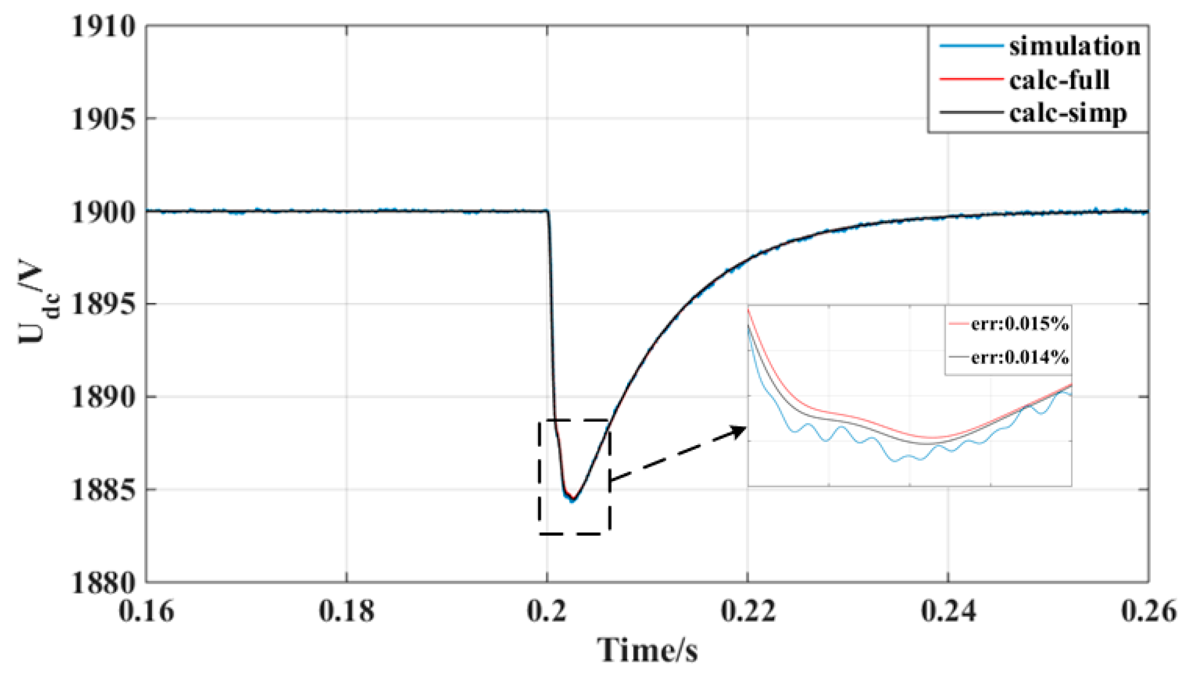
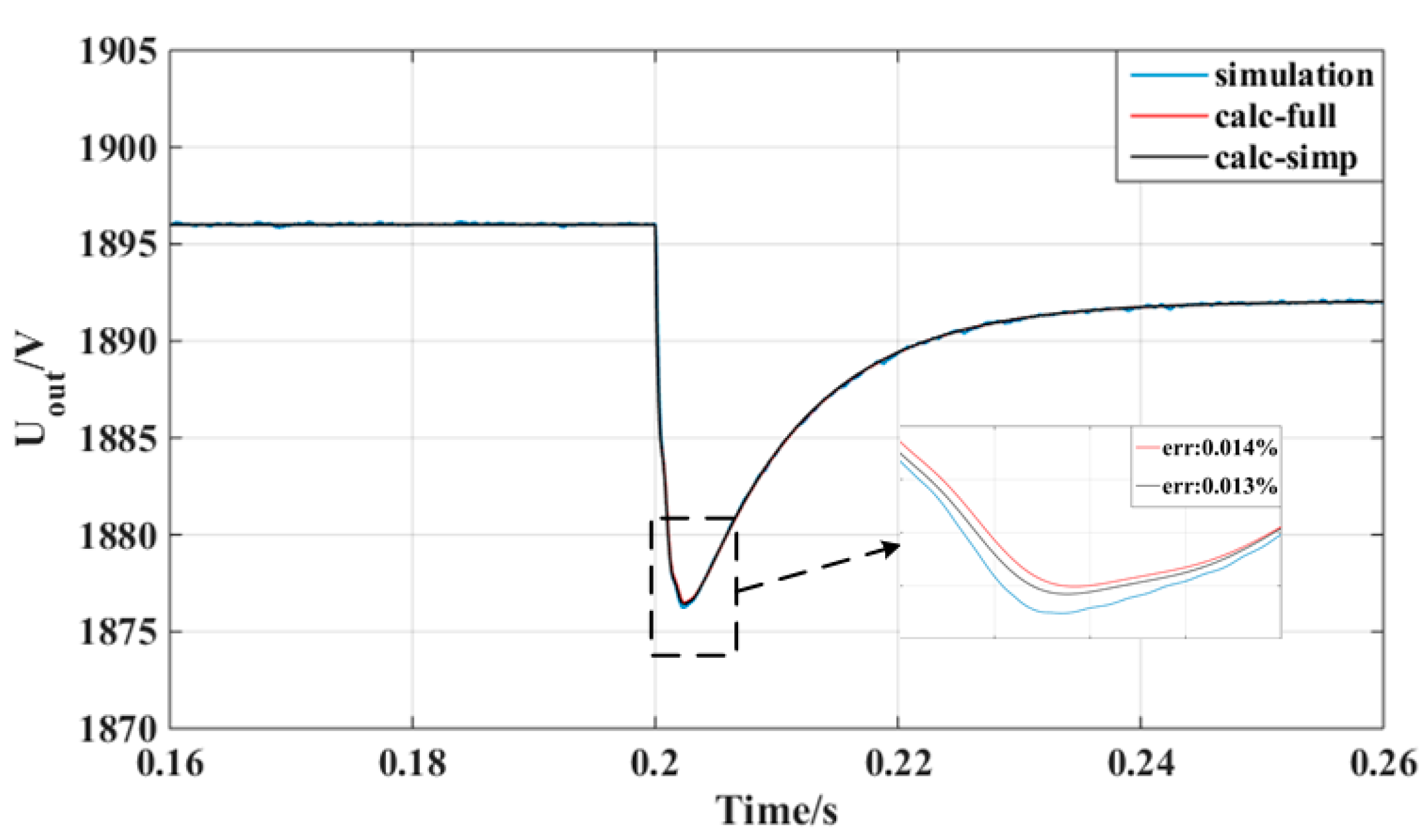
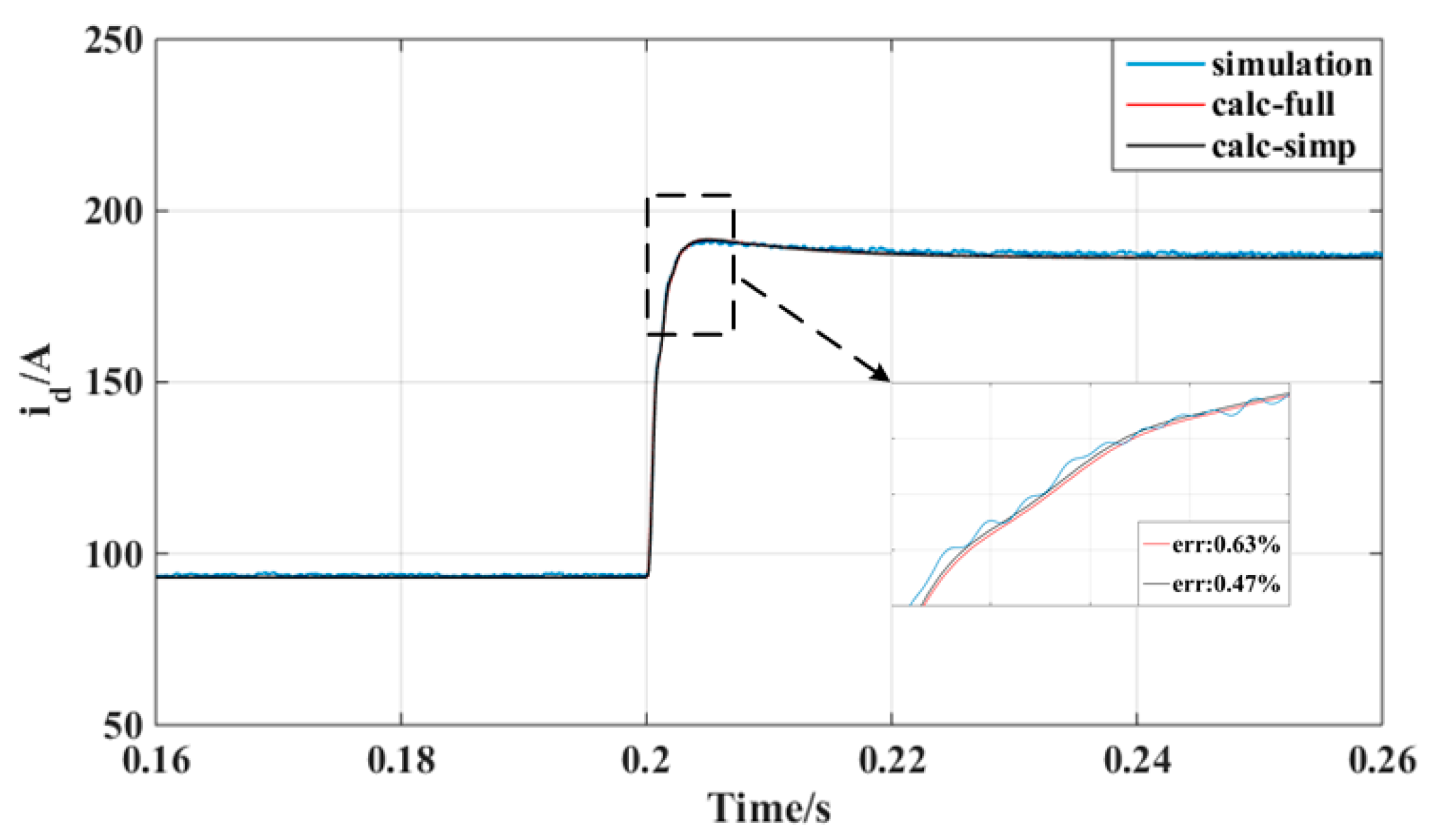
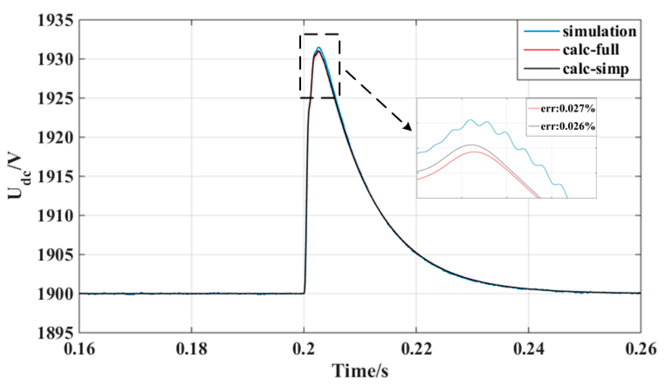
4. Simulation Results

In order to verify the accuracy of the full-order and reduced-order mathematical model analyzed in Section 3, the full-scale simulation of MP-PET has been implemented. The main circuit parameters are presented in Table 2, which were designed based on the actual project.

In this simulation model, the input stage adopts the double-loop decoupling control strategy of the cascaded H-bridge, where the outer loop is the dc bus voltage feedback control loop and the inner loop is the grid current control loop. The isolation stage adopts an open-loop control strategy and the high-frequency voltage is 50% duty cycle square wave.

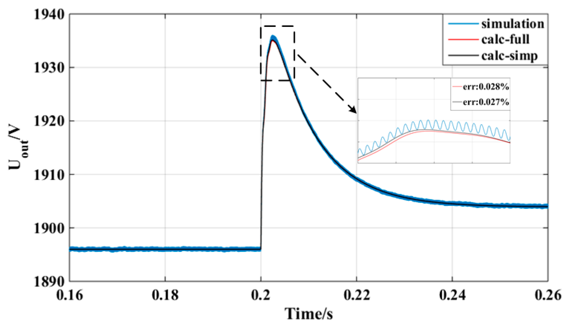
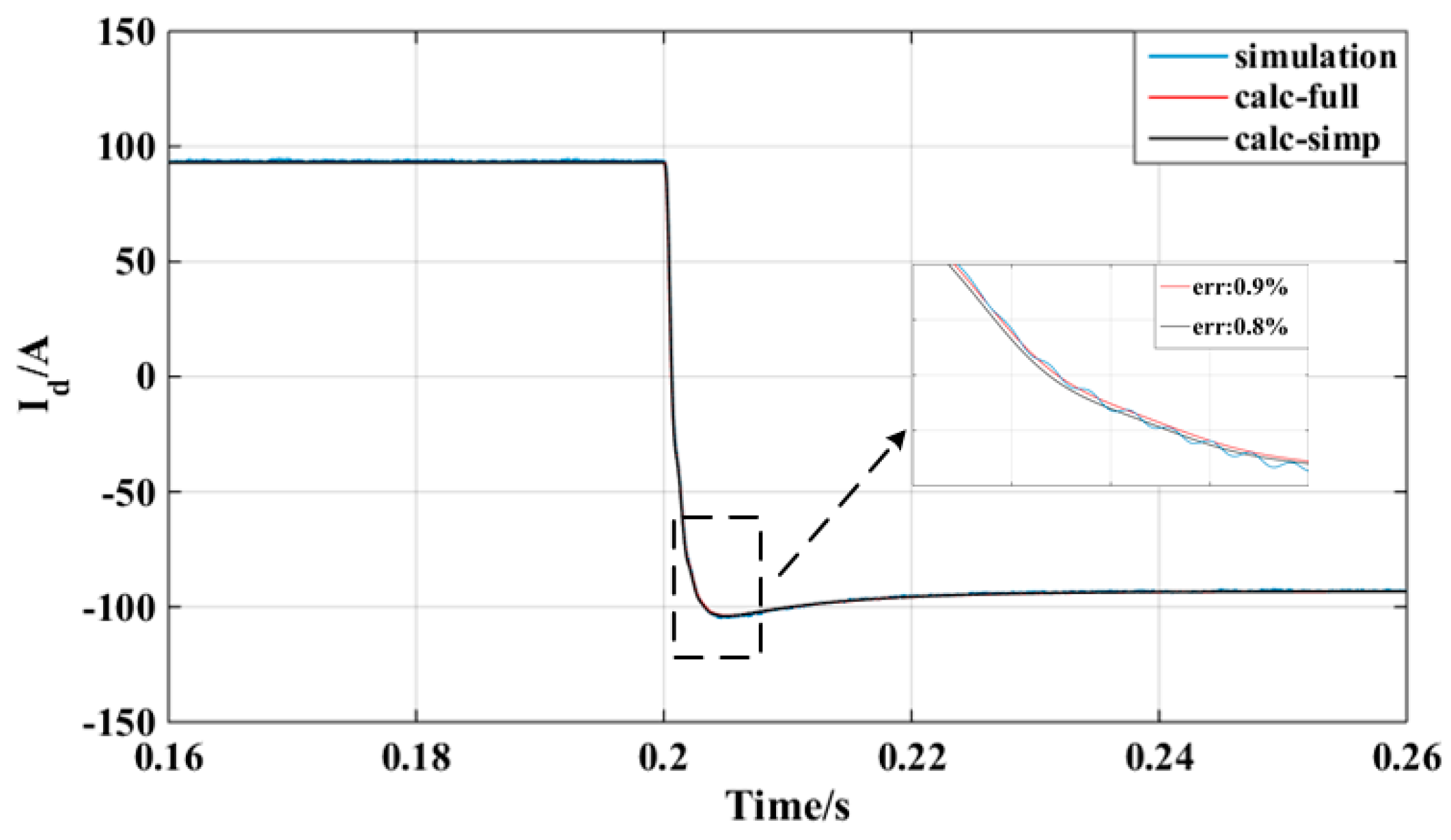
4.1. Case I: Model Verification by Load Step

The MP-PET operates at a rectified state and the grid releases 2.28 MW active power and 0 MW reactive power. Meanwhile, the dc output rating voltage is 1900 V and the active power absorbed by each DAB submodule from the ac network is 76 kW. When the system runs to 0.2 s, the load of the positive converter is raised from 1.14 MW to 2.28 MW and the load of the negative converter is constant.

The calculated results and the simulation results are presented in Figure 5, Figure 6 and Figure 7. When the system runs to 0.2 s, the dc bus voltage and grid current produce a transient fluctuation, which is caused by a load step. Then, each variable begins to enter a steady state and stay near the rating value. Furthermore, it is shown that the reduced-order small signal model and the full-order small signal numerical results have a high consistency with electromagnetic simulation results where err indicates the percentage of the maximum error relative to the simulation result.

4.2. Case II Model Verification by Power Inversion

In this simulation, the MP-PET has the same steady working operation as Case I. When the system runs to 0.2 s, the load of the positive converter is changed from 1.14 MW to −1.14 MW and the load of the negative converter is constant.

Figure 8, Figure 9 and Figure 10 present the results of the dynamic performance on dc bus voltage and grid current, respectively. When the system runs to 0.2 s, the load changes from 1.14 MW to −1.14 MW, which causes transient fluctuation of the system state variables. As shown in the above three figures, the theoretical calculation results are consistent with the simulation results so as to verify the effectiveness of the small signal model proposed by this paper. In the above figures, err represents the percentage of the maximum error relative to the simulation result.

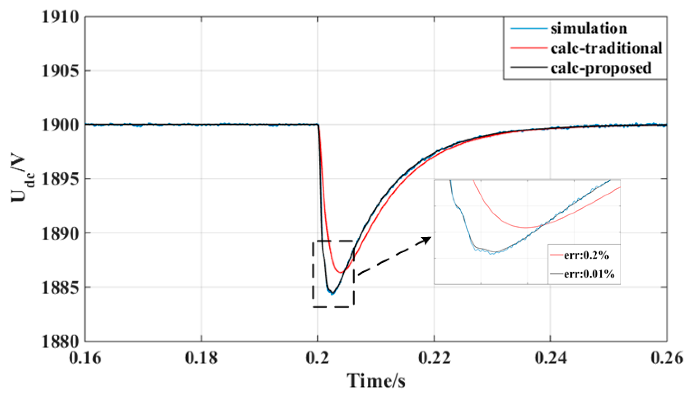
4.3. Case III Model Contrast Verification

In this simulation, the results of the dc bus voltage dynamic performance from the different reduced-order model are presented in Figure 11. In this figure, err stands for the percentage of the maximum error relative to the simulation result.

As shown in Figure 11, because the traditional model is based on the steady-state power balance relationship of the converter, it cannot accurately reflect the dynamic performance of the dc bus voltage. However, compared to the traditional reduced-order model, the proposed reduced-order model constructed by using instantaneous variable theory has higher precision. Therefore, the accuracy of the reduced-order small signal model established by this paper is well verified through simulation.

5. Conclusions

This paper takes MP-PET as the research target to build a full-order small signal mathematical model in the d-q rotating coordinate system by using the state space average method. Furthermore, the model interface between the controller system and converter is provided so as to combine it into one state space equation. Based on the equation, the small signal model is simplified through the eigenvalue participation factor analysis method. It reduces the order of the model by 50%, which greatly reduces the computational complexity of the system. Meanwhile, it can reduce the number of sensors to lower the cost of the system and simplify the complexity of the system controller design under the same effects. Compared with the full-order model, the proposed reduced-order model is accurate enough and simplified, and the validity of the reduced-order small signal model is verified against the electromagnetic transient model. The simulation results show that both the full-order and reduced-order small signal models coincide well with the dynamic performance of the dc bus voltage, which verifies the correctness and effectiveness of the theoretical analysis above.

References

1. Bifaretti, S.; Zanchetta, P.; Watson, A. Advanced power electronic conversion and control system for universal and flexible power management. IEEE Trans. Smart Grid 2011, 2, 231–243. [Google Scholar] [CrossRef]
2. Glinda, M.; Marquardt, R. A new AC/AC multilevel converter family. IEEE Trans. Ind. Electron. 2005, 52, 662–669. [Google Scholar] [CrossRef]
3. Gu, C.; Zheng, Z.; Xu, L. Modeling and control of a multiport power electronic transformer (PET) for electric traction applications. IEEE Trans. Power Electron. 2016, 31, 915–927. [Google Scholar] [CrossRef]
4. Falcones, S.; Ayyanar, R.; Mao, X. A DC-DC multiport-converter-based solid-state transformer integrating distributed generation and storage. IEEE Trans. Power Electron. 2013, 28, 2192–2203. [Google Scholar] [CrossRef]
5. Sabahi, M.; Goharrizi, A.Y.; Hossemi, S.H. Flexible power electronic transformer. IEEE Trans. Power Electron. 2010, 25, 2159–2169. [Google Scholar] [CrossRef]
6. Contreras, J.P.; Ramirez, J.M. Multi-fed power electronic transformer for use in modern distribution systems. IEEE Trans. Smart Grid 2014, 5, 1532–1541. [Google Scholar] [CrossRef]
7. Lu, X.; Lin, W.; Wen, J.; Li, Y. Modularized Small Signal Modeling Method for DC Grid. Proc. CSEE 2016, 36, 2880–2889. [Google Scholar]
8. Yang, J.; Liu, K.; Wang, D.; Qin, L. Small Signal Stability Analysis of VSC-HVDC Applied to Passive Network. Proc. CSEE 2015, 35, 2400–2408. [Google Scholar]
9. Zheng, C.; Zhou, X. Small Signal Dynamic Modeling and Damping Controller Designing for VSC Based HVDC. Proc. CESS 2006, 26, 7–12. [Google Scholar]
10. Adam, G.P.; Ahmed, K.H.; Finney, S.J.; Williams, B.W. Generalized Modeling of DC Grid for Stability Studies. In Proceedings of the 4th International Conference on Power Engineering, Energy and Electrical Drives, Istanbul, Turkey, 13–17 May 2013; pp. 1168–1174. [Google Scholar]
11. Magne, P.; Nahid-Mobarakeh, B.; Pierfederici, S. General Active Global Stabilization of Multiloads DC-Power Networks. IEEE Trans. Power Electron. 2012, 27, 1788–1798. [Google Scholar] [CrossRef]
12. Cole, S.; Beerten, J.; Belmans, R. Generalized dynamic VSC-MTDC model for power system stability studies. IEEE Trans. Power Syst. 2010, 25, 1655–1662. [Google Scholar] [CrossRef]
13. Chaudhuri, N.R.; Majumder, R.; Chaudhuri, B.; Pan, J. Stability analysis of VSC-MTDC grids connected to multimachine AC systems. IEEE Trans. Power Deliv. 2011, 26, 2774–2784. [Google Scholar] [CrossRef]
14. Alsseid, A.M.; Jovcic, D.; Starkey, A. Small signal modelling and stability analysis of multiterminal VSC-HVDC. In Proceedings of the 2011 14th European Conference on Power Electronics and Applications, Birmingham, UK, 30 August–1 September 2011; pp. 1–10. [Google Scholar]
15. She, J.; Zheng, Z.; Ai, Q. Modeling of DC micro-grid and stability analysis. Electr. Power Autom. Equip. 2010, 30, 86–90. [Google Scholar]
16. Liutanakul, P.; Awan, A.-B.; Pierfederici, S.; Nahid-Mobarakeh, B.; Meibody-Tabar, F. Linear stabilization of a DC bus supplying a constant power load: A general design approach. IEEE Trans. Power Electron. 2010, 25, 475–488. [Google Scholar] [CrossRef]
17. Anand, S.; Fernandes, B.G. Reduced-order model and stability analysis of low-voltage DC microgrid. IEEE Trans. Ind. Electron. 2013, 60, 5040–5049. [Google Scholar] [CrossRef]
18. Li, Y.; Tang, G.; Wu, Y.; Yang, J. Modeling, Analysis and Damping Control of DC Grid. Trans. Power Electron. 2017, 37, 3372–3382. [Google Scholar]
19. Li, Z.; Qu, P.; Wang, P. DC Terminal Dynamic Model of Dual Active Bridge Series Resonant Converter. In Proceedings of the 2014 IEEE Conference and Expo Transportation Electrification Asia-Pacific (ITEC Asia-Pacific), Beijing, China, 31 August–3 September 2014; pp. 1–5. [Google Scholar]
20. Pogaku, N.; Prodanović, M.; Green, T.C. Modeling, Analysis and Testing of Autonomous Operation of an Inverter-Based Microgrid. IEEE Trans. Power Electron. 2007, 22, 613–625. [Google Scholar] [CrossRef] [Green Version]
Figure 1. The circuit topology of MP-PET.
Energies 12 02130 g001
Figure 2. The equivalent circuit topology of DAB in the PET.
Energies 12 02130 g002
Figure 3. The diagram of the d-q axis decoupling double closed-loop control strategy.
Energies 12 02130 g003
Figure 4. The eigenvalues spectrum of MP-PET.
Energies 12 02130 g004
Figure 5. The waveform of input dc bus voltage (load step).
Energies 12 02130 g005
Figure 6. The waveform of output dc bus voltage (load step).
Energies 12 02130 g006
Figure 7. The waveform of the grid current peak value (load step).
Energies 12 02130 g007
Figure 8. The waveform of input dc bus voltage (power inversion).
Energies 12 02130 g008
Figure 9. The waveform of output dc bus voltage (power inversion).
Energies 12 02130 g009
Figure 10. The waveform of the grid current peak value (power inversion).
Energies 12 02130 g010
Figure 11. The waveform of input dc bus voltage (contrast model).
Energies 12 02130 g011