Article

Research on Theoretical Calculation Methods of Photovoltaic Power Short-Circuit Current and Influencing Factors of Its Fault Characteristics

1
Yangjiang Power Supply Company, Ltd., Yangjiang 529500, China
2
State Key Laboratory of Advanced Electromagnetic Engineering and Technology, Huazhong University of Science and Technology, Wuhan 430074, China
*
Author to whom correspondence should be addressed.
Energies 2019, 12(2), 316; https://doi.org/10.3390/en12020316
Submission received: 9 December 2018 / Revised: 3 January 2019 / Accepted: 16 January 2019 / Published: 20 January 2019

Abstract

:
With the substantial increase in the capacity of grid-connected photovoltaic (PV) power, the adverse effects of its complex fault characteristics on grid relay protection are increasingly highlighted. Based on the introduction of the topology and the control strategy on low-voltage ride through of PV power, a theoretical solution method for solving the fault current of PV power is proposed by taking account of the DC bus voltage fluctuation, and a theoretical calculation model of its transient and steady state is established. The correctness of the theoretical results is verified by the numerical simulation results and low-voltage ride through (LVRT) experiment results. Furthermore, to gain a better understanding of the factors influencing PV power fault characteristics, the effects of several factors including proportional integral (PI) controller parameters, fault voltage sag depth, and PV power load level on PV power fault characteristics are analyzed by using simple variable method. The obtained results can provide a theoretical reference for the control parameter design and protection research of PV power.

1. Introduction

In recent years, solar power has become an important field for global energy transformation with rapidly increased installed capacity, which is mainly attributed to its technology advancement and cost reduction [1]. In order to prevent the danger of the grid-connected PV power to the safe and stable operation of the power grid during power grid fault, in the relevant regulations for grid-connected operation of PV power, it is clearly required that large and medium-sized PV power stations should possess LVRT capability [2]. As the power generation mode, circuit topology, and LVRT control strategy of PV power is quite unique, its fault characteristics are very different from traditional synchronous motors. With large numbers of PV power sources adopting the LVRT control strategy, the complex short-circuit currents that they feed will have many adverse effects on the relay protection of power grid, which may lead to protection maloperation or refusing action, thus threatening the safe and stable operation of the power system. Therefore, in-depth analysis of the short-circuit current characteristics of PV power and the establishment of a theoretical analytical calculation model for short-circuit currents have important practical significance for accurately evaluating their impact on power grid relay protection and improving protection performance.
In [3,4,5,6,7], the characteristics and calculation methods of the steady-state fault current of PV power have been studied without considering its transient fault characteristics, therefore the conclusions are only applicable to the steady-state short-circuit analysis. In [8], the mathematical model for the fault analysis of inverter interfaced distributed generator (IIDG) has been first established by using single outer voltage loop control strategy, and then the fault analysis method of distribution network including IIDG has been proposed. However, at present, IIDG usually adopts the double loop control strategy with outer voltage loop and inner current loop [9,10], which cannot be directly simplified to single voltage outer loop control strategy for fault characteristic analysis. In the literature [11,12,13], the fault transient-state and steady-state characteristics of PV power have been studied by assuming that the DC bus voltage is constant during a fault. However, when a fault occurs, the output power of PV power will change substantially, and this change will result in the DC bus voltage fluctuation, which eventually affects the output fault current. Therefore, the above approximate analysis method needs further improvement. Meanwhile, since the factors affecting the transient fault characteristics of PV power are not analyzed in the literature [11,12,13], the relationship between these characteristics (such as transient duration, transient peak, transient component frequency, etc.) and the related variables (such as controller parameters, voltage sag depth, load level, etc.) cannot be visually seen. Therefore, it is difficult to apply directly to engineering. To prevent the overvoltage of DC bus caused by unbalanced active power during a fault, the DC bus of PV power is generally equipped with the unloading circuit [14]. In [15,16], the fault transient characteristics of PV power considering the effect of the unloading circuit have been studied by using digital simulation. However, their study is limited to qualitative analysis, and lacks the support of necessary theory analysis.
Aiming to solve the above problems, in this paper, we propose a theoretical solution method and calculation model for analyzing PV power fault transient and steady current by taking account of the DC bus voltage fluctuation and the influence of unloading circuit during fault. The correctness of our model is verified by the digital simulation and LVRT experiment results. Furthermore, the main factors affecting the short-circuit current characteristics of PV power are analyzed based on this model in order to provide the references for relay protection research and controller design of power grids including PV power.

2. PV Power Topology and Its Control Strategy of LVRT

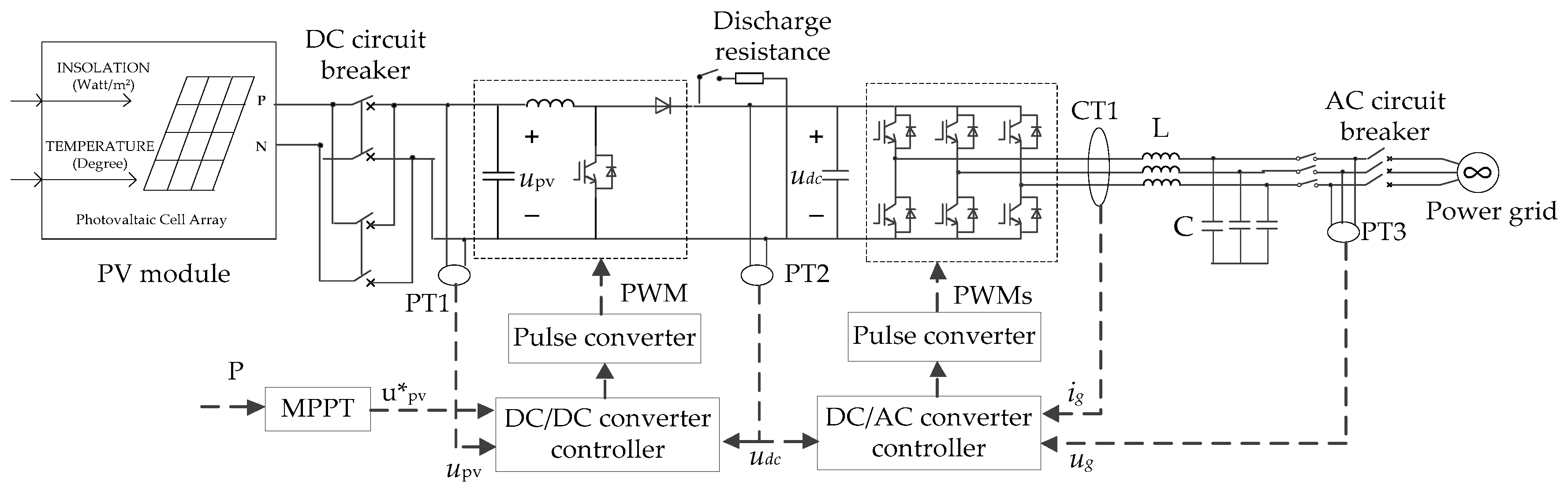
2.1. PV Power Topology and Its Inverter Control Strategy

In general, the inverter topology used in high-power PV power is generally can be either single-stage or double-stage [17]. Among them, the double-stage inverter separates the maximum power point tracking (MPPT) unit [18,19,20] from the grid-connected control unit, which simplifies the design difficulty of the control system, and therefore is more popular in practical applications [17], and the topology of the double-stage inverter is shown in Figure 1. The photovoltaic array generates direct current which is boosted by the DC/DC circuit and then connected to the DC bus, and then connected to the power grid via the DC/AC converter and the filter circuit. In addition to boosting the voltage, the boost converter is used to control the port voltage of PV array tracking the instruction voltage value corresponding to the maximum power point, and physically isolate the port voltage of PV array from the DC bus voltage.
To calculate the output power of photovoltaic power, the vector decoupling control method is usually adopted, which generally directs the grid positive sequence voltage to the d-axis, and the output power equation is
{ P = u g d i g d + u g q i g q = U g i g d Q = u g q i g d u g d i g q = U g i g q
Under normal circumstances, the photovoltaic power operates under unit power factor conditions and adopts the double loop control strategy with outer voltage loop and inner current loop. At this time, in the d and q axis two-phase rotating coordinate system, the inverter control equation is
{ u s d = ( k P + k I / s ) ( i d * i d ) + R i d + ω 1 L i q + u g d u s q = ( k P + k I / s ) ( i q * i q ) + R i q ω 1 L i d + u g q i g d 0 * = ( k vP + k vI / s ) ( u d c * u d c ) i g q 0 * = 0
where superscript * represents the controller instruction value; k vP and k vI is the P and I parameters of outer voltage loop PI controller; k P and k I is the P and I parameters of inner current loop PI controller; i d 0 * and i q 0 * is the d and q axis instruction value of grid current under normal conditions.
In the case of faults, the photovoltaic power should possess LVRT capability [2] in order to meet the reactive power support requirements of the system. At the same time, to ensure that the DC bus voltage still possess a certain degree of adjusting ability during the fault, the outer voltage control loop of photovoltaic power is not blocked during the fault. At this time, LVRT control equation of the photovoltaic power is
{ i g q 1 * = { 0 U T > 0.9 1.5 ( 0.9 U T ) 0.2 U T 0.9 i g max * U T < 0.2 i g d 1 * = min ( i g d 0 * , i g max * i g q 1 * 2 )
where: U T is the positive sequence voltage amplitude on grid side after fault; i g max * is the instruction value of the inverter maximum output current; i g q 1 * and i g d 1 * is the instruction value of d and q axis current after fault.
In addition, in the case of asymmetric faults, PV power generally adopts a balanced (no negative sequence component) output current control strategy based on positive sequence voltage measurement [21]. First, the amplitude and phase of the positive sequence component in the fault voltage are measured by a phase-locked loop (PLL) [22], and the instruction values of the output positive sequence active and reactive current are obtained according to Equation (3). Then, the output current of the photovoltaic power quickly tracks the instruction value based on the inner current loop control link, so the photovoltaic power will not output negative sequence fault currents under the asymmetric fault.

2.2. DC Unloading Circuit Control Strategy

When the voltage sags deeply, the active output of the photovoltaic power is limited, and in a short time after the fault, the output power of the photovoltaic array remains nearly unchanged due to the voltage regulation of the DC/DC circuit. In order to prevent the DC bus voltage from overvoltage caused by the unbalanced active power, a commonly used approach is to add a DC unloading circuit on the DC bus side [14]. The switching control is based on judging whether the DC bus voltage is off-limit or not, and the specific control principle as shown in Figure 2. The switching signal of the unloading circuit is obtained by the DC voltage difference through the PI link and pulse width modulation (PWM) link, which can effectively reduce the fluctuation of the DC side voltage.

3. Analysis of PV Power Fault Characteristics

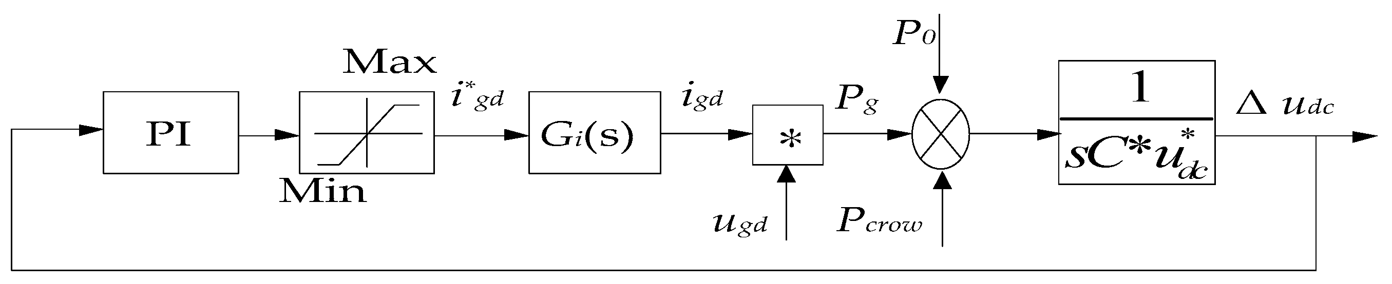
3.1. Fault Current Calculation Model with Considering DC Bus Voltage Fluctuation

3.1.1. Symmetrical Fault Condition

When a fault happens in the grid, the DC bus voltage fluctuates due to power imbalance, which will directly affect the short-circuit current characteristics. According to the characteristics of capacitor energy storage and the principle of energy conservation, the DC bus voltage equation is
u d c 2 = u d c * 2 + 2 C t 0 t ( p 0 p g p c r o w ) d t
where: u d c * is the rated voltage of the DC bus; udc is the DC bus voltage; C is the DC bus capacitor; t0 is the fault occurrence time; p0 is the input active power of the PV array; pg is the output active power of the PV power; pcrow is the consumed power of the DC unloading circuit.
Assuming that Δ u d c is the fault component of the DC bus voltage during the fault, then
u d c = u d c * + Δ u d c
To ensure the safe operation of both the DC bus and the inverter, it is generally specified that the maximum allowable voltage on the DC bus side should not exceed 1.1 p.u [23,24]. At this time, squaring Equation (5), then
u d c 2 u d c * 2 + 2 u d c * Δ u d c
According to the simultaneous equation of Equations (4) and (6), the DC bus fault component voltage equation is
Δ u d c = t 0 t ( p 0 p g p c r o w ) d t C u d c *
Ignoring the power loss of the inverter and filter circuit, the control block diagram of the outer voltage loop of the inverter is shown in Figure 3.
In Figure 3 and Figure 4, the current control inner loop is typically designed as a typical I-type system in order to achieve faster current follow-up characteristics. At the same time, the cutoff frequency is generally less than 1/10 of the equivalent switching frequency [25]. If the equivalent switching frequency is 15,000 Hz, the cutoff frequency is 1000 Hz. At this time, the decay time constant τ = 1 / 2 π f c = 0.16   m s , meaning that the active current can track the active current command within a few milliseconds. The fast tracking of the reactive current can also be proved using the same approach. Therefore, it can be approximated that
{ i g d = i g d * i g q = i g q *
According to the simultaneous equation of Equations (1), (2), (7) and (8), the equation of DC bus fault component voltage can be rewritten as
Δ u d c = 1 C u d c * [ t 0 t p 0 d t t 0 t u g d ( k p Δ u d c + k i 0 t Δ u d c d t ) d t ]
When a short-circuit fault occurs in the power grid, since the fault duration is generally short (depending on the protection action time at the fault location), the external conditions such as the insolation and temperature can be assumed to be constant, then the instruction voltage value corresponding to the maximum power point of the PV array also remains unchanged. When the DC bus voltage fluctuates during the fault period, the booster converter controls the switching by its voltage loop controller, which adjusts its transfer ratio to control the port voltage of the PV array being basically constant as its instruction value, therefore keeping the active output power of the PV array constant during the fault period. Therefore, if the PV array and the booster converter are taken as a whole, they can be equivalent to a constant active power source during the fault period. Doing second order derivative on time to Equation (9), then
D 2 Δ u d c + k p u g d u d c * C D Δ u d c + k i u g d u d c * C Δ u d c = 0
where: D2 is the second-order differential factor; D is the first-order differential factor; ugd is the d-axis voltage on the grid side after the fault, and its value is constant during the fault.
Because the output current is continuous at the moment of fault, namely i g d ( t 0 ) = i g d ( t 0 + ) , the definite conditions of Equation (10) are
{ Δ u d c ( t 0 ) = 0 D Δ u d c ( t 0 ) = P 0 u g d ( t 0 + ) i g d ( t 0 + ) u d c * C = δ P 0 u d c * C
where: δ is the sag depth of the positive sequence voltage.
Equation (10) is a typical second-order constant-coefficient homogeneous differential equation, and its characteristic equation is
λ 2 + k p u g d u d c * C λ + k i u g d u d c * C = 0
Theoretically, the characteristic roots of Equation (12) include two cases of two different real roots and two conjugate complex roots, which are analyzed separately below.
(1) Two different real roots of characteristic Equation (12)
Based on Equations (10) and (11), the analytical expression of the fault component of the DC bus voltage is
Δ u d c ( t ) = C 1 e λ 1 t C 1 e λ 2 t
where t = t t 0 ; σ = u g d / u d c * C ; λ 1 = ( k p σ k p 2 σ 2 4 k i σ ) / 2 ; λ 2 = ( k p σ + k p 2 σ 2 4 k i σ ) / 2 ; C 1 = 2 δ P 0 / u d c * C k p 2 σ 2 4 k i σ .
Substituting the above formula into Equation (3), the output currents of the photovoltaic power d and q-axis are
{ i g d ( t ) = P 0 u g d + C 2 e λ 1 t C 3 e λ 2 t i g q ( t ) = i g q *
where: C 2 = k p C 1 k i C 1 / λ 1 ; C 3 = k p C 1 k i C 1 / λ 2 .
The equation is rewritten in the three-phase coordinate system as
{ i g a ( t ) = C 4 cos ( ω 1 t + φ 1 + θ 1 ) + C 2 e λ 1 t cos ( ω 1 t + φ 1 ) C 3 e λ 2 t cos ( ω 1 t + φ 1 ) i g b ( t ) = C 4 cos ( ω 1 t + φ 1 + θ 1 2 3 π ) + C 2 e λ 1 t cos ( ω 1 t + φ 1 2 3 π ) C 3 e λ 2 t cos ( ω 1 t + φ 1 2 3 π ) i g c ( t ) = C 4 cos ( ω 1 t + φ 1 + θ 1 + 2 3 π ) + C 2 e λ 1 t cos ( ω 1 t + φ 1 + 2 3 π ) C 3 e λ 2 t cos ( ω 1 t + φ 1 2 3 π )
where: φ 1 is the initial phase of A phase current before the fault; θ 1 = arctan [ P 0 / ( u g d i g q * ) ] ; C 4 = ( P 0 / u g d ) 2 + i g q * 2 .
It can be seen from Equations (14) and (15) that when the characteristic equation has two different real roots, the fault current of PV power does not contain the damping DC component, but contains one steady-state fundamental frequency component and two kinds of free fundamental frequency components, which is quite different comparing with the case in conventional synchronous motors. Among them, the initial values and the decay time constants of the two free frequency components are different, and their phases are opposite. The fundamental frequency component with large initial value decays faster, and its phase is opposite to the steady-state component, while the fundamental frequency component with small initial value decays slowly, and its phase is the same as the steady-state component. Based on these analyses, it can be deduced that the d-axis current and the phase current envelope of the PV power will first increase and then decrease during the fault, which will be verified in the subsequent digital simulation and LVRT experiment.
(2) Two conjugate complex roots of characteristic Equation (12). Based on Equations (10) and (11), the analytical expression of the fault component of the DC bus voltage can be obtained as
Δ u d c ( t ) = A 1 e α t sin ( β t )
where: α = k p σ / 2 ; β = 4 k i σ k p 2 σ 2 / 2 ; A 1 = 2 δ P 0 / ( u d c * C 4 k i σ k p 2 σ 2 ) .
{ i g d ( t ) = P 0 u g d + A 2 e α t sin ( β t θ 2 ) i g q ( t ) = i g q *
where: A 2 = A 1 k i / σ ; θ 2 = arctan ( 2 4 k i σ k p 2 σ 2 3 k p σ ) .
The equation is rewritten in the three-phase coordinate system as
{ i g a ( t ) = C 4 cos ( ω 1 t + φ 1 + θ 1 ) + A 3 s i n [ ω 2 t θ 2 + φ 1 ] + A 3 sin [ ω 3 t θ 2 φ 1 ] i g b ( t ) = C 4 cos ( ω 1 t + φ 1 + θ 1 2 3 π ) + A 3 s i n [ ω 2 t θ 2 + φ 1 2 3 π ] + A 3 sin [ ω 3 t θ 2 φ 1 2 3 π ] i g c ( t ) = C 4 cos ( ω 1 t + φ 1 + θ 1 + 2 3 π ) + A 3 s i n [ ω 2 t θ 2 + φ 1 + 2 3 π ] + A 3 sin [ ω 3 t θ 2 φ 1 + 2 3 π ]
where: A 3 = A 2 e α t / 2 ; ω 2 = β + ω 1 ; ω 3 = β ω 1 .
It can be seen from Equations (17) and (18) that when the characteristic equation has two conjugate complex roots, the fault current of the PV power contains one steady-state fundamental frequency component and two kinds of free non-fundamental frequency AC components, without decaying DC component and free fundamental frequency components. Among them, the two free non-baseband AC components possess the same initial values and decay time constant, but with different frequency and phase. The superposition of the two AC components will be a decaying AC component at a fixed frequency. At this time, the d-axis current and the phase current envelope of PV power will first increase and then decay oscillatorily during the fault, which is significantly different from the fault characteristics of traditional synchronous motor.

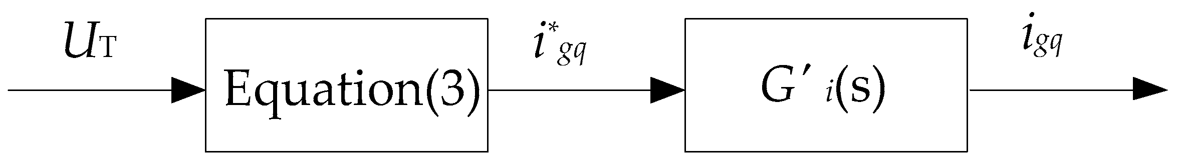
3.1.2. Asymmetric Fault Condition

When the asymmetrical fault occurs, a balanced (no negative-sequence component) output current control strategy is generally used in the inverter of PV power [21], which causes that only the positive-sequence current is generated by PV power. The double-frequency power will be generated due to the existence of the positive-sequence current and the negative-sequence fault voltage. Their relational expression is
{ P g 2 = P g 2 cos cos ( 2 ω 1 t ) + P g 2 sin s i n ( 2 ω 1 t ) Q g 2 = Q g 2 cos cos ( 2 ω 1 t ) + Q g 2 sin s i n ( 2 ω 1 t ) [ P g 2 cos P g 2 sin Q g 2 cos Q g 2 sin ] = [ u g d u g q u + g d u + g q u g q u g d u + g q u + g d u g q u g d u + g q u + g d u g d u g q u + g d u + g q ] [ i + g d i + g q i g d i g q ]
where: All the parameters are expressed by the per-unit value. P g 2 and Q g 2 represent the double-frequency active and reactive power respectively; u + g d and u + g q represent the d-axis and q-axis components of the positive-sequence voltage respectively; u g d and u g q represent the d-axis and q-axis components of the negative-sequence voltage respectively; i + g d and i + g q represent the d-axis and q-axis components of the positive-sequence current respectively; i g d and i g q represent the d-axis and q-axis components of negative-sequence current respectively, whose value is actually 0 due to the control strategy of the negative-sequence fundamental-frequency current restraint.
Affected by the double-frequency active power, the double-frequency voltage fluctuation of the DC bus is generated, which leads to the double-frequency d-axis current through the PI controller link in the outer voltage loop, and it can be deduced from Equation (2). Meanwhile, the q-axis current is not affected by the above process, so the double-frequency q-axis current is still 0. Then, by changing the d,q-axis coordinate system to abc coordinate system, the double-frequency d,q-axis current are transformed into positive-sequence triple-frequency current and negative-sequence fundamental-frequency current in the three-phase current, but the negative-sequence fundamental-frequency current will be restrained [21]. The whole generation mechanism is shown in Figure 5.
It can be seen from Figure 5 that the generated double-frequency power only affects the triple-frequency phase current, which has no effect on the positive-sequence fundamental-frequency phase current, so the method for solving the d,q-axis positive-sequence current is the same as the symmetrical fault’s. It can be known from Equations (14) and (17) that the d-axis positive-sequence steady-state current is P 0 u gd + , q-axis positive-sequence steady-state current is i g q * , and the negative-sequence voltage can also directed to the negative sequence d-axis, which means u g q =0. Then, based on Equation (19), the steady-state double-frequency active power can be solved as
P o 2 = P 0 u gd u gd + cos ( 2 ω 1 t ) i g q * u gd sin ( 2 ω 1 t ) = A 4 cos ( 2 ω 1 t θ 3 )
where: A 4 = ( P 0 u gd u gd + ) 2 + ( i g q * u gd ) 2 ; θ 3 = arctan ( i g q * u gd u gd + P 0 u gd ) .
Furthermore, based on Equation (4), the steady-state DC bus double frequency voltage Δ u d c 2 can be solved as
Δ u d c 2 = A 4 cos ( 2 ω 1 t θ 3 ) 2 C u d c * ω 1
Then based on Equation (2), the steady-state d-axis double-frequency current can be solved as
i g d 2 = k p A 4 cos ( 2 ω 1 t θ 3 ) 2 C u d c * ω 1 k i A 4 s i n ( 2 ω 1 t θ 3 ) 4 C u d c * ω 1 2 = A 5 cos ( 2 ω 1 t θ 4 )
where: A 5 = ( k p A 4 2 C u d c * ω 1 ) 2 + ( k i A 4 4 C u d c * ω 1 2 ) 2 ; θ 4 = arctan ( k i 2 k p ω 1 ) + θ 3 .
Since the double-frequency q-axis current ( i g q 2 ) is 0, the triple-frequency current in abc coordinate system can be solved as
{ i g a ( 3 ) ( t ) = A 5 2 cos ( 3 ω 1 t + φ 1 + θ 4 ) i g b ( 3 ) ( t ) = A 5 2 cos ( 3 ω 1 t + φ 1 + θ 4 2 3 π ) i g c ( 3 ) ( t ) = A 5 2 cos ( 3 ω 1 t + φ 1 + θ 4 + 2 3 π )

3.2. Influences Analysis of Unloading Circuit on Fault Current Characteristics

When the voltage on PV power parallel point is seriously sagged, the DC bus voltage will rise to the limit value within a short time after the fault, triggering the DC unloading circuit startup. However, the output active current of PV power may reach the limit value earlier than the DC unloading circuit startup. Because the time of the DC bus voltage off-limit depends on the speed at which the bus capacitor is charged, and the bus capacitor charging is a physical process with large bus capacitance, the process generally takes several hundred milliseconds or more. The output active current has a fast tracking of its instruction value in milliseconds, and its limit value becomes lower due to the reactive power support requirement of PV power, which can be even lower than the normal running current with the entire over-limit process taking less than tens of milliseconds. After the limit is exceeded, the output active current of PV power will remain at the limit value, namely, the steady state has been reached. Therefore, the startup of the DC unloading circuit actually has no effect on the fault transient characteristics of PV power. This will be verified by subsequent simulation. If a mis-trip of the inverter unloading circuit protection occurs, although the DC bus voltage will continue to rise during the fault period, the output current of the PV power will also reach the steady-state limit after the transient process, which can also be analyzed by the theoretical result developed in this paper. When the output current of PV power reaches the steady-state limit, its characteristics are independent of whether the unloading circuit protection operates or not.

3.3. Steady-State Fault Mathematical Model

Currently, the relay protection is mainly based on the fundamental frequency component of the short-circuit current, in which the steady-state fundamental frequency current dominates. The steady-state fundamental frequency current of PV power will be analyzed in the following two cases where the current does not reach the limit value (non-severe fault) and reaches the limit value (severe fault) respectively.
(1) The current does not reach the limit value
Based on the Equations (14) and (18) in the fault current calculation model, and the control strategy that the output d-axis current of PV power is oriented to the voltage on the parallel point [7], namely, | u g d | = U T , the d-axis and q-axis steady-state value of the fault current and the phase current steady state value can be solved as
{ i g d = P 0 u g d i g q = { 0 | u g d | > 0.9 1.5 ( 0.9 | u g d | ) 0.2 | u g d | 0.9 i φ = i g d 2 + i g q 2 arctan i g d i g q
(2) The current reaches the limit value
At this time, the d-axis value of the fault current will be affected by the limited amplitude. Based on Equation (3), the d-axis and q-axis steady-state value and the phase current steady-state value can be solved as
{ i g d = i g max * 2 i g q 2 i g q = { 1.5 ( 0.9 | u g d | ) 0.2 | u g d | 0.9 i g max * | u g d | < 0.2 i φ = i g max * arctan i g d i g q
It can be seen from the above analytical expression that the amplitude and phase of the fundamental frequency steady-state current of PV power mainly depend on the depth of voltage sag and the load level before the fault. A shallower voltage sag and lighter load results in a smaller amplitude of fundamental frequency steady-state current, while a deeper voltage sag and heavier load leads to a larger amplitude of fundamental frequency steady-state current. The phase angle of the fundamental frequency steady-state current exhibits a large fluctuation range (0° to 90° variation). The lighter the load, the deeper the voltage sag after the fault, the larger the phase angle (up to 90°); the smaller the voltage sag, and the larger the active output before the fault, the lower the phase angle of the fundamental wave (the minimum value is 0°). The analytical expression also shows that in the short-circuit current calculation, when the current does not reach the limit value during the fault, PV power can be regarded as a voltage-controlled current source model with both amplitude and phase controlled. When the current reaches the limit value, it can be regarded as a voltage-controlled current source model with only phase-controlled in the short-circuit calculation.

4. Simulation and Experiment Verification of PV Power Fault Characteristics

In the third section, the main equations of the theoretical analysis results are Equations (13), (16), (21); (14), (17), (22); and (15), (18), (23), which respectively corresponds to the calculation expressions of the DC bus voltage fault component, d,q-axis current components in the d,q-axis coordinate system, and the three-phase short-circuit current in the abc coordinate system. In this section, to verify the correctness of the above theoretical research about PV power fault characteristics, a digital simulation and LVRT experiment of PV power are carried out, and then the simulation results, experimental results and theoretical calculation results corresponding to the electric variables solved by the above Equations (13)–(18), (21)–(23) are analyzed and compared. See below for details.

4.1. Digital Simulation Verification

In this paper, a system model with PV power is built based on the PSCAD/EMTDC simulation platform (4.5.0.0, Manitoba HVDC Research Centre, Manitoba, Canada) in order to verify the correctness of the above theoretical analysis, as shown in Figure 6. Among them, the rated power of PV array is 0.6 MW, the actual input power is 0.55 MW, the rated voltage on the AC side is 0.69 kV, the rated voltage of the DC bus is 1000 V, the output current limit is 1.2 p.u., and the DC bus voltage limit is 1.1 p.u., DC bus capacitance is 8 mF, unloading circuit resistance is 15 Ω [17], the filter resistance is 0.5 mΩ, and filter inductance is 0.011 mH. Lines AB and BC are 2 km and 1.6 km long respectively. The fault occurred at 2 seconds.
It can be seen from Equation (12) that the analytical solution form of the fault current is related to the PI adjustment parameter, the DC capacitance value and so on. In the actual simulation, the two parameter sets which respectively are kp = 3, ki = 50 and kp = 3, ki = 200 are selected as PI controller parameters for the verification. Among them, the former set represents the case where two different real roots exist in the Formula (12), and the latter set represents the case where two conjugate complex roots exist in the Formula (12). At the same time, the fault characteristics of PV power under the two states where DC unloading circuit starts or not are simulated respectively.

4.1.1. DC Unloading Circuit Does Not Start

First, the simulation where the voltage on the grid parallel point sags to 85% under symmetrical fault is carried out as an example. The waveforms of the three-phase voltage and d,q-axis voltage on the PV power side are shown in Figure 7. In this condition, the unloading circuit does not start. When kp = 3, ki = 50, the theoretical analysis shows that there are two different real roots in Equation (12). The waveforms of DC bus voltage fault component and phase-A output current are shown in Figure 8. Figure 9 shows the waveforms of output d,q-axis current. Among them, the dotted line (subscript th) represents the theoretical calculation waveform, the solid line (subscript sim) represents the simulated waveform.
It can be seen from Figure 9 that during the fault transient process, the output d-axis current rises first rapidly and then gradually decays to a steady state, and no oscillation occurs during the rise and decay. This indicates that the transient component only contains the attenuated DC component, which is consistent with the theoretical Expression (14). The output q-axis current quickly rises to the instruction value of 0.075 p.u. in a short time after the fault occurs, consistent with the foregoing analysis. It can be seen from Figure 8 that the DC bus voltage rises firstly in a short time because the input active power of the inverter is greater than the output active power. As the output d-axis active current of the inverter rises, the output power of the inverter becomes greater than the input power of the photovoltaic array, and the DC bus voltage gradually falls back to a stable value under the control of the voltage outer loop. The theoretical curve agrees well with simulation curve during the whole process, which verifies the correctness of the theoretical analytical model.
When kp = 3, ki = 200, there will be two conjugate complex roots in Equation (12). The waveforms of DC bus voltage fault component and phase-A output current are shown in Figure 10. Figure 11 shows the waveform of d,q-axis output current. Among them, the dotted line (subscript th) represents the theoretical calculation waveform, the solid line (subscript sim) represents the simulated waveform.
It can be seen from Figure 10 that in this case, the output d-axis current oscillates during the decay process, indicating that the transient component contains the decaying AC component, which is consistent with the theoretical Equation (18). It can be seen from Figure 11 that during the process when the DC bus voltage falls back to the stable value, the oscillation condition also occurs due to the interaction of the DC bus voltage with the output current. The theoretical curve and simulation curve of the whole process are also basically consistent, which verifies the correctness of the theoretical analytical model.

4.1.2. DC Unloading Circuit Starts

The simulation where the voltage on the grid parallel point sags to 70% under symmetrical fault is carried out as an example, and the unloading circuit starts after the fault. The waveforms of the three-phase voltage on the PV power side and the output A phase current are shown in Figure 12. When kp = 3, ki = 50, the waveform of the output d,q-axis current is shown in Figure 13. Among them, the dotted line (subscript th) represents the theoretical calculation waveform, the solid line (subscript sim) represents the simulated waveform.
It can be seen from Figure 13 that when the voltage on the parallel point sags deeply, the output d-axis current remains stable after rising to 1.16 p.u. (phase current rises to 1.2 p.u.) due to the output current limit (1.2 p.u.), and the theoretical curve is consistent with the simulation curve, indicating that the theoretical method is still suitable for the analysis of its fault process when the current limit is applied. The output q-axis current quickly rises to the instruction value of 0.28 p.u. in a short time after the fault occurs, which is the same as the theoretical calculation. It can be seen from Figure 12 that the output phase current of PV power rises to the limit value of 1.2 p.u. and then enters a steady-state, and the theoretical curve also agrees well with the simulation curve.

4.1.3. Asymmetric Fault

The simulation where the positive-sequence voltage on the parallel point sags to 85% and the negative-sequence voltage rises to 0.15 p.u. under AB phase-to-phase fault is carried out as an example without the start of the unloading circuit. Among them, the negative sequence voltage is also directed to the d-axis. The waveforms of the three-phase voltage and positive, negative sequence d,q-axis voltage on the PV power side are shown in Figure 14. When kp = 3, ki = 50, the waveforms of output d-axis current and the A-phase output current are shown in Figure 15.
It can be seen from Figure 15a that the d-axis DC current rises to 1.07 p.u. after the fault, and the d-axis steady-state current contains the frequency-doubled AC component with an amplitude of about 0.04 p.u., which is much less than the DC component. In Figure 15b, due to the few triple frequency components in the phase steady current, the phase steady current is still basically a 50 Hz sine wave. In Figure 15, the theoretical curve agrees well with simulation curve during the steady-state period, which verifies the correctness of the theoretical analytical model under the asymmetric fault.

4.2. LVRT Experiment Verification

In this section, the LVRT experiment using a Huawei SUN2000-(33KTL-40KTL) PV inverter is carried out in cooperation with Huawei Technologies Co., Ltd. (Shenzhen, China), and experimental data is analyzed and mapped by using CAAP2008X fault wave-recorder software. The internal structure of PV inverter is shown in Figure 16, and its basic electrical parameters are shown in Table 1.
In Table 1, the sampling frequency 3.2 kHz is the sampling frequency of the control system sampling the electrical signal. In the experiment system, the switching frequency is the same as the sampling frequency.
When a short circuit fault happens in the power system, the dynamic reactive current IT injected into the grid by the Huawei SUN2000 PV inverter should meet the following requirements:
{ I T 0 U T > 0.9 I T 1.5 ( 0.9 U T ) 0.2 U T 0.9 I T 1.05 I N U T < 0.2
In the LVRT experiment of PV inverter, the inverter outlet voltage is the rated value under the normal circumstance. Assuming that the AC phases earth short circuit happens at 0.625 s (corresponding to time 0 in the fault wave-recorder graph), the positive sequence voltage at the inverter outlet drops to 0.88 p.u., and the experimental wave-recorder graph is shown in Figure 17a. Among them, the N11M, N22M and N33M channels respectively represent the A phase, B phase and C phase voltage at the inverter outlet, whose units are kV. The CRT1M, CRT2M, and CRT3M channels respectively represent the inverter A phase, B phase and C phase current, whose units are kA. Pac7 channel represents the active output power of the inverter monitored through a delay link, whose unit is MW. The FREC channel represents the output frequency of the inverter, whose unit is Hz. Then, the ABC three-phase current is put into one channel in the wave-recorder software, and the waveform of the wave-recorder is shown in Figure 17b.
It can be seen from Figure 17b that the three-phase output current generated by Huawei PV inverter in the case of the asymmetric fault is still symmetrical, indicating that its control strategy under the asymmetric fault is also balanced output current (no negative sequence current) control, which is consistent with the assumption of the aforementioned theoretical analysis.
In this paper, the relevant experimental data is obtained by using the .cfg prefix file and the .data data file in the experimental wave-recorder file, and the data processing is performed on the MATLAB software platform, generating the waves of d-axis output current and q-axis output current which respectively represent output active power and reactive power. Meanwhile, a simulation model is built again on PSCAD/EMTDC software platform, referring to the parameters of Huawei SUN2000 inverter, and its fault time and fault condition are set the same as the experiment, so the relevant simulation waveforms are obtained. Then based on the theoretical analysis in the third section, the theoretical analytical solution and theoretical waveform of the fault current are calculated. Finally, the experimental waveforms, simulation waveforms and theoretical waveforms of the three kinds of current (d-axis current, q-axis current and phase A current) are shown in Figure 18 and Figure 19. Among them, the dotted line (subscript th) represents the theoretical calculation waveform, the solid line (subscript sim) represents the simulated waveform, and the solid line (subscript exp) represents the experimental waveform.
It can be seen from Figure 18 that the d-axis output current generated by Huawei SUN2000 PV inverter rises rapidly first, then gradually oscillates to a stable state in the case of an asymmetrical fault, and the q-axis output current rises to the instruction value quickly within a short time after the fault occurs. In Figure 19, the A-phase output current generated by Huawei PV inverter also shows a trend of increasing gradually and then decreasing, which is obviously different from the fault characteristics of the conventional synchronous motor.
During the whole fault process, the experimental waveforms of the three kinds of current (d-axis, q-axis, and A-phase output current) agree well with the simulation waveform and the theoretical calculation waveform, which further verifies the correctness of the theoretical analytical model.

5. Analysis of Factors Affecting PV Power Characteristics

It can be seen from the above analysis that the fault characteristics of PV power are related to the PI controller parameters, the fault voltage sag depth, and the PV power load level under the given DC bus capacitance and rated voltage. The following part will analyze the impact of each parameter based on a single variable method.

5.1. PI Controller Parameters

The following selects ten fault conditions with 10 different PI controller parameters (Reference [5,6,7,8,9,10,11,12,13]), and with the remaining influencing factors unchanged. Among them, the root mean square (RMS) of the rated line voltage on the parallel point is 690 V, the RMS of the line voltage on the parallel point after the fault is 317 V (0.46 p.u.), the rated power of the PV array is 0.6 MW, the input power is 0.15 MW (0.25 p.u.), and the rated voltage of the DC bus is 1000 V, DC bus capacitance is 8000 uF. The calculation results of the fault characteristic index are shown in Table 2.
In the above table, the free component frequency respectively is the fundamental frequency and the non-fundamental frequencies under the two fault current state solutions (Section 3.1). The decay time constant is non-single and single under the two fault current state solutions, and the transient duration is mainly determined by the longer decay time constant.
It can be seen from Table 2 that as for the free component frequency, only when the proportional adjustment parameter kp takes a small value or the integral adjustment parameter Ki takes a large value, the free component frequency will be far from the fundamental frequency. When the kp and ki parameters are within a certain range, the free component frequency will be either the fundamental frequency or close to the fundamental frequency.
As for the decay time constant, when the free component frequency is not the fundamental frequency, with the increase of the proportional adjustment parameter kp, the free component attenuation accelerates and the transient process shortens, and the integral adjustment parameter ki has little effect on the decay time constant. When the free component is the fundamental frequency, considering that the transient duration is mainly determined by the free component of the slow decay rate, it can be found that as the proportional adjustment parameter kp increases, the transient duration becomes longer, and as the integral adjustment parameter ki increases, the transient duration becomes shorter.
As for the free component peak, when the free component frequency is the fundamental frequency, the free fundamental frequency component of PV power will increase, different from the free fundamental frequency component of the conventional synchronous motor which will decay in this case. This is because among the two free fundamental frequency components, the free component with larger amplitude possesses a phase opposite to the steady-state fundamental frequency component, and the free component with smaller amplitude has the same phase as the steady-state component. Furthermore, the free component peak gradually decreases with the increase of the proportional adjustment parameter kp, but steadily increases with the increase of the integral adjustment parameter ki. On the contrary, when the free component frequency is not the fundamental frequency, the free component peak gradually increases with the increase of the proportional adjustment parameter kp, but gradually decreases with the increase of the integral adjustment parameter ki. The PI regulation parameters show no effect on the steady state value of PV power fault current.

5.2. Fault Voltage Sag Depth

The following selects six fault conditions with six different fault voltage sag depths, and with the remaining influencing factors unchanged. Among them, PI controller parameters kp = 3, ki = 200, PV array rated power is 0.6 MW, input power is 0.15 MW (0.25 p.u.), DC bus rated voltage is 1000 V, DC bus capacitance is 8000 uF. The calculation results of PV power fault characteristic index are shown in Table 3.
It can be seen from Table 3 that when the free component frequency is not fundamental frequency, the deeper the voltage sags, the closer the free component frequency is to the fundamental frequency, and the greater the decay time constant. When the fault current does not reach the limit value, a larger decay time constant means a longer transient time. However, when the fault current reaches the limit value, the transient duration depends mainly on the speed at which the fault current rises to the limit value. The transient duration has little relationship with the decay time constant and is significantly shorter than that in the case where fault current does not reach the limit value.
As for the free component peak, as the fault voltage sags deeper, the greater the free component amplitude, and the greater the fault current steady state value until the limit value is reached.

5.3. Power Load Level

The following selects six fault conditions with six different input power of PV arrays, and with the remaining influencing factors unchanged. Among them, the RMS of the rated line voltage on the parallel point is 690 V (1.0 p.u.), the RMS of the voltage line voltage on parallel point after fault is 317 V (0.46 pu), the PI controller parameter kp = 2, ki = 200, the rated voltage of the DC bus is 1000 V, and the DC bus capacitor is 8000 uF. The calculation results of PV power failure characteristic index are shown in Table 4.
It can be seen from Table 4 that the free component frequency and the decay time constant are independent of the PV power load level. However, with the increase of the PV power load, the free component peak gradually increases in proportion to the load increase, and the steady state value of the fault current continuously increases until the limit value is reached.

6. Conclusions

In order to comprehensively analyze the fault characteristic of PV power and its influencing factors, this paper proposes an analytic method and calculation model for the fault current of PV power by taking account of the DC bus voltage fluctuation during fault. The correctness of the method is verified by the simulation and experiment results, and the main factors affecting the fault current characteristics are analyzed, and the conclusions obtained are as follows:
(1) The structural parameters and control parameters of PV power will affect the fault transient characteristics. The fault current may contain the free component of fundamental frequency or free component of non-fundamental frequency under different parameter design, and their fault characteristics are quite different. When there are two different real roots in the characteristic equation, the fault current transient component of PV power is composed of two kinds of attenuated fundamental frequency components, and their initial value and decay time constant are different, but their phases are opposite. When there are two conjugate complex roots in the characteristic equation, the fault current transient component is composed of two kinds of attenuated free non-fundamental components with same initial value and the decay time constant but different frequency and phase.
(2) As the fault voltage sags deeper and the PV power load increases greater, the larger the peak value of the fault current, the more severe the transient fluctuation. The PI controller parameter largely affects the frequency of the free component. When the proportional controller parameter kp takes a small value or the integral controller parameter ki takes a large value, the free component frequency will be far from the fundamental frequency. When the PI controller parameter refers to the value in a certain range in Table 1, the free component frequency will be the fundamental frequency, and the peak of the free component will be small, with the whole transient process approaching a smooth state.
(3) When the fault voltage sags deeply, the start time of the DC unloading circuit will be later than the time when the output current reaches the limit value. Therefore, if the DC unloading circuit starts, it means that the output current has already reached the limit value. As a result, the DC unloading circuit and current limiting only affect the steady state of the fault current, but show no effect on the transient process.
(4) The amplitude and phase of the steady-state fundamental-frequency component of PV power mainly depend on the depth of voltage sag and the load level before the fault. The deeper the voltage sag, the greater the load, then the larger the fundamental-frequency component amplitude. The phase angle of fundamental-frequency component presents a large fluctuation range. The smaller the load, the deeper the voltage sag after the fault, then the greater the phase angle.
(5) In the calculation of steady-state short-circuit current, the inverter-type power can be equivalent to a voltage-controlled current source. At the same time, when the current does not reach the limit value during the fault, the inverter-type power can be regarded as a voltage-controlled current source model whose amplitude and phase are controlled in the short-circuit calculation. When the current reaches the limit value, the inverter-type power can be regarded as a voltage-controlled current source model whose phase is controlled in the short-circuit calculation.
The above conclusions can provide a reference for relay protection performance evaluation, setting calculation and inverter control parameter design.

Author Contributions

All authors (H.L., K.X., Z.Z., W.L. and A.J.) contributed to compiling the manuscript in its current state. Their contributions included a detailed survey of the literature and state-of-the-art scenarios which were essential for the completion of this paper. H.L. wrote the paper.

Funding

This research was funded by [the Science and Technology Project of China Southern Power Grid Company Limited] grant number [No. 031700KK52160004].

Conflicts of Interest

The authors declare no conflict of interest.

References

  1. Guerrero, J.; Blaabjerg, F.; Zhelev, T.; Hemmes, K.; Monmasson, E.; Jemei, S.; Comech, M.; Granadino, R.; Frau, J. Distributed Generation: Toward a New Energy Paradigm. IEEE Ind. Electron. Mag. 2010, 4, 52–64. [Google Scholar] [CrossRef]
  2. IEEE P1547 Std. IEEE Standard for Distributed Resources Interconnected with Electric Power Systems; IEEE: Piscataway, NJ, USA, 2004. [Google Scholar]
  3. Plet, C.A.; Brucoli, M.; McDonald, J.D.F.; Green, T.C. Fault models of inverter-interfaced distributed generators: Experimental verification and application to fault analysis. In Proceedings of the IEEE Power and Energy Society General Meeting, Detroit, MI, USA, 24–29 July 2011. [Google Scholar]
  4. Li, Z.; Lu, J.; Zhu, Y.; Jiang, W. Ground-Fault Characteristic Analysis of Grid-Connected Photovoltaic Stations with Neutral Grounding Resistance. Energies 2017, 10, 1910. [Google Scholar] [CrossRef]
  5. Haj-ahmed, M.A.; Illindala, M.S. The Influence of Inverter-Based DGs and Their Controllers on Distribution Network Protection. IEEE Trans. Ind. Appl. 2014, 50, 2928–2937. [Google Scholar] [CrossRef]
  6. Zhou, N.; Ye, L.; Wang, Q. Asymmetric Short-circuit Current Calculation for Inverter Interfaced Distributed Generators With Negative Sequence Current Injection Integrated in Power Systems. Proc. CSEE 2013, 33, 41–49. [Google Scholar]
  7. Jia, K.; Gu, C.; Xuan, Z.; Li, L.; Lin, Y. Fault Characteristics Analysis and Line Protection Design Within a Large-Scale Photovoltaic Power Plant. IEEE Trans. Smart Grid 2018, 9, 4099–4108. [Google Scholar] [CrossRef]
  8. Baran, M.E.; El-Markaby, I. Fault Analysis on Distribution Feeders with Distributed Generators. IEEE Trans. Power Syst. 2005, 20, 1757–1764. [Google Scholar] [CrossRef]
  9. Lee, C.; Hsu, C.; Cheng, P. A Low-Voltage Ride-Through Technique for Grid-Connected Converters of Distributed Energy Resources. IEEE Trans. Ind. Appl. 2011, 47, 1821–1832. [Google Scholar] [CrossRef]
  10. Yazdani, A.; Dash, P.P. A Control Methodology and Characterization of Dynamics for a Photovoltaic (PV) System Interfaced with a Distribution Network. IEEE Trans. Power Deliv. 2009, 24, 1538–1551. [Google Scholar] [CrossRef]
  11. Kong, X.; Zhang, Z.; Yin, X. Fault Current Study of Inverter Interfaced Distributed Generators. Distrib. Gener. Altern. Energy J. 2015, 30, 6–26. [Google Scholar] [CrossRef]
  12. Luming, G.; Linan, Q.; Lingzhi, Z.; Ning, C. Impact of fault-ride-through strategy on dynamic characteristics of photovoltaic power plant. J. Eng. 2017, 13, 2130–2134. [Google Scholar] [CrossRef]
  13. Guo, W.; Mu, L.; Zhang, X. Fault Models of Inverter-Interfaced Distributed Generators Within a Low-Voltage Microgrid. IEEE Trans. Power Deliv. 2017, 32, 453–461. [Google Scholar] [CrossRef]
  14. Hansen, A.D.; Michalke, G. Multi-pole permanent magnet synchronous generator wind turbines’ grid support capability in uninterrupted operation during grid faults. IET Renew. Power Gen. 2009, 3, 333–348. [Google Scholar] [CrossRef]
  15. Li, B.; Zhang, H.; Duan, Z. Analysis of the Effect of Control Strategy on the Fault Transient Characteristics of Inverter-based Distributed Generators. Proc. CSU-EPSA 2014, 26, 1–7. [Google Scholar]
  16. Bi, T.; Liu, S.; Xue, A. Fault Characteristics of Inverter-interfaced Renewable Energy Sources. Proc. CSEE 2013, 33, 165–171. [Google Scholar]
  17. Wang, Y.; Ren, B. Fault Ride-Through Enhancement for Grid-Tied PV Systems with Robust Control. IEEE Trans. Ind. Electron. 2018, 65, 2302–2312. [Google Scholar] [CrossRef]
  18. De Brito, M.A.G.; Galotto, L.; Sampaio, L.P.; E Melo, G.D.A.; Canesin, C.A. Evaluation of the Main MPPT Techniques for Photovoltaic Applications. IEEE Trans. Ind. Electron. 2013, 60, 1156–1167. [Google Scholar] [CrossRef]
  19. Pradhan, R.; Subudhi, B. Double Integral Sliding Mode MPPT Control of a Photovoltaic System. IEEE Trans. Contr. Syst. Technol. 2016, 24, 285–292. [Google Scholar] [CrossRef]
  20. Esram, T.; Chapman, P.L. Comparison of Photovoltaic Array Maximum Power Point Tracking Techniques. IEEE Trans. Energy Conver. 2007, 22, 439–449. [Google Scholar] [CrossRef] [Green Version]
  21. Timbus, A.V. Control strategies for distributed power generation systems operating on faulty grid. In Proceedings of the IEEE International Symposium on Industrial Electronics, Montreal, QC, Canada, 9–13 July 2006. [Google Scholar]
  22. Guo, X.; Wu, W.; Chen, Z. Multiple-Complex Coefficient-Filter-Based Phase-Locked Loop and Synchronization Technique for Three-Phase Grid-Interfaced Converters in Distributed Utility Networks. IEEE Trans. Ind. Electron. 2011, 58, 1194–1204. [Google Scholar] [CrossRef]
  23. Abbey, C.; Joos, G. Supercapacitor Energy Storage for Wind Energy Applications. IEEE T. Ind. Appl. 2007, 43, 769–776. [Google Scholar] [CrossRef]
  24. Liang, H.; Feng, Y.; Liu, Z. Research on low voltage ride through of photovoltaic plant based on deadbeat control. Power Syst. Protect. Control 2013, 41, 110–115. [Google Scholar]
  25. Erickson, R.W.; Maksimovic, D. Fundamentals of Power Electronics, 2nd ed.; Springer: New York, NY, USA, 2012; pp. 337–341. [Google Scholar]
Figure 1. Topology of photovoltaic (PV) power.
Energies 12 00316 g001
Figure 2. Control principle of relieving circuit on dc bus side.
Energies 12 00316 g002
Figure 3. Control block diagram of inverter of the external d-axis voltage loop.
Energies 12 00316 g003
Figure 4. Control block diagram of inverter of the external q-axis voltage external loop.
Energies 12 00316 g004
Figure 5. Generation mechanism of positive-sequence triple-frequency current.
Energies 12 00316 g005
Figure 6. Simulation model of Large power grid including PV power.
Energies 12 00316 g006
Figure 7. (a) Waveforms of three-phase voltage. (b) Waveforms of d,q-axis voltage.
Energies 12 00316 g007
Figure 8. (a) Waveforms of bus voltage fault component. (b) Waveforms of phase-A output current.
Energies 12 00316 g008
Figure 9. (a) Waveforms of d-axis output current. (b) Waveforms of q-axis output current.
Energies 12 00316 g009
Figure 10. (a) Waveforms of bus voltage fault component. (b) Waveforms of phase-A output current.
Energies 12 00316 g010
Figure 11. (a) Waveforms of d-axis output current. (b) Waveforms of q-axis output current.
Energies 12 00316 g011
Figure 12. (a) Waveforms of three-phase voltage. (b) Waveforms of phase-A output current when unloading circuit starts.
Energies 12 00316 g012
Figure 13. (a) Waveforms of d-axis output current. (b) Waveforms of q-axis output current.
Energies 12 00316 g013
Figure 14. (a) Waveform of three-phase voltage. (b) Waveform of positive, negative sequence d,q-axis voltage.
Energies 12 00316 g014
Figure 15. (a) Waveform of d-axis output current in phase to phase short circuit fault. (b) Waveform of phase-A current in phase to phase short circuit fault.
Energies 12 00316 g015
Figure 16. Internal structure diagram of Huawei SUN2000 PV inverter.
Energies 12 00316 g016
Figure 17. (a) Wave-recorder graph of the low-voltage ride through (LVRT) experiment. (b) Wave-recorder graph of three-phase output current.
Energies 12 00316 g017
Figure 18. (a) Waveforms of d-axis output current. (b) Waveforms of q-axis output current.
Energies 12 00316 g018
Figure 19. Waveforms of phase-A output current.
Energies 12 00316 g019
Table 1. Electrical parameters of Huawei SUN2000 PV inverter.
NameValueNameValue
Maximum DC voltage1000 VIsolating transformer315 V/10 kV
Power output500k WBusbar parasitic inductance20 nH
Voltage output315 VGrid frequency50 Hz
FilterL = 0.15 mH
C = 200 uF
Sampling frequency3.2 kHz
DC capacitance36 × 420 uFGrid equivalent impedance3.8895 mH
Table 2. Influence of proportional integral (PI) controller parameters.
kpkiFree Component Frequency (HZ)Free Component Decay Time Constant (ms)Current LimitedFree Component Peak Value (p.u.)Steady State Value (p.u.)
22057.876.9No0.200.85
042.2
42057.538.5No0.230.85
042.5
72053.722No0.410.85
046.3
8205023.9No0.860.85
016.11.26
10205040.5No0.120.85
09.50.51
21050148.1No0.210.85
51.90.61
2405376.9No0.240.85
47
21055.476.9No0.210.85
044.6
22558.876.9No0.20.85
041.2
25062.776.9No0.20.85
037.3
Table 3. Influence of fault voltage sag depth.
Fault Voltage Sag DepthFree Component Frequency (HZ)Free Component Decay Time Constant (ms)Current LimitedFree Component Peak Value (p.u.)Steady State Value (p.u.)
10%60.639.5No0.020.28
39.4
20%6044.4No0.040.35
40
30%59.550.8No0.080.47
40.5
50%58.171.4No0.180.78
41.9
70%56.3119Yes0.41.2
43.7
80%55.3177.6Yes0.671.2
44.7
Table 4. Influence of PV power load.
Power Load LevelFree Component Frequency (HZ)Free Component Decay Time Constant (ms)Current LimitedFree Component Peak Value (p.u.)Steady State Value (p.u.)
No-load (0%)--No-0.66
Light-load (25%)57.876.9No0.20.85
42.2
Light-load (35%)57.876.9No0.281
42.2
Half-load (50%)57.876.9Yes0.411.2
42.2
Heavy-load (75%)57.876.9Yes0.611.2
42.2
Full-load (100%)57.876.9Yes0.811.2
42.2

