Review

A Review on Hybrid Empirical Mode Decomposition Models for Wind Speed and Wind Power Prediction

by
Neeraj Bokde
1,*,†,
Andrés Feijóo
2,*,†,
Daniel Villanueva
2,† and
Kishore Kulat
1,†
1
Department of Electronics and Communication Engineering, Visvesvaraya National Institute of Technology, Nagpur 440010, India
2
Departamento de Enxeñería Eléctrica-Universidade de Vigo, Campus de Lagoas-Marcosende, 36310 Vigo, Spain
*
Authors to whom correspondence should be addressed.
These authors contributed equally to this work.
Energies 2019, 12(2), 254; https://doi.org/10.3390/en12020254
Submission received: 26 November 2018 / Revised: 21 December 2018 / Accepted: 8 January 2019 / Published: 15 January 2019

Abstract

:
Reliable and accurate planning and scheduling of wind farms and power grids to ensure sustainable use of wind energy can be better achieved with the use of precise and accurate prediction models. However, due to the highly chaotic, intermittent and stochastic behavior of wind, which means a high level of difficulty when predicting wind speed and, consequently, wind power, the evolution of models capable of narrating data of such a complexity is an emerging area of research. A thorough review of literature, present research overviews, and information about possible expansions and extensions of models play a significant role in the enhancement of the potential of accurate prediction models. The last few decades have experienced a remarkable breakthrough in the development of accurate prediction models. Among various physical, statistical and artificial intelligent models developed over this period, the models hybridized with pre-processing or/and post-processing methods have seen promising prediction results in wind applications. The present review is focused on hybrid empirical mode decomposition (EMD) or ensemble empirical mode decomposition (EEMD) models with their advantages, timely growth and possible future in wind speed and power forecasting. Over the years, the practice of EEMD based hybrid models in wind data predictions has risen steadily and has become popular because of the robust and accurate nature of this approach. In addition, this review is focused on distinct attributes including the evolution of EMD based methods, novel techniques of treating Intrinsic Mode Functions (IMFs) generated with EMD/EEMD and overview of suitable error measures for such studies.

1. Introduction

Wind power is a clean, renewable and green source of energy. Wind power possesses the potential that it can be relied on for the long-term. The wind energy is a non-polluting energy source since it does not produce greenhouse gases, radioactive radiations and even saves fossil fuels and reduces the pollutants generated by them. Hence, the world is encouraged to use the wind as a green, clean and free energy source [1,2].
The uncertain nature of wind is one of the main concerns in the process of wind energy generation because the availability of wind is the factor that majorly affects wind energy generation process. For energy managers and electricity operators, in order to reduce the uncertainty of the chaotic nature of the wind, an accurate and more precise prediction of wind speed and power became the utmost important task. The accurate wind prediction can be used to understand the wind energy potential, in wind farm designs, managements of wind farms and power grids, and much more [3]. Thus, the accurate wind speed or power prediction has become a critical task with deep impact and large benefits for the mankind.
In order to improve the accuracy of wind data prediction which is in high demand, the introduction of more superior prediction models is a topic of intense research. In earlier days, physical and statistical methods were the only possible ones for wind prediction. However, with the advancements in high-end computational techniques and machine learning techniques, more intelligent prediction methods such as artificial intelligence methods have evolved. Furthermore, the hybridization of two or more prediction methods has made a revolution in more accurate and precise predictions. Again, with hybridization of pre-processing and/or post-processing techniques, the improvement in prediction accuracy has increased to a much higher level.
This study provides an extensive review of Empirical Mode Decomposition (EMD)/Ensemble Empirical Mode Decomposition (EEMD) based hybrid methods used in wind speed and power forecasting. The EMD/EEMD is an empirical decomposition method which decomposes a time series into finite numbers of sub-series in accordance with the components of different frequencies. The EMD based hybrid prediction models use EMD as a pre-processing technique and all subseries generated as an outcome of decomposition are used for forecasting in distinct approaches with different prediction methods.
This review is an extensive and detailed documentation to understand the importance of EMD/EEMD based hybrid models, the various techniques of hybridization and the superiority of such models over simple statistical, intelligent and hybrid models with other pre-processing and post-processing methods for short-term wind predictions. For a better understanding, the abbreviations used in the paper are tabulated at the end of the manuscript.
Table 1 shows the research articles referred to in the review, describing EMD/EEMD based hybrid models for wind speed or power predictions. Usually, the ultimate goal of wind prediction is to predict wind power to be generated with a specific wind turbine or wind farm. Practically, there are two approaches for wind power predictions named direct and indirect predictions. In the direct prediction approach, the historical wind power data is directly predicted by a suitable prediction model. However, in the indirect prediction approach, the wind speed data is used instead of historical wind power data. First of all, it obtains a wind speed forecasting model to make the prediction of future wind speed, and then it converts predicted wind speed data into a wind power forecast based on the power curve of a wind turbine. The indirect approach is more popular because of precise accuracy in prediction [4,5]. On the contrary, few articles have claimed that the direct approach is more accurate and simple, as discussed in [6]. In reality, the relationship between wind speed and power has been observed to be stochastic in nature, but the relationship considered in power curve is generally an averaged deterministic, which is one of the reasons that the direct prediction approach is exercised sometimes even though preparing a prediction model for wind power data becomes very difficult as compared to wind speed data. In this review, most of these articles are focused on wind speed prediction and working with the principle of indirect approach. Figure 1 shows the distribution of articles reviewed into wind speed, power, and both predictions.
For the selection of suitable prediction models, the time scale prediction horizon can be one of the points of concern because the research work on wind data prediction varies depending on the prediction period. In wind speed and power predictions, the time scale is observed to be in the range from minutes to days. Generally, the wind prediction horizons can be distinguished into very short, short-, medium- and long-term horizons as discussed in [57]. The very short-term horizon includes prediction of few seconds to few minutes time horizon, while short-term horizon is valid for few minutes to some hours, whereas prediction of a few hours to one day is included in the medium-term horizon and those for more days are considered in the long-term prediction horizon. Figure 2 shows the distribution of various time horizons predicted in the articles referred to in the review. More than 80% of articles have proposed hybrid EMD models to predict for 10 min, 15 min, 20 min and 1 h, which can be included in the short-term horizon. With this distribution, it can be generalized that the hybrid EMD models were mostly used and are more suitable for short-term prediction applications.
Apart from this, Figure 3 shows the contribution of countries from where the hybrid EMD models were proposed for wind speed or power predictions. Among them, the researchers from China have significant contribution in the development of EMD models followed by the researchers from the US. In addition, Figure 4 shows the distribution of year intervals from which the datasets under study were used in the reviewed articles. In general, these kinds of works tend to use datasets belonging to time intervals close to the publication dates. However, there is no reason for not using older data in order to validate new algorithms and methods. Keeping all these factors besides, the distribution of year intervals for the datasets studied in the reviewed articles are illustrated in Figure 4 and the maximum prediction study activities were found to be in year intervals of 2010–2015, so far. There might be the chances of an increase in similar research activities in the current year interval 2016–2020.
In this paper, the prediction performance of EMD/EEMD based hybrid models used for short-term wind speed and power predictions are reviewed. Section 2 is focused on the motivations behind the wind data prediction which discuss the metrics for which distinct models were proposed. A short review of models used for wind data predictions is discussed in Section 3. Furthermore, Section 4 and Section 5 are dedicated to an introduction to EMD and its modified versions, respectively. The authors who proposed EMD/EEMD based hybrid models have claimed distinct motives to use EMD or its improved formats. Such motives are reviewed briefly in Section 6. Additionally, the behavior of IMFs generated with EMD/EEMD play a vital role in the decision of suitable prediction methods selection. Section 7 is a short review of various approaches used in hybrid EMD/EEMD models to select the appropriate prediction methods with the consideration of the characteristics of respective IMFs. The review of all hybrid EMD/EEMD models with their prediction performance on the basis of forecasting methods is described in detail in Section 8 and the error performance measures used in EMD models are discussed in Section 9. Finally, the conclusion are presented in Section 10.

2. Motivations behind Wind Data Prediction

In recent years, wind speed and power prediction have come out to be one of the challenging tasks for data engineers and researchers. Wind data prediction is considered to be an exigent study because of highly intermittent, intrinsic and chaotic nature of datasets. The other natural parameters such as mean air temperature, humidity or yearly rainfall usually follow some periodic patterns, but unlikely, wind behavior is very complex and difficult to discover periodic patterns in it. Many data engineers, researchers, scientists, and academicians are working towards accurate prediction of wind speed and power datasets. Though these researchers are working for the same goals, it seems there are varieties in motivations for most of them. This section is discussing the need of accurate wind data prediction and the motivations behind it. This review is based only on the research articles which have used hybrid EMD/EEMD models for wind data prediction.
It is interesting to see that most of the research articles were motivated towards accurate wind data prediction for the sake of efficient and optimum use of such data in power generation, distribution, and trading processes. Specifically, dispatch planning, maintenance, program scheduling and fortifying of the guarantee of security of the power stability were the main concern.
In fact, the accurate wind speed or power data prediction can reflect the total amount of power that can be generated by each generator in a wind farm. Hence, ultimately, the energy (electricity) in megawatts can be estimated that can be sold or be prepared for trading. Hence, accurate prediction of wind data plays a significant role in electricity trading.
From this short review, it is observed that wind data prediction is influential to various applications varied from the selection of a place for wind farms to maintenance and planning of power grids to electricity trading and much more. Usually, the selection of a place for the wind farm is subject to the continuous availability of wind waves above a specific threshold speed. An example of this is the need that many wind energy producers have in certain energy markets, where they must know their generation capacity, up to 24 h before generating it. This circumstance leads them to use tools which can predict with enough accuracy in such a time horizon. Hu et al. [19] claimed the necessity to predict the wind speed at a location prior to establishing a wind farm at that location.
Once the wind farm has been established, many researchers asserted the necessity of accurate wind data prediction for making it easier to smooth those wind farm operation. Such accurate prediction has assisted in dispatch planning, unit commitment decisions, regulation of wind farms, scheduling of power generators and ensures the guarantee of wind energy integration into power systems. In addition, it improves the efficiency of wind power extraction and leads to the smooth implementation of the wind energy conversion system.
Apart from optimum regulation and planning of wind farms, the optimum usability of these farms is of great importance for the sake of more greener energy usage and economic and financial built up of the nations. Optimum usability includes a reduction in integration and operating costs to use wind energy in an affordable way. Appropriate decisions regarding the sizing of the capacity of energy storage systems and the guarantee of overall security, safety and stability of the power system can reduce the infrastructure cost up to some extent. However, such policies have to be decided prior to installation of wind farms in power systems and are depending on the power that can be generated in respective wind farms. Hence, ultimately, the success of these policies get indirectly dependent on the accuracy of wind speed forecasting. Similarly, accurate wind speed prediction decreases the possibilities of wind power collapse or breakdown and eventually reduces the operation costs and improves the reliability of greener energy.
Some researchers have reported that the revenue generation in wind farms is a function of maintenance of controllable demand-supply equilibrium in a power grid. Again, this equilibrium can be maintained only with the knowledge of future patterns of wind power that will be generated in the grids. Furthermore, the post-production processes such as electricity bidding and trading are very crucial to avoid the wastage of the generated power. Since power cannot be stored and it has to be utilized as soon as it is generated, apprehension of power demand and trading possibilities is very much essential. Thus, in the long run, the reduction in penalties in spot market becomes subject to wind data prediction accuracy. Though all articles have predicted wind data with distinct motivations, evidently many of them are hinged on similar goals. Table 2 discuss the motivations of wind data prediction in the referred articles.
Distinctly apart from wind farms and power generation applications, Liu et al. [23] predicted the wind speed in order to avoid the derailment of the trains caused by heavy wind flows. The furthest goals of such analysis are to reduce the accidental calamities to maintain uniformity in the transportation with the help of strong wind warning system for Railways.
All articles referred in this section have inferred the practicability and successful serviceability of the hybrid EMD/EEMD models in predicting wind data for various applications.

3. Conventional Models for Wind Data Prediction

Generally, wind speed or power prediction techniques are classified into three approaches: physical, statistical and intelligent approaches. For the intelligent approach, researchers have called it distinct names such as Artificial Intelligence methods (AI) [15,35], Computational Intelligence methods (CI) [54] or knowledge based methods [31] and many others. Due to the randomness of wind power generation, there is an urgent requirement to turn deterministic forecasting (also known as point forecasting) to probabilistic forecasting [61,62]. Such randomness also exists in wind speed and wind power forecasting. Probabilistic forecasting could provide the quantitative uncertainty information, which can be useful to manage its randomness in power system operation. Apart from this, many researchers have claimed that the hybrid methods are the fourth wind prediction approach. Wang et al. [35] defined hybrid models as the combination of physical and statistical methods, whereas, in general cases, the hybrid models are stated as a combination of physical, statistical or intelligent approach methods with a data pre-processing and/or post-processing techniques. Additionally, spatial correlation methods [63,64,65] constitute a different prediction approach noted in [28]. This section is focused on classification and introduction of distinct wind prediction techniques along with their advantages and performance.
Physical methods take into account physical information such as climate conditions, air temperature, pressure, surface roughness and topography to build these models. Such methods are based on a set of mathematical equations for these multivariate physical parameters and, hence, these methods take a large amount of computational time [56]. Eventually, this leads to the non-suitability of the physical methods for short-term wind data predictions. These methods seem rather accurate for large scale and long-term prediction at the cost of higher computational complexity. The Numerical Weather Prediction (NWP) method is a very commonly used physical model [14,56]. Though more modified and advanced NWP methods [66] and popular Markov models [21,67] have been used in wind speed applications, these methods are discarded because of unavailability of necessary physical information to all market participants [28] and higher computational complexity. The spatial correlation method can be a better alternative for a physical method [28]. The prediction with this method is based on the sites and their neighboring sites. However, simultaneous correlated wind speed measure at different sites is difficult.
Contrary to these methods, the statistical methods usually construct the models based on the numbers of historical data. Statistical models are relatively easy to implement and accurate for short-term predictions. However, the performance of statistical methods gets degraded for long-term forecasting. In statistical methods, the various methods used for prediction are ARMA [3,68], ARIMA [69], Pattern Sequence-based forecasting (PSF) method [70,71,72], Kalman filters [73], model based approaches [74], Particle Swarm Optimization [75] and many others. However, Refs. [14,28] and other studies revealed that the prediction with such statistical methods was not satisfactory for nonlinear characteristics of wind data. Anyway, these methods are more popular because these are less expensive, intrusive and more practical approaches.
Similar to the statistical approach, the Artificial Prediction approach is also suitable for short-term prediction but instead of using deterministic approximations, these methods show the correlations in a highly nonlinear manner [54]. The artificial intelligence approach includes widely adopted methods such as ANN [76], fuzzy logic [64], SVM [77] and Radial Base Function (RBF) [78]. These intelligent methods perform accurately for short-term wind prediction. However, these methods have drawbacks of being black box methods since it becomes very difficult to easily understand the rules of such methods [28]. However, such rules can be estimated with fuzzy logic, but these methods deal with many variables and again become difficult to understand them [79]. As compared to statistical and physical approaches, usually intelligent methods are able to capture nonlinear relationships within wind data and perform better predictions. Furthermore, the combination of two or more artificial methods has proved the effectiveness in wind predictions as discussed in [9,28,80].
Since wind data are highly chaotic and intermittent, the prediction with models of statistical or intelligent methods was not as effective as desired. Hence, in recent decades, there has been an inclination towards the use of hybrid methods for wind forecasting. These hybrid methods were proposed by hybridizing more than one model. Usually, all prediction models have come up with a few advantages and disadvantages. The principle behind the hybridization was to take advantage of more than one prediction model with the reduction in drawbacks in each model. The hybrid methods have much better performance than any single prediction method. These hybrid methods are usually denoted as a kind of ensemble forecasting. Normally, hybrid methods are classified into competitive and cooperative types of methods [81]. In competitive methods, different prediction models were used for predicting simultaneously on a data and the averaging of final predictions with each model was considered as final prediction, whereas, in cooperative methods, prediction tasks were divided and each sub-task gets allotted to the prediction models participated in the hybrid method based on the characteristics of these sub-tasks. The final prediction is obtained by summing all output results of all respective methods.
Soman et al. [57], Wu and Hong [82] have presented the hybrid models which have hybridized two prediction methods and achieved more accuracy in wind prediction. However, the combination of pre-processing or/and post-processing methods with one or more prediction methods have enhanced the prediction performance to a higher level. MLP [83], EWT [84], EMD [49,85], EEMD [86], and WD [49,87] are the most widely used pre-processing methods for wind application. In such methods, wind data are manipulated by extrapolating or decomposing into components of different frequencies. On the other hand, in post-processing methods, the predicted wind data are classified and modified according to other available predictions to achieve better accuracy in prediction. Grey Model [88], Markov Chains [83] and ANN [89] are the most popular post-processing methods. The various types of pre-processing and post-processing methods and their hybridization with distinct prediction methods were reviewed in detail in [90].
This paper is focused on the performance comparison of prediction methods hybridized with EMD and EEMD pre-processing methods used for wind speed and power data. The motivation behind the selection of EMD/EEMD (and further modified versions) and its superiority over other state-of-the-art pre-processing methods are discussed in more detail in Section 8.

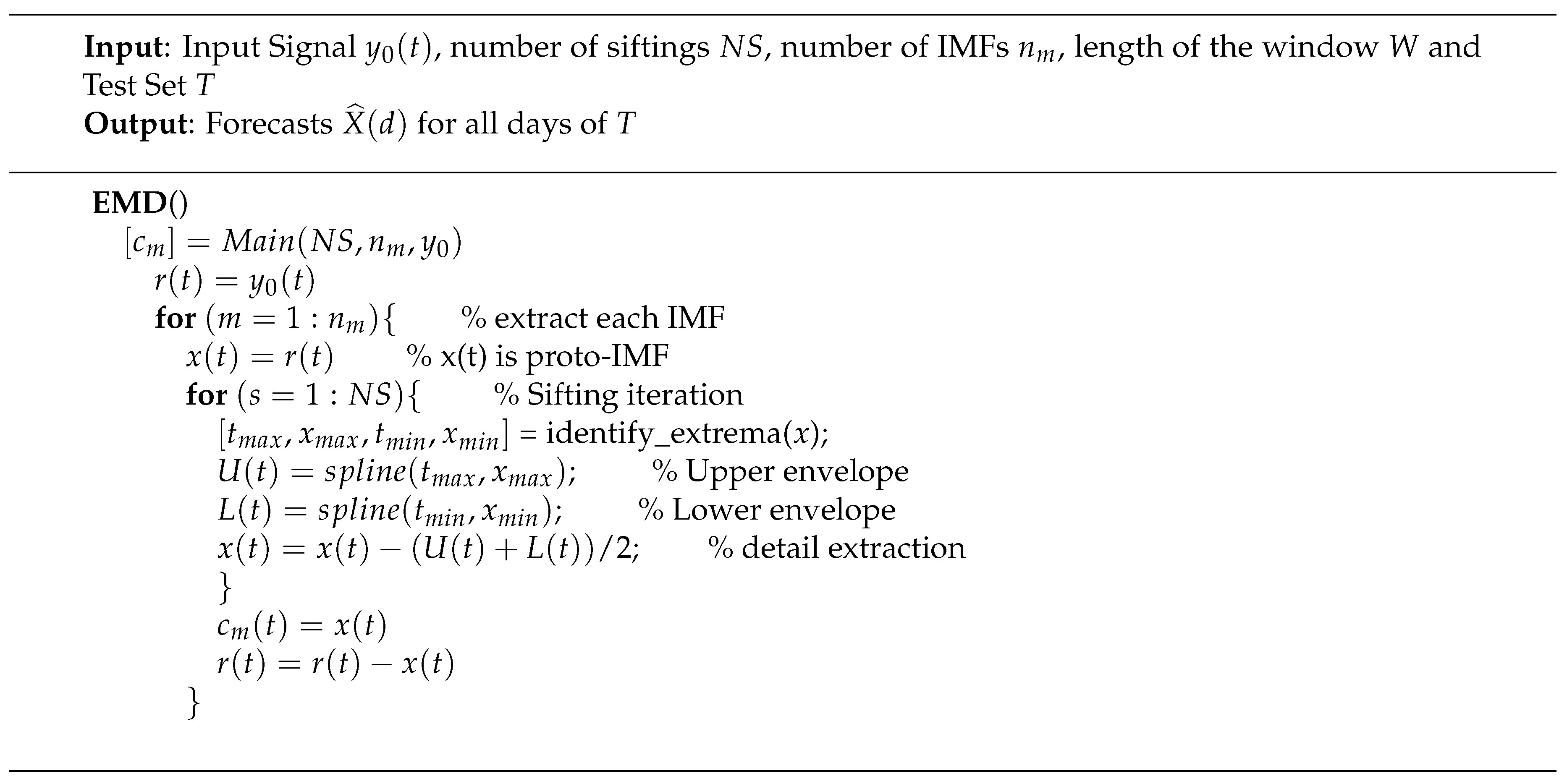
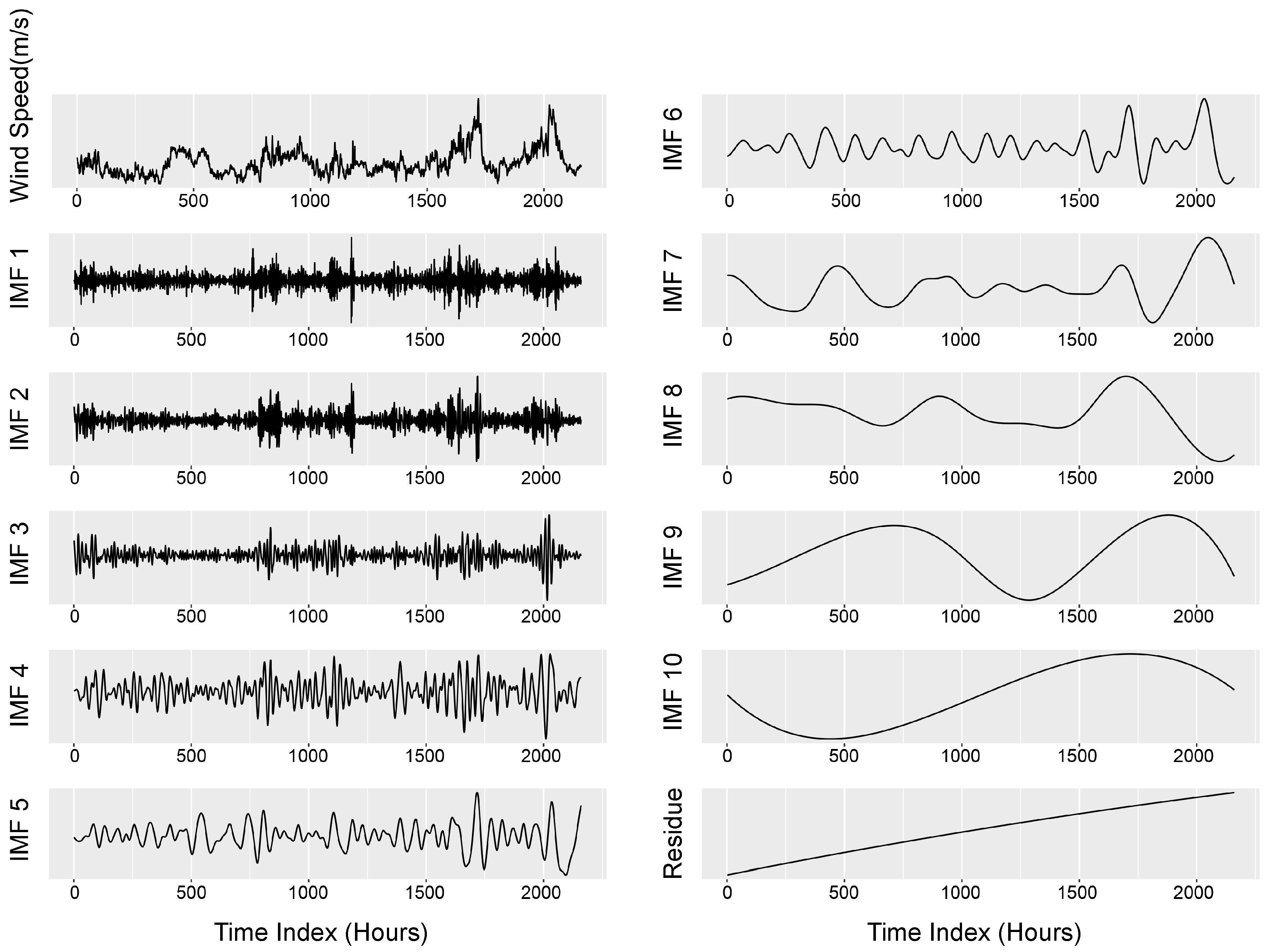
4. Empirical Mode Decomposition

Empirical Mode Decomposition is one of the most commonly used decomposition methods. The concept of EMD is applicable on nonlinear and non-stationary complex time series [85]. The EMD method decomposes such time series into a finite and small number of intrinsic modes along with a residual. These modes are known as IMFs. This decomposition is based only on the time series characteristics itself. Firstly, it identifies all local extrema in the time series and, in corresponding to them, it forms upper and lower envelopes, respectively, with an interpolation method such as a cubic spline. Secondly, the mean of upper and lower envelopes is subtracted from the time series, which leads to generation of a local intrinsic mode function. These two steps are followed until the next conditions are fulfilled:
(1)
the mean of lower and upper envelopes tends to zero, and
(2)
the number of extrema and zero crossing differs at most by one.
This process is called sifting and leads to the generation of finite numbers of IMFs and a residue as shown in Label (1):
x ( t ) = i = 1 N I M F i ( t ) + R N ( t ) ,
where I M F i ( t ) indicates all possible IMFs, N is the number of generated IMFs and R N ( t ) is a residue generated as a result of decomposition.
Figure 5 shows the general scheme for the EMD method and a finite number of IMFs generated with a sample of wind speed data are shown in Figure 6. However, EMD consists of various processes such as IMF extraction, sifting iterations, identification of extrema, generation of upper and lower envelopes and details extraction; the complexity of EMD is equivalent to that of traditional Fourier transform with a larger factor. Both time and space complexities for the EMD method were found to be O ( n . l o g n ) as discussed in [91]. Hence, EMD came out to be a computationally efficient method with simple and effective results with similar complexity as that of contemporary decomposition methods.

5. Improvements in EMD

In EMD, the minima and the maxima of a signal are detected recursively and then the lower, as well as upper envelopes, are detected with interpolation. While generating the envelopes, a low pass filter is used to remove the average of envelopes and high-frequency components retained as a part of IMFs. Hence, minima/maxima detection, interpolation for generation of envelopes and stopping criteria play an important role in the performance of EMD. However, due to the lack of mathematical theories, there is large scope to improve the process of decomposition.
As time elapsed, various modifications were proposed to improve the overall frequency mode segregation and ultimately to remove the mode mixing problem and predict with higher precisions. First of all, the more robust version of EMD was proposed in [92,93]. It used robust optimization techniques for extraction of extrema and formation of envelopes with an interpolation process. Quite different approaches were proposed in [94,95]. In these methods, a variational and recursive decomposition approach to EMD was used. Both of these methods’ robustness was proved in comparison to traditional EMD. In addition, Blakely [96] proposed a superior method which was able to interpolate to a near natural cubic spline fit without solving any equations. This method used a least squares approximation which was free from any matrix calculation and hence eventually it reduced the efforts for complex calculations and a Fast Empirical Mode Decomposition process was achieved.
Another decomposition method apparently inspired by EMD was the Empirical Wavelet Transform (EWT) [97]. EWT explicitly built adaptive wavelets which aided in decomposition of the signal into adaptive bands. Furthermore, Huang and Kunoth [98] proposed an adaptive iterative method to minimize the smoothness function which removes the inequalities in all extrema in each iteration steps. In this way, smooth extrema envelopes were achieved successfully with the proposed optimization method. Similarly, a novel Sliding Window Empirical Mode Decomposition (SWEMD) approach was proposed in [99] which was more suitable for long signals having very high sampling frequency. With this simple improvement in the EMD, a significant rise in computational speed was gained.
Moreover, Wu and Huang [86] proposed the Ensemble Empirical Mode Decomposition (EEMD) method. So far, it is believed to be one of the most esteemed and successful modifications in the conventional EMD method. The motivation behind EEMD was to solve the problem of mode mixing in EMD method. The EEMD is a repetitive method and, in each repetition, EMD is used to decompose the signal data along with a finite Gaussian white noise. For each repetition, Gaussian white noise of different amplitudes was introduced to the signal data. However, for each repetition, the resultant decomposed IMFs were noisier, but finally while calculating the mean of the subseries (IMFs) in all repetitions, the finite white noise canceled each other and more meaningful IMFs were generated.
Furthermore, a minute modification of EEMD was proposed in [100], named Complementary ensemble empirical mode decomposition (CEEMD). The CEEMD used a collection of independent Gaussian white noise and its corresponding complementary pairs instead of fully independent Gaussian white noise as generated in EEMD. Eventually, due to this modification, all white noise parameters canceled each other and made the noise-free reconstruction of original time series and maintained all other advantages of EEMD. Since EEMD and CEEMD were repetitive methods, these suffered the problem of longer computational delays. Torres et al. [101] attempted to solve this problem by introducing an extra noise coefficient vector ‘w’ in order to control the noise level at each decomposition stage and reduced the number of repetitions as compared to EEMD and CEEMD methods.
Later, a quite successful improvement in EMD was proposed in [102]. The authors proposed a model which optimized the decomposition process using an alternative direction method of multipliers approach and named Variation Mode Decomposition (VMD). Since this method had been shown to be theoretically soundproof with ease in understanding, it holds an eminence to overcome the performance of conventional EMD method in various applications.
A recent article [103] proposed a weighted EMD based prediction model which incorporated a feed-forward neural network into the EMD based framework. This approach used the weighted recombination strategy for step ahead prediction. This method improved the meaningful prediction horizon up to a significant level.

6. Motivations for Proceeding with EMD

Conventionally, while implementing any prediction model for wind prediction, the wind data was used directly without its preprocessing. However, due to highly chaotic, intermittent and intrinsic nature of such data, the prediction performance of various models became highly inaccurate, since it became very difficult to understand the patterns or moving tendency of the wind data. However, the wind dataset is sensitive to climate change, temperature, terrain, pressure and the nested yearly, monthly, weekly and daily cycles of the wind [13,39]. Hence, the wind data had combinations of series with different frequencies and possesses nonlinear, fluctuating nature. For the sake of improving the prediction accuracy, the segregation of these series with different frequencies from chaotic wind data was considered to be possible solutions.
With the advances in statistical and machine learning based data analysis methods, there are large numbers of decomposition methods which can be used in segregating the wind data into subseries of different frequencies. Huang et al. [85] claimed that the EMD method has been verified to be more suitable and practical than other little-wave decomposition analysis in many areas. To support this statement for wind prediction applications, this section reviewed the research thoughts, principles and motivations of various researchers for using the EMD method in decomposing the wind data. Though the ultimate goal of all researchers behind the use of EMD was to enhance the forecast precision, many of them have discussed how EMD will be able to achieve it more accurately, efficiently and readily.
Generally, the decomposition based hybrid prediction models are based on the ‘divide and conquer’ strategy for nonlinear and nonstationary data and show better performance than the conventional single models. Such hybrid models used distinct decomposition methods such as Wavelet transform, morphology filters, EMD and many others. The Wavelet transform is not adaptive and adhere to prior knowledge of its mother wavelets and hence somewhat restricts its capability to extract nonlinear and nonstationary components in the data [22,58]. Similarly, the morphology filters have to select the shape and the length of the structural element which has no unified standard and which depends on human experience [104], whereas the EMD method has the great attention of researchers because of its superior performance (even for highly nonlinear and noisy signals) and its easy to understand approach. The following are the impulses for using EMD for decomposition of wind data reported in various articles:
  • In comparison to other decomposition methods, EMD generates relatively stationary subseries (IMFs) which can be easily modeled [35,40,56].
  • All IMFs developed with EMD eliminate stochastic volatility and hence improve the prediction results [7,56].
  • EMD eliminates the noisy patterns, randomness, instability and large fluctuations in the data [12,15,19].
  • Apart from unique signal decomposition, IMFs (generated with EMD) have good local characteristics in both time as well as frequency domains [27].
  • The working principle of EMD is empirical without any mathematical/statistical calculations and hence is very easy to understand [28].
  • EMD is fully data driven and a self-adaptive method [22,56,58].
  • EMD is empirical, intuitive, direct and analyzes multi-component signals with predetermined basis functions [13].
  • EMD can handle complex valued time series very efficiently [54].
  • EMD has good multi-resolution and wide range of applicabilities [33,34].
  • EMD decreases the instability of wind data and hence minimizes the difficulties in high precision predictions [48].
  • Practically, there is no need of data provided at regularly spaced time interval in EMD as by means of the Fourier and Wavelet transform [50,98].
  • Forecasting with EMD is independent of subjective experience, since prior knowledge of data is not required such as wavelet base (as needed in Wavelet transform) [24,26].
  • After addition of all IMFs, the coupling of characteristics information gets reduced and hence original signal gets reconstructed more accurately [26].
These points promoted the EMD over Wavelet transform and other decomposition methods. However, the mode mixing is the problem in EMD which heavily influenced the prediction accuracy in wind applications [33,41,56]. Because of this, sometimes it might be possible that EMD could not decompose the data properly and generate the IMF signals with irregular patterns containing combinations of distinct frequencies. In order to eliminate this problem, the EEMD method was introduced in [86]. The EEMD held all the superior qualities of EMD and along with this, it could effectively extract the features and physical meanings in data set through decomposing the dataset according to the difference of frequencies. Hence, in recent years, most of the researchers have shown their inclination towards EEMD and further modified versions of EMD (such as [100,101]) as compared to the conventional EMD. Additionally, the popularity of EMD methods can be seen with the availability of its packages in different statistical and general purpose languages/tools as shown in Table 3.

7. Intrinsic Mode Functions

In the EMD method, as an outcome of sifting process, finite numbers of IMFs and a residue are generated. Generally, IMF is defined as an amplitude modulated frequency modulated (AM-FM) signal as expressed in Label (2):
V k ( t ) = A k ( t ) c o s ( θ k ( t ) ) ,
where θ k ( t ) (phase component) is a nondecreasing function such that θ k ( t ) > = 0 ; A k ( t ) (envelope component) is nonnegative and θ k ( t ) is much faster than envelope ( A k ( t ) ) and the instantaneous frequency ( θ k ( t ) ). In other words, θ k ( t ) and A k ( t ) are sinusoidal waves and the frequency of θ k ( t ) is higher than the frequency of A k ( t ) .
Usually, in EMD/EEMD based hybrid prediction models, all IMFs and the residue are forecasted individually with time series prediction methods and the corresponding summation of these predicted values are considered to be the final prediction outcomes. The conventional procedure for hybrid EMD/EEMD method is shown in Figure 7. However, with further investigation and further advancement in the time series analysis techniques, the time series of distinct IMFs were categorised in various characteristics. In Refs. [10,19,27,46] and [60], the IMFs were categorized into two bands with high and low frequency components. These articles stated the IMFs with lower frequency bands represent the central tendency of the data and highly regular pattern which shows the accurate characteristics of the original data, whereas the IMFs with higher frequencies contain large quantity of noisy signals, which mainly reflects the random information that led to a great disturbance for prediction precision of wind data.
Refs. [10,19,21,46] confirmed the very weak correlation between the data and the IMFs with higher frequencies and possessing noisy patterns. In most of the cases, the PACF plots were used to decide the correlation between the data and IMFs. Eventually, they claimed that getting rid of high frequency IMFs led to improvement in the forecasting precision in wind applications. Refs. [10,19] removed the first IMF (IMF 1) from the analysis, whereas the first two IMFs were omitted directly in [46]. In contrary to this, Ref. [58] omitted the residue series from the prediction analysis and concluded the prediction results were not much affected with absence of it. However, Refs. [27,37,60] believed that there is potential and useful information involved in IMF 1 and handled this situation differently. Instead of removing high frequency IMFs, both high and low frequency IMFs were predicted with different and more suitable prediction models. In [27], the high frequency IMFs were predicted using a moving average method and the low frequency IMFs with the conventional Persistence approach. Similarly, in [60], the high frequency IMFs were again decomposed and reconstructed by Wavelet transformation. Finally, different LSSVM models were used for each IMF to get final wind speed forecast. Then, for the first time, the highest frequency band (IMF 1) is processed by Singular Spectrum Analysis (SSA) in [37]. SSA is a nonparametric spectral estimation method, which helps in the decomposition of time series into a sum of components, each having a meaningful interpretation. Ultimately, the processed IMF1 and all other components were modeled by Elman Neural Network to get the final wind speed prediction results. Similarly, in [21], low and high frequency components were predicted with the AR model with Kalman filter and LSSVM, respectively.
Nevertheless, the models based on categorized into high and low frequencies of IMFs were able to achieve better prediction accuracy, few other models [24,33,34,58] reported further investigation in the characteristics of different IMFs and the residue. They categorized them into three classes. Xingjie et al. [24] named these classes as high, middle and low frequencies, whereas the same classes were named micro, meso and macro scale subsequences in [58]. However, ultimately, these classes were categorized on the same principle. The high frequency components show highly random information in original wind data and the middle frequency components reflect the periodic and useful signals for prediction. Finally, the very low frequency components show the time series with linear trends in most of the cases. With the consideration of different variation tendencies (high/middle/low frequencies), various models were proposed in [24,33,34]. In [24], the categorization of IMFs into three classes was done through the t-test [107]. Then, the high frequency components were forecasted with Elmar neural network model and middle frequency components with the ARMA model. The remained low frequency IMFs (including the residue) were forecasted with a simple AR model. However, Refs. [24,33,34] claimed that the prediction results of hybrid models such as Genetic Algorithm (GA)—BP neural network or model based on Extreme Learning Machine (ELM) and Least Square Support Vector Machine (LSSVM) have exhibited better prediction results irrespective of nature of frequency components present in each IMF.
Apart from this, another approach is proposed in [22], in which the IMFs generated with EMD were arranged into a matrix. Then, the eigenvalues ( λ ) of that matrix were calculated using SVD method and categorized the IMFs into a trend and stochastic components. On the basis of a specific threshold of eigenvalues, high-frequency IMFs were added to form the stochastic component. Then, the trend component was obtained by subtracting the stochastic component from the original signal. Finally, the trend component was predicted by polynomial regression and the forecast for the stochastic component was carried out by the least-square support vector machine (LSSVM) model.
A quite different and novel approach to optimize the number of IMFs was discussed in [7]. As discussed in Label (1), the conventional EMD method generates a N number of IMFs. The proposed model reduced the number of IMFs nearly to half of original number N in order to reduce the computational complexity. This reduction is achieved by transforming (1) into the new decomposition expression as shown in Label (3):
x ( t ) = i = 1 N ¯ I M F i ( t ) + R N ¯ ( t ) ,
where N ¯ was derived with (round ( N / 2 ) + 1 ) and ‘round’ refers to round-off. Along with this, the residual function was evaluated with expression shown in Label (4).
R N ¯ ( t ) = i = N ¯ + 1 N I M F i ( t ) + R N ( t ) .
In this way, the number of IMFs was significantly reduced from N to N ¯ . This model had claimed that the newly generated IMFs are more volatile and hence increased the accuracy of the prediction model. By observing the performance of various models as discussed in this section, it can be suggested that the better prediction can be achieved if the model is one such as AR, MA, ARMA or ARIMA, built for IMFs with low frequencies and the higher frequency IMFs will be predicted with nonlinear forecasting techniques such as SVM, ANN, Kalman filter, etc.

8. Review on EMD/EEMD Based Ensemble Methods for Wind Data Prediction

As explained in Section 1 and Section 3, the decomposition based prediction methods are broadly classified into three categories, that are artificially intelligent, statistical and chaotic methods. In this work, such methods hybridized with EMD/EEMD methods are reviewed and compared with their simple (without decomposition) forms, which allow us to understand the improvement in the prediction accuracy. This section is devoted to explaining the performance of these hybrid methods in detail. The initial two subsections discuss ANN and SVM methods, followed by various statistical and chaotic methods.

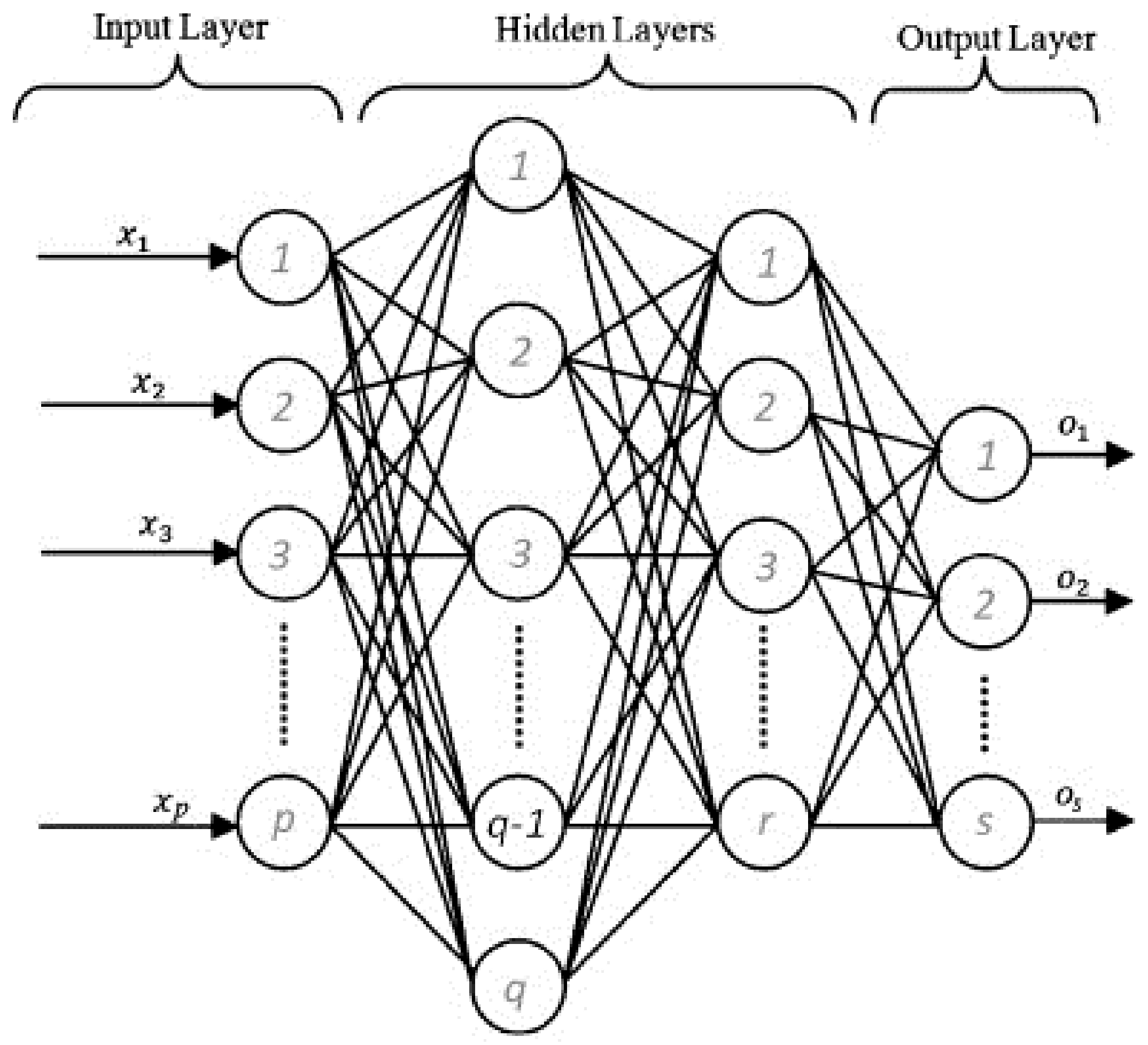
8.1. Artificial Neural Networks

Among artificial intelligence approaches, ANN is one of the most intensively used methods. Generally, it is used in optimization, prediction, pattern classifications, function approximation, regression, automatic control and many others [108]. Normally, a multilayer neural network possesses three or four layers, named an input layer, one or more hidden layers, and an output layer. All these layers are connected to their adjacent layers through some common points known as ‘nodes’. All of these nodes are interconnected through a processing unit called as ‘neurons’. These neurons add their weighted inputs to generate as internal activity level u i given in Label (5):
u i = j = 1 n w i j x i j w i o ,
where w i j and x i j are the weight of connection and input signal number from input j to neuron I, respectively; w i o is the threshold bias of i. The structure of ANN is illustrated in Figure 8 (adopted from [109]). There are a number of training algorithms used in building ANN such as Genetic Algorithm, incremental and batch back propagation, quick propagation, Broydene Fletcher Goldforbe Shanno Quasi network back propagation and many others [47]. However, in the case of wind data predictions, Back Propagation (BP), Elman Neural Network (ENN), Genetic Algorithm Back Propagation (GABP), Radial Basis Function Neural Network (RBFNN), Fuzzy Neural Network (FNN), Wavelet Neural network (WNN) and Levenberg–Marquardt (LM) are the often used training algorithms [12].
BPNN is the most popular neural network, which is a kind of multilayer feed-forward neural network. It uses the gradient descent method to minimize the error between predicted and original values. Back propagation consists of two subprocesses: updating and learning as shown in Labels (6) and (7), respectively:
k i j ( t ) = w i j ( t 1 ) Δ w i j ( t ) ,
Δ w i j ( t ) = η E / w i j ( t 1 ) + α Δ w i j ( t 1 ) ,
where w i j is weight between nodes i and j, t is the current iterative step, n is the learning speed, α is the impulse parameter and E is the error super curve face.
Furthermore, Ref. [110] proposed a GABP neural network, in which the Genetic algorithm is combined with BPNN and optimized the weight and bias values of the BP network while training. The GA optimizes the parameters by applying selection and crossover techniques which are inspired by nature. After BPNN, ENN is another widely used method in wind data predictions. ENN is a well known recurrent network, consisting of four layers: the input layer, the context layer, the hidden layer, and the output layer [36]. Usually, ENN is based on the principle of keeping the equal numbers of hidden and context units. The state equations of ENN are shown in Labels (8) and (9):
x ( t + 1 ) = f ( w i n · p ( t + 1 ) + w · x ( t ) ) ,
y ( t + 1 ) = f o u t ( w o u t · p ( t + 1 ) + r ) ,
where x, p, and t are input, interval and output values and w i n , w, w o u t are the respective weights, f o u t and and r are the output and the internal neurons activation, respectively.
Apart from this, RBFNN is another feed-forward network [111]. However, it contains three layers similar to BPNN and classical neural networks, but there is no weight between hidden layers. In addition, each hidden unit uses the radial activated function. The function obtained at output layers of RBFNN can be written as in Label (10):
y j = i = 1 L ϕ i w i + θ j ,
where w i j is the weight between nodes i and j, L is the number of hidden nodes and θ j is a biased weight of j t h output.
FNN is a further network system whose architecture is based on the combination of a neural network with fuzzy logic. Usually, FNN consists of five layers: the input layer, conditional element layer, rules layer, action element layer and the output layer. The conditional layer uses fuzzification and decides the weights in the network. These weights are provided to rule layer. This rule layer represents a fuzzy rule. Then, the output of rule layer is given to an action element layer which works similarly to a hidden layer in conventional BPNN.
Similarly, WNN is another network which has been used in wind prediction with significant success. Similar to conventional neural networks, WNN consists of three layers: the input, output and hidden layers. In contradiction to classical neural networks, the hidden layer of WNN contains hidden units which are referred as wavelons [112]. These wavelons are similar to neurons used in conventional neural networks and transforms the input variables into diluted versions of mother wavelets and finally provide it to the output layer.
With respect to the training precisions, the LM method based neural network is one of the attractive methods for the feed forward neural network [113]. Because of its accuracy in training precision, this method is widely used in wind prediction applications.
Furthermore, the MLP is another standard feed-forward artificial neural network [114]. The MLP has been generally used in the data analysis and signal processing because of its excellent nonlinear matching and generalization abilities. The standard modeling process of the MLP network can be found in [115].
Additionally, the modification of the traditional single-hidden layer feed-forward based a novel and fast learning algorithm was proposed in [116], named the ELM. The ELM is preferred over traditional neural networks because it randomly assigns the thresholds and weights between the input and hidden layers. In addition, it does not require to adjust these parameters while the learning process. Hence, it can complete the training process extremely fast. Apart from quick learning speed, ELM has better accuracy performance than other ANNs [117].
The RELM is another modification in ELM. The difference between RELM and ELM is that the RELM inherits the simple parameter selection and fast training speed of ELM during adjusting the penalty factor in order to prevent over-fitting problems.
This section is dedicated to the comparison of various neural network models with the hybridization of EMD or EEMD methods for wind speed and power predictions. This comparison is performed on the basis of types of neural networks discussed earlier in this subsection.

8.1.1. EMD-BPNN Models

For short-term wind speed prediction, a standard hybridization of EMD with the BPNN method was proposed in [8], where all IMFs and the residue were forecasted with BPNN models. Similarly, Guo et al. [10] followed the same approach except for the first IMF (IMF1) from the prediction analysis. This study showed that the IMF1 containing high-frequency components is most unsymmetrical and disordered, which leads to the generation of large disturbance in forecasting. In addition, it claimed the performance of this modified model was better than the simple hybrid EMD-BPNN model. Another hybrid EMD-BPNN model was trained with the AdaBoost method [118] was proposed in [9]. In this model, the base learning algorithm with BPNN, trained with AdaBoost on each IMF and the residue.
Later on, Hong et al. [7] proposed a novel EMD-ANN model for both short-term wind speed and power prediction. This model used the correlation coefficient while deciding the useful IMFs among all IMFs generated with the EMD method. In this method, the number of IMFs were reduced to nearly half of the actually generated IMF numbers. The methodology used for selection of numbers of useful IMFs is explained in detail at the end of Section 7. The simulation showed that the proposed model outperformed the conventional neural networks and other state-of-the-art methods. Table 4 shows the percentage improvement in the EMD-BPNN model than simple BPNN models.

8.1.2. EEMD-BPNN Model

Ren et al. [11] proposed a comparative study of EMD and modified versions (EEMD, CEEMD, and CEEMDAN) based prediction models for short-term wind speed predictions. The hybridization of these decomposition methods was performed with BPNN and SVM methods. This article stated that the hybrid model with BPNN method performed better than the simple BPNN model, but the achieved improvement was marginal as compared to that of hybrid SVM models. The percentage improvement in EEMD-BPNN model is discussed in Table 5.

8.1.3. EMD-GABP Model

Wang et al. [32] have discussed the challenges while applying EMD based forecasting models for wind speed data. This article proposed two revised EMD-GABP methods (named Algorithm 1 and Algorithm 2). In both methods, the IMFs generated with EMD were forecasted with GABP methods. The principal difference between these methods was that, in Algorithm 1, the inputs of all steps were determined before the beginning of forecasting, whereas in Algorithm 2, inputs for specific steps were achieved by re-decomposing the time series with newly generated data. This article concluded the inferior results of the EMD based hybrid method. It stated that the EMD based hybrid models have not shown the advantage over the conventional (with decomposition) prediction methods. In addition, the time consumption by such hybrid models was much longer than that of conventional methods.

8.1.4. EEMD-GABP Model

A standard hybrid EEMD-GABP model was proposed in [33,34]. These models have decomposed the wind speed data into IMFs with EEMD and all of these IMFs were forecasted with GABP method. Both of these articles have concluded the superior performance of EEMD based models over that of EMD based models. Table 5 shows the percentage improvement in EEMD-GABP model as compared to simple GABP and EMD-GABP models.

8.1.5. EMD-ENN Model

The standard hybridization of EMD and the ENN was proposed in [35], where all IMFs generated with EMD were forecasted with ENN, whereas, in [24], hybridization of EMD, ENN, ARMA, and AR was used to forecast wind speed data. In this model, the IMFs were differentiated into high, medium and low-frequency components and ENN method was found to be more appropriate for prediction of high-frequency IMFs containing random patterns as compared to ARMA and AR. Both of these models outperformed the single ENN model. Furthermore, Ref. [24] claimed the use of multiple prediction methods in accordance with frequency patterns. The efficiency of such models get enhanced and the forecasting precision further gets improved. The percentage improvement in prediction accuracy with EMD-ENN is shown in Table 6.

8.1.6. EEMD-ENN Model

A novel approach of Secondary Decomposition Algorithm (SDA) was proposed for short-term wind speed prediction in [36]. This proposed algorithm (SDA) combined the Wavelet Packet Decomposition (WPD) and FEEMD. First of all, SDA decomposed the wind speed data into the appropriate components and the detailed components. Furthermore, the detailed component was decomposed into finite numbers of IMFs with FEEMD. This proposed model (WPD-FEEMD-ENN) showed the satisfactory prediction results and improved the performance of hybrid WPD-ENN and simple ENN models significantly. In addition, this model outperformed various hybrid models with distinct decomposition methods.
Furthermore, Ref. [37] proposed three hybrid models using ENN, EMD and its advanced versions (EEMD and CEEMDN) improved by SSA [119] for short-term wind speed prediction. The high-frequency IMFs obtained with EMD, EEMD, and CEEMDN methods were further handled with the SSA method. Ultimately, through the retreatment of SSA, the proposed hybrid models significantly improved the prediction accuracy. As compared to single ENN, EMD-ENN, and other models, all three proposed models showed more accurate forecasting results as discussed in Table 7.

8.1.7. EMD-RBFNN Model

Zheng et al. [38] proposed a hybrid EMD-RBFNN model for short-term wind power prediction. The model showed a standard approach, in which all IMFs generated with EMD were forecasted with the RBFNN method. The proposed method demonstrated high prediction precision and adaptability as compared to traditional ANN models as shown in Table 8.

8.1.8. EEMD-FNN Model

Short-term wind speed prediction with the FNN method using EEMD and Cuckoo Search (CS) methods [120] was proposed in [44]. In this hybrid model, EEMD was employed to remove the high-frequency noise associated with wind speed series and CS was used to optimize the parameters of FNN model. This study showed that the proposed hybrid model outperformed simple FNN and other models with more accuracy for wind speed datasets.

8.1.9. EEMD-WNN Model

Another EEMD and neural network based hybrid method which used the CS optimization method was proposed in [46]. This model was based on hybridization of the WNN and EEMD methods. In addition, the CS method was used to optimize the parameters of WNN model. Moreover, the first two IMFs (containing high frequencies and noise components) were removed directly from the prediction analysis. This model improved the multi-step forecasting performance and appeared to be more suitable for implementing in wind farms.

8.1.10. EMD-LMNN Model

A standard approach of hybridization of EMD and LMNN was proposed in [47]. All IMFs generated by EMD were forecasted with suitable LMNN models, whereas a novel approach of a combination of decomposition method (EMD) and the prediction methods (LMNN and SVM) was proposed in [14]. In contrast to the standard approach (used in [47]), Zhang et al. [14] discussed the Decomposition Selection Forecasting (DSF) approach. In DSF, after generating IMFs, the initial input–output pairs were constructed from all IMFs and the original data. Then, they extracted the relevant and informative features using the feature selection process. Ultimately, a suitable predictive model was estimated using these selected features. The disparity between DSF and standard approach was that the DSF did not build the prediction models for all IMFs as it had been done in the standard approach. The performance of the proposed model was satisfactory for short-term wind speed prediction as compared to traditional EMD based hybrid and single neural network models.

8.1.11. EEMD-MLP Models

Liu et al. [49] compared four hybrid models with the MLP method. These models used four different decomposition methods: WD, WPD, EMD and FEEMD. This comparative study concluded that the FEEMD-MLP model showed the best performance in three step predictions and WPD-MLP in one step predictions. In addition, all hybrid models of MLP performed better than those of the ANFIS method, which uses the NN and Fuzzy interface system.
Furthermore, the modified model of [49] was discussed in [48]. Since the superiority of FEEMD was already experienced in [49], models in [48] have applied FEEMD with the MLP method using two optimization methods: Mind Evolutionary Algorithm (MEA) and GA. This study investigated the performance of MLP neural network by the FEEMD method optimized with MEA and GA methods. Finally, the study concluded that the hybrid FEEMD-MEA-MLP model had outperformed all other models under study and respective improvements in accuracy is illustrated in Table 9.

8.1.12. EEMD-ELM Models

Liu et al. [55] compared four hybrid models with hybridization of different decomposition methods and the ELM method. WD, WPD, EMD, and FEEMD were the decomposition methods used in the comparison study. For wind speed data, the FEEMD had shown best performance for three step forecasting and WPD showed better results for one and two step forecasting. In addition, as compared to WD and EMD, the WPD and FEEMD showed better prediction accuracy in all step predictions.
Similarly, Ref. [56] examined the performance of RELM with WD, EMD, and FEEMD decomposition methods. In this study, for short-term wind prediction, the FEEMD-RELM model performed best among all methods under study and poorest performance was shown by the hybrid WD-RELM method among all hybrid methods. Table 10 shows the percentage of improvements in EEMD-ELM model as compared to a simple ELM model.

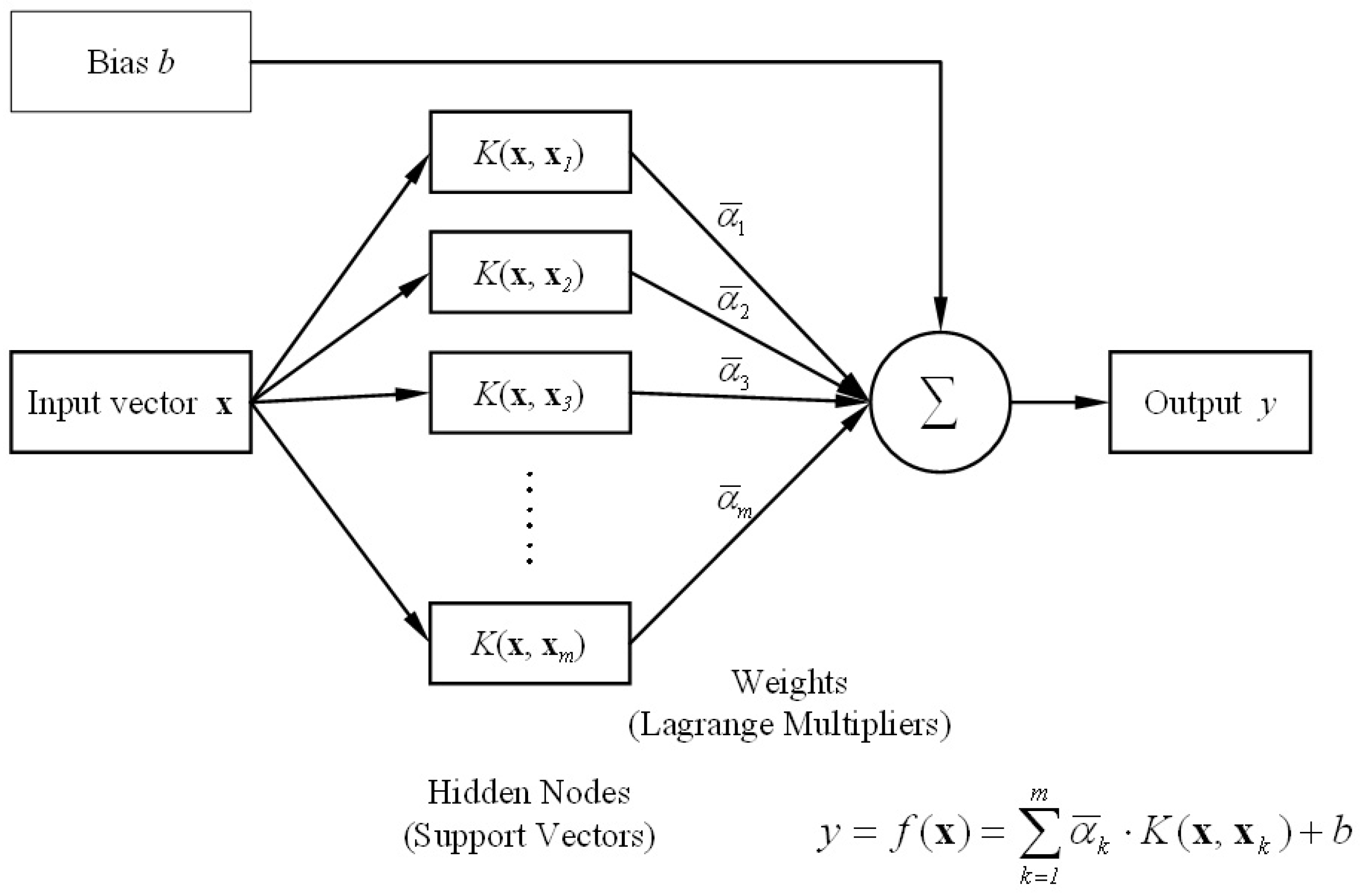
8.2. Support Vector Machines and Least Square SVM

The SVM [121] is an elegant method based on statistical learning principles for nonlinear classification, function estimation, and pattern recognition applications. It possesses a feed-forward network design with a nonlinear hidden layer. SVMs follow the concept of decision planes that define the decision boundaries and these decision planes are nothing but the boundary between a set of objects from different classes. Figure 9 (adopted from [122]) shows the architecture of an SVM method. The concept behind the SVM or regression is the mapping of a dataset into a high dimensional feature space through a nonlinear mapping. After mapping, the SVM performs a linear regression in that feature space.
LSSVM method is another advanced formulation of SVM regression proposed in [123] which defines a cost function different from simple SVM and reduces the complex calculations significantly related to quadratic equations. This eventually accelerates the solution speed notably. The detailed comparison of SVM and LSSVM is discussed in [124].
This section is focused on the comparison of EMD and EEMD based hybrid SVM and LSSVM models for wind speed and wind power prediction applications. In this paper, 19 related papers have been reviewed; most of these hybrid models were used EMD as decomposition method, whereas, in recent years, researchers proposed models aided with the superiority of EEMD methods and achieved the better prediction results. The performance of each hybrid models is discussed in this section with both SVM and LSSVM methods.
All articles reviewed in this section were predicting future values for next few hours or a day and hence it can be generalized that the EMD/EEMD-SVM/LSSVM models were used for short-term wind speed and power data. This section is further divided into five subsections with distinct combinations as EMD-SVM, EEMD-SVM, EMD-LSSVM, EEMD-LSSVM and other modified models.

8.2.1. EMD-SVM Models

In Refs. [16,17,18], the simplest combinations of hybrid EMD-SVM models were used. As usual, these models decomposed the wind data into a series of components (IMFs) using EMD and then different models were built with different kernel functions and parameters for each component with the SVM model. Both Refs. [17,18] used the EMD-SVM model on wind speed data, while [18] further converted the predicted speed data into wind power data through a practical wind power curve, whereas Ref. [16] operated the EMD-SVM model directly on the wind power data. The hybrid EMD-SVR model with input vector lagged by 1 is proposed in [13]. In this novel model [13], a vector containing one historical data is combined with each IMF and the residue generated with EMD to train the SVR for all IMFs.
In addition to this, the attempt to improve prediction accuracy is made with the use of an improved Cuckoo Search parameter estimation algorithm with the hybrid EMD-SVR model in [15]. In this model, the parameters in SVM models were optimized by SDCS model which is a combination of the CS algorithm and the Steepest Descent (SD) method.
Zhang et al. [14] proposed an EMD-SVM model with the aid of a feature selection technique. Initially, the wind speed data is decomposed into a finite number of IMFs by EMD and then the input variables (initial features) and targets were constructed from all IMFs and the original data. Finally, a feature selection technique is used to derive the relevant and useful features and future values were predicted by SVM using these selected features. Authors named this hybrid model the Decomposition Selection Forecasting (DSF) model. Unlike conventional models, in the DSF model, predictive models were not built for each IMF.
All hybrid EMD-SVM models discussed in this subsection have outperformed the simple SVM model with RMSE and MAE as performance measures as shown in Table 11.

8.2.2. EEMD-SVM Models

It is said that the problem of mode mixing in EMD was the motivation behind the birth of EEMD method. Large numbers of articles in distinct research areas have claimed the superior performance of EEMD method over hybrid EMD models. For wind speed data, Refs. [11,19,20] used hybrid EEMD-SVM model and achieved better prediction accuracy than other state-of-the-art models. In [20], wind speed data was decomposed into seven IMF components with EEMD and then all IMFs were predicted with appropriate SVM models. A similar approach was used in [19], where the high-frequency IMF (IMF1) was removed from the prediction analysis and all remaining IMFs were forecasted with suitable SVM models.
Furthermore, the EEMD-SVM model along with two modified EEMD methods were proposed in [11]. This article compared the prediction performance of EEMD-SVM, CEEMD-SVM and CEEMDAN-SVM models with the conventional simple SVM and EMD-SVM models. In addition, equivalent models with hybrid ANN methods (EEMD-ANN, CEEMD-ANN, and CEEMDAN-ANN) were examined in the study. The result showed that the hybrid model of SVM with EEMD and its improved versions had enhanced the prediction significantly as compared to other methods including hybrid ANN models. The CEEMDAN-SVM model was observed to be the best model. The percentage of improvement in error parameters (RMSE, MAE, and MAPE) with EEMD-SVM model relative to SVM and EMD-SVM models were reported in Table 12.

8.2.3. EMD-LSSVM Models

In 2002, LSSVM [123] come out to be a more successful modification in the conventional SVM method. This subsection reviews the hybrid EMD-LSSVM model used for wind speed and power predictions. The very first articles proposing EMD-LSSVM model for wind data [39,59] are the only articles which applied LSSVM for prediction of all IMFs generated with EMD method. Furthermore, the models proposed for such applications were comprised of hybridization of more than two methods. Such as [60], they used two decomposition methods (EMD and WT) along with the LSSVM method. First of all, the time series was decomposed in multiple subseries and the subseries with higher frequencies were further decomposed with WT. Finally, the LSSVM method that forecasted all subseries and wind speed prediction was performed.
Whereas Refs. [21,22,58] examined the time series characteristics of IMSs and tested its effects on prediction, Refs. [21,22] differentiated the IMFs into high and low-frequency components and operated these distinct frequency components with different prediction methods. In [21], high-frequency IMFs were predicted with the LSSVM and remaining low frequencies were predicted with AR model with Kalman filter. Similarly, in [22], the high frequency and stochastic components were predicted with LSSVM methods and the remaining trend components were forecasted with polynomial regression. The aggregation of values predicted with both models derived the final wind speed prediction and then converted into wind power data with a historical data based power curve. Liang et al. [58] claimed that the residue component is either a constant or a monotonic function and hence prediction accuracy will be independent from it. This model omitted the residue from the analysis and predicted wind power with a hybrid EMD-LSSVM, ELM model.
All the hybrid EMD-LSSVM models have concluded their better prediction accuracy and minimum error as compared to the simple LSSVM model and other contemporary methods. Table 13 shows the improvement in prediction with EMD-LSSVM as compared to the LSSVM method.

8.2.4. EEMD-LSSVM Models

For wind speed/power data, hybrid models based on EEMD and LSSVM had been proposed very recently. Interestingly, most of the authors showed the research outcomes in directly predicting wind power data with the hybrid EEMD-LSSVM model instead of predicting wind speed and then converting it into wind power. Since these are recent articles, the authors seem convinced with earlier research articles discussing the importance of hybridization of more number of methods in a model to predict more accurately by using the positive behavior of all methods. In [41], hybridization of four methods (EEMD, PCA, LSSVM, and BA) was used to predict one step ahead wind power. Initially, the wind power data was decomposed into IMFs and then PCA was used to reduce the number of modeling inputs with the identification of significant variables which are maintaining most of the information belonging to the data. Finally, the LSSVM model accompanying the BA was developed to predict the subseries (IMFs). The intention of adoption of BA was to ensure the generalization and the learning ability of LSSVM. Safari et al. [42] showed a novel chaotic time series analysis model for wind power prediction. As usual, EEMD decomposed the wind power data into finite numbers of IMF and then the chaotic time series analysis is applied to discover the chaotic components present in these IMFs. Then, the SSA was applied to the chaotic IMFs and, finally, LSSVM was used to predict one step ahead values. In addition, the several steps ahead prediction with greater accuracy was made possible with the multi-scale SSA (MSSSA) by maintaining general trends of chaotic components and making them smoother with the elimination of extremely rapid change with low amplitudes.
A quite similar and a bit complex approach was used in recent article [40] for wind speed prediction. In this model, after decomposition with EEMD, kernel density estimation based Kullback–Leibler divergence and energy measures (feature selection methods) were adopted to reduce the disturbance of chaotic components. Ultimately, the LSSVM method is applied to establish one step ahead prediction. Apart from this, the hybrid of LSSVM and the generalized autoregressive conditionally heteroscedastic model was proposed to correct the error component, whenever their inherent correlation and heteroscedasticity could not be neglected. All articles [40,41,42] claimed the superior performance of EEMD-LSSVM model with few improvements over simple LSSVM and EMD-LSSVM as shown in Table 14.
However, in 2015, another modification in EEMD was used for wind speed prediction in [43]. This model used FEEMD method for decomposition and Bat algorithm to optimize the parameter selection for LSSVM models for all IMFs. Sun et al. [43] concluded that the proposed (FEEMS-BA-LSSVM) model outperformed the similar models with decomposition methods such as EMD, WT with a combination of optimization methods including BA, HS, and PSO.

8.2.5. EMD-RVM Models

An EMD based hybrid model with a combination of Relevance Vector Machine (RVM) was studied in [50] for short-term wind power predictions. RVM is a popular regression and classification method which is defined as a sparse Bayesian extension version of SVM. In the proposed model, with standard prediction flow, all IMFs generated with EMD were predicted with RVM models and achieved a good prediction performance for wind power data.
Furthermore, Ref. [51] proposed a hybrid model of EMD and Multi-Kernel Relevance Vector Regression Algorithm (EMD-MkRVR) for short-term wind speed prediction. MkRVR is based on RVM with the use of RBF and polynomial kernel. The properties of polynomial kernel were determined by controlled parameters and then its performance was compared with RBF kernel RVR (RBFRVR) and the polynomial kernel RVR (PolyRVR) models. At the end, the superior performance of the MkRVR algorithm was concluded for short-term wind speed predictions.

8.2.6. EEMD-RVM Models

Another short-term wind speed forecasting model was introduced in [52] which hybridized the EEMD and RVM methods optimized by the Cloud Adaptive Particle Swarm Optimization (CAPSO) algorithm. In this method, the RVM models were used according to the characteristics of each IMF, and the aggregation of each component forecasting results produces the final forecasting values. The novelty of this model was the selection of a kernel function of RVM. This method used the typical Gaussian kernel function optimized with the CAPSO algorithm. Eventually, it showed the great influence on the RVM model forecasting performance. The hybrid EEMD-RVM model showed superior forecasting results and led to reduction of the wind speed prediction error.
Further, Ref. [53] proposed a short-term wind power interval forecasting model based on EEMD, RVM and Runs Test (RT). This model used the RT method to reconstruct the EEMD generated IMF components and obtained three new components (Trend, Detailed and Random) characterized by the fine-to-coarse order. Finally, the RVM is applied on trend components to achieve point forecasts as well as on both detailed and random components to achieve interval forecasts. The overall prediction was obtained with a combination of prediction outcomes of all components. Table 15 shows the percentage of improvement in models proposed in [52,53] as compared to the simple RVM models.

8.3. Statistical Models

Autoregression method based models are one of the most often used prediction models. These models are based on the regression of a time series with its previous values. Likewise, in a simplest autoregression model, a value from a time series is regressed on its previous values as shown in Label (11).
y t = β 0 + β 1 y t 1 + ϵ t .
where y t is an original time series at time interval t; β 0 and β 1 are the constants; and ϵ t is an error associated with the linear regression process.
In such a model, the response variable in the time period of one acts as the predictor. Depending on the time lag of the predictor, the order of an autoregression has been decided and hence the preceding model is a first-order autoregression AR(1). Furthermore, with integration of a few other methods such as MA methods, these simple Autoregression models get advanced in various forms such as ARMA, ARIMA methods and many others. Out of these, the ARIMA method has successfully outperformed many prediction models in distinct applications.
The ARIMA method is the combination of differencing, autoregression and the moving average model [125]. To design an ARIMA model for time series data, it is mandatory to check whether the data is stationary. If the time series data is not stationary, the differencing technique is used to make it stationary. If a time series contains upward or downward trends, then the first order differencing can be applied. In addition, if the time series is a curve pattern, then logarithmic treatments may be applied with the differencing, whereas if the time series data shows some repeated pattern after a specific interval of time, the seasonal differencing can be the solution to make that data stationary. Applying differencing techniques is nothing but the computation of differences between consecutive observations, whereas seasonal differences are the difference between actual observations and their corresponding special time lagged observations.
The autocorrelation function is the popular method to examine the non-stationarity of time series and can be converted into stationary series with the differencing method. Once the time series data becomes stationary, ARIMA uses an autoregression method to forecast the variable with possible combinations of past values of that variable. Along with this, the ARIMA model applies the moving average method. This method uses past prediction errors obtained in other methods like regression to assist in forecasting the variable more accurately. The combination of autoregression, differences, and moving average methods in ARIMA model is given as A R I M A ( p , d , q ) , where d is the degree of differencing, p and q are the order of autoregressions and moving average method, respectively. The linear expression to state the ARIMA method is shown in Label (12).
( 1 B ) d Y t = μ + θ ( B ) ϕ ( B ) α t ,
where t is the indexed time, μ is the mean term, B is the backshift operator such that B Y t = T t 1 . Furthermore, θ ( B ) and ϕ ( B ) are the autoregressive and the moving-average operator, respectively, and α t is the error term at time t.

8.3.1. EMD-Autoregression Models

This section describes the performance of various hybrid EMD/EEMD models in association with distinct ARIMA family methods. As usual, these models were initiated with the decomposition of wind data into more stationary and regular components (IMFs and residue) using the EMD/EEMD method. With the decomposition, the interruption and coupling between all IMF components get reduced and chances of more accurate prediction get enhanced.
While comparing the various hybrid EMD models with autoregression family methods, EMD-ARMA were found to be very common models for wind data prediction. For the first time, hybridization of EMD and ARMA was proposed in [26] in which all IMF and residue wind speed data generated with EMD were unconditionally predicted with suitable ARMA models. Similarly, Liu et al. [25] used the same prediction methodology on wind speed data and finally transformed the prediction results in terms of wind power.
Furthermore, Xingjie et al. [24] proposed a model with conditional use of the ARMA method along with autoregression and ANN methods. With this model, the IMF with higher and lower frequency components were predicted with ANN and AR methods, respectively, whereas, the ARMA method was used in predicting the IMF containing middle frequency components and the final wind speed prediction performance was examined for direct multi-step and iterative multi-step approaches. In a similar way, Ref. [27] proposed a model, in which higher frequency IMFs were forecasted using the Moving Average method and the low frequency IMFs were predicted with the traditional Persistence approach.
The hybridization of EMD with the combination of LSSVM and autoregression methods were proposed for wind speed in [21] and wind power in [22], respectively. In both models, the IMFs (and residue) with very low-frequency components were forecasted with the autoregression method and remaining higher frequency IMFs were predicted with the LSSVM method.
Ren et al. [11] proposed the EMD-RARIMA model, which used a modified ARIMA method, named Recursive ARIMA (RARIMA) method. In this model, all IMFs and the residue were forecasted with suitable RARIMA models and this hybrid model outperformed the state-of-the-art methods such as BPNN, simple ARIMA, and persistent random walk method. Table 16 shows the percentage of improvement in EMD-ARMA model as compared to simple ARMA models.

8.3.2. EEMD-Autoregression Model

For wind datasets, the only model which has used EEMD with an autoregression method is observed in [28]. This model proposed a hybrid model combining EEMD, ANFIS and SARIMA methods for short-term wind speed prediction. ANFIS is a model which integrates the impact of neural networks and fuzzy interface system. The further combination with SARIMA method led to more accurate and effective prediction results. In this model, the nonlinear IMFs were predicted with ANFIS models and SARIMA was applied to periodic IMF series as shown in Table 17.
By comparing the performance of all models discussed in this subsection, the following points were observed:
  • The hybridization of EMD/EEMD with an autoregression model improved the prediction accuracy as compared to simple autoregression models for wind data sets.
  • In most of the models (reviewed in this section), the autoregression methods were combined with other methods such as ANN and LSSVM and were found to be more suitable for low-frequency components, while the other methods were kept restricted for IMFs with higher frequency components.

8.3.3. EMD-kNN Model

The k Nearest Neighbor (kNN) method is a lazy learning process [126], used for both classification and regression. The kNN is a non-parametric statistical model and applied in a wide range of applications. Ref. [54] proposed two configurations of a hybrid EMD-kNN model, in which EMD was followed by a kNN for short-term wind speed forecasting. The two configurations of EMD-kNN were EMD-kNN-P and EMD-kNN-M. In the EMD-kNN-P model, kNN was applied on each decomposed IMF and the residue for separate modelling and forecasting followed by aggregation. While EMD-kNN-M formed a feature vector set from all IMFs and residue followed by a single kNN modelling and forecasting. For short-term wind speed forecasting, EMD-kNN-M showed better prediction accuracy than simple kNN and EMD-kNN-P models for various datasets. Table 18 shows the percentage of improvement in EMD-kNN-M model for one of the datasets used in [54].

8.3.4. EEMD-PSF Model

Furthermore, another promising statistical univariate time series forecasting method named Pattern Sequence based Forecasting (PSF) was proposed over the last decade, by Martínez-Álvarez et al. [127]. The prediction performance of PSF method depends on pattern sequences present in a time series data. It is a combination of distinct processes such as data normalization, clustering, averaging, forecasting and denormalization. The PSF method uses labels for different patterns existing in time series data, instead of the original time series data. The detailed methodology of PSF method is discussed in [70,127]. Ref. [45] proposed a hybrid EEMD-PSF model, in which EEMD was followed by a PSF for 12 and 24 h step ahead wind speed forecasting. In the proposed model, PSF was applied on each decomposed IMF and the residue for separate modelling and forecasting followed by aggregation. The selection of optimum window size and cluster size for the corresponding IMF is discussed in the source article. Table 19 shows the percentage of improvement in EEMD-PSF model for the Galician datasets used in [45].

8.4. Chaotic Theory Treatments

Usually, a strongly nonlinear, complex and nonstationary nature of wind power data shows highly chaotic characteristics. Refs. [29,30,31] proposed hybrid models based on chaotic theory principles to minimize the effects of chaotic nature of measured data on the prediction accuracy.
In [30], all IMFs generated with EMD were examined for their chaotic characteristics. Those IMFs found to be chaotic were predicted with the Largest Lyapunov Exponent Prediction method [128], while the remaining IMFs including the residue were predicted with the Grey forecasting method [129]. The chaotic nature of IMFs was examined with the Wolf method [128], which is used to calculate the Largest Lyapunov exponent. The prediction results showed a good prediction accuracy with the proposed method for short-term wind power data.
However, in [29,31], the Local First Order (LFO) [130] and Echo State network (ESN) [131] methods were used, respectively. The motivation behind using these methods was to handle the chaotic wind power IMFs generated with EMD. Both of these articles concluded better prediction accuracy as compared to respective simple (without EMD) models.

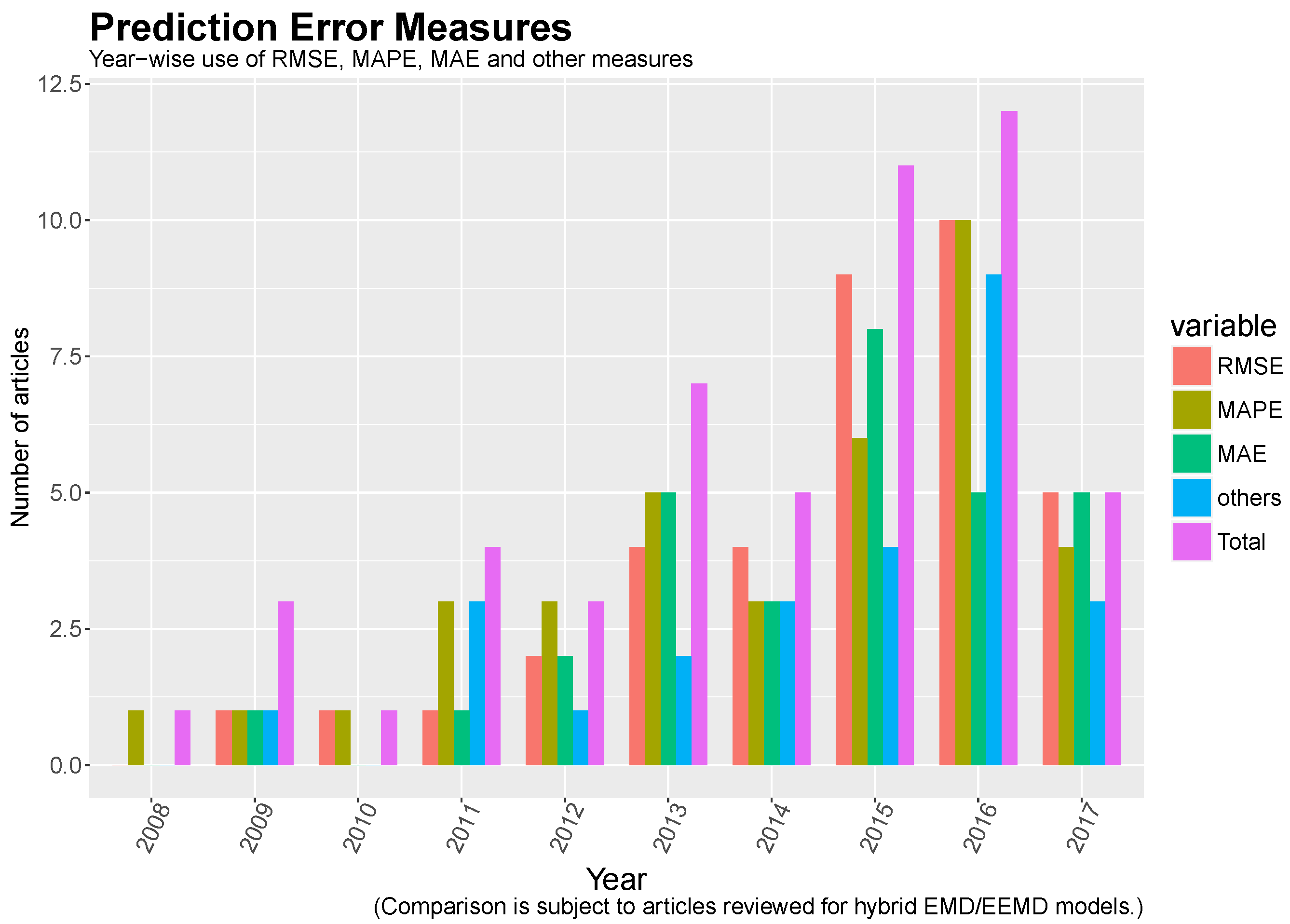
9. Measures to Estimate Prediction Errors

The performance of any prediction model is usually judged with the goodness by observing its prediction errors. The accurate and meaningful estimation of the prediction error is always of critical importance in prediction applications. A large number of statistical methodologies have been developed for such considerations. Specifically, in wind power and wind speed data prediction applications, the short-term prediction approach is more favorable and known because of its usability. In almost all papers discussed in this review article, with consideration of data from several months and then with the direct or iterated prediction approach, prediction performance is measured for next few hours or few days. In research case studies, this prediction performance is evaluated by comparing the predicted outcomes with the actually measured datasets. Usually, this comparison is performed with various statistical methods, known as prediction error measures.
Table 20 shows the combinations of prediction error measures (RMSE, MAPE and MAE) used in articles using hybrid EMD/EEMD models for wind data. From this table, it is observed that RMSE, MAPE, and MAE are widely accepted error measures for short-term wind prediction. These measures evaluate the statistical errors between actual and predicted values cumulatively. However, in earlier days, sample-wise comparison of relative forecasting error was very common. Han and Zhu [17] and Xingjie et al. [24] showed the relative errors for all the samples present in the forecasting samples. As the time elapsed, RMSE, MAPE and MAE measures became more popular and came out to be very much useful and informative. So far, the MAPE and RMSE are the most commonly used measures for performance of prediction models. RMSE simply averages the squares of the differences between actual and predicted values and then calculates the square root of the averaged value. The RMSE describes the sample standard deviation of a predicted value from the corresponding measured values.
Similarly, MAPE describes the accurate sensitivity for a small change in data and hence it is more useful when larger errors are more acceptable for larger measured values [132]. The MAPE is an average of the absolute errors in terms of percentages of the measured values, whereas MAE is similar to RMSE, in which, instead of squaring, MAE uses absolute values and averages the differences. MAE describes the average variance between measured and predicted values. These RMSE, MAE and MAPE are defined as shown in Labels (13), (14) and (15), respectively:
R M S E = 1 N i = 1 N X i X ^ i 2 ,
M A E = 1 N i = 1 N X i X ^ i ,
M A P E = 1 N i = 1 N X i X ^ i X i × 100 % ,
where X i is the measured data and X ^ i is predicted data at time t. N is the data size for the prediction process.
Figure 10 shows the year-wise use of RMSE, MAE and MAPE measures in wind speed or power prediction with hybrid EMD/EEMD methods, whereas overall use of these measures is illustrated in Figure 11. It can be observed that most of the articles have used RMSE and MAPE as prediction error comparison measures, whereas MAE was found to be another widely used measure for wind prediction. Along with these standard measures, many researchers have used some other measures such as Absolute Errors (AE), Mean Square Error (MSE), Mean Absolute Scaled Error (MASE), coefficient of determination ( R 2 ), Absolute Percentage Error (APE), Mean Squared Prediction Error (MSPE), Mean Relative Error (MRE), Square Sum Error (SSE), Mean Relative Percentage Error (MRPE), Root Mean Square Relative Error (RMSRE), Forecasting Interval Coverage Percentage (FICP), Forecasting Interval Average Width (FIAW) and Standard Deviation (SD). In addition, some articles have adopted a few statistical tests instead of error measures to evaluate the performance of prediction models which include Wilcoxon Signed Rank Test (WSRT) and Friedman Test. Similarly, there can be a variety of various error measures and a statistical test for understanding the error accuracy of a particular model. However, still, RMSE, MAPE, and MAE seem to be more suitable for wind speed and power prediction applications because of its simplicity and meaningful statistical significances. Since these measures are used in the majority of the research articles, these achieve a status of state-of-the-art error performance measures and ease in the comparison with the earlier proposed model’s results.

10. Discussion

Three questions can be asked after having classified all the papers mentioned throughout this review.
The first one asks the researchers about the usefulness of the analyzed methods. Furthermore, a very interesting question to answer is if all these methods can be applied in industry or if they simply have interest from an academic point of view. With regard to this, and according to the authors’ observations, it can be said that researchers have also been using similar and even more complex methods in a variety of applications. For instance, for studying noise reduction in several types of turbines, for weather forecasting and some other purposes. In this sense, it must be said that applications such as the ones studied are actually needed, and, in many cases, are easy to understand and their use is simple, and not only from an academic point of view, but also for industry. In general, patterns present in time series can be easily extracted, and this helps researchers and developers predict with more accuracy. In most of the cases, EMD methods are used for this purpose.
A second question in this discussion is about the possible obsolescence of some of the methods under scrutiny. It has been observed that researchers tend to avoid the basic EMD model and this must be said. However, modified versions of it such as EEMD and FEEMD are still very popular among scientists and, as has been shown along the paper, they have been of common use in many recent papers.
Another interesting question is related to hardware and software developments. Machine learning and other concepts that have been developed over the last few decades make researchers reflect about the possibilities of future developments, i.e., the future of methods such as those studied in the paper. In this respect, it can be anticipated that future developments and modifications of the EMD method will offer many possibilities of improvement in results obtained in the simulations where these methods are used.

11. Conclusions

This paper presents a wide review of empirical decomposition methods applied to wind speed and wind power prediction. It is being assumed that wind speed and wind power prediction techniques can be classified into three different groups, known as the physical, the statistical and the intelligent approaches. However, the fact should not be forgotten that many researchers have claimed hybrid methods to constitute a fourth approach.
The paper focuses on the comparison between the existing methods reviewed and the new methods obtained by hybridizing those methods with empirical model decomposition processes and their modified versions as pre-processing techniques. The main conclusion of this work is that the comparison seems to be always in favor of the hybridized methods, which prove their superiority with respect to the non-hybridized ones.
It must be noticed that case studies differ very much among different papers. The authors have used multiple datasets, locations, step sizes, conditions, seasons or dates. Hence, the difficulty of including all those comparison results is actually great. This is the reason why in this work only results of a few cases from each reviewed paper are presented. The main goal here is to make the researchers see the evidence of the improvement of hybridization.
Apart from this, it becomes very difficult to quantify the overall improvement in prediction accuracy with the hybridization of the EMD method, but this paper confirms the popularity and penetration of hybrid neural network and support vector machine based models in wind speed and power predictions. In addition, the innovations in treatment for distinct IMFs as discussed in Section 7 have enlarged the scope for further improvements in performance of hybrid models.
There is a big contingent of known techniques and this involves also important difficulties for establishing clear comparisons among them, except for the above commented fact that hybridized methods gave better results in all simulated cases. A comparison of all studied methods depends on so many different nuances that the best way of extracting some conclusions is by reading the presented tables with attention.

Author Contributions

Conceptualization, N.B. and A.F.; Methodology, N.B. and A.F.; Software, N.B.; Validation, N.B., A.F. and D.V.; Formal Analysis, D.V.; Investigation, A.F.; Resources, N.B., K.K. and A.F.; Data curation, N.B. and A.F.; Writing—Original Draft Preparation, A.F., K.K. and N.D.; Writing—Review and Editing, D.V and K.K.; Visualization, N.B.; Supervision, A.F. and D.V.; Project Administration, A.F. and K.K.

Funding

This research received no external funding.

Acknowledgments

Neeraj Bokde was supported by the R&D project work undertaken under the Visvesvaraya PhD Scheme of the Ministry of Electronics and Information Technology, Government of India, being implemented by Digital India Corporation (Bengaluru, India).

Conflicts of Interest

The authors declare no conflict of interest.

Abbreviations

The following abbreviations are used in this manuscript:
ANFISAdaptive Neural Network based Fuzzy Interface System
ANNArtificial Neural Networks
ARAutoregression
ARIMAAutoregressive Integrated Moving Average
ARMAAutoregressive Moving Average
BABat Algorithm
BPNNBack-Propagation Neural Networks
CEEMDComplete Ensemble Empirical Mode Decomposition
CEEMDANComplete Ensemble Empirical Mode Decomposition with Adaptive Noise
CSCuckoo Search
DSFDecomposition Selection Forecasting
ELMExtreme Learning Machine
EEMDEnsemble Empirical Mode Decomposition
EMDEmpirical Mode Decomposition
ENNElman Neural Networks
ESNEcho State Network
EWTEmpirical Wavelet Transform
FEEMDFast Ensemble Empirical Mode Decomposition
FNNFeed-forward Neural Network
GABPGenetic Algorithm Back-Propagation Neural Network
HSHarmony Search
IMFIntrinsic Mode Function
kNNk - Nearest Neighbors
LFOLocal First Order
LMNNLevenberg-Marquardt Neural Network
LSSVMLeast Squares Support Vector Machine
MAMoving Average
MAEMean Absolute Error
MAPEMean Absolute Percentage Error
MEAMind Evolutionary Algorithm
MkRVRMultiple-kernel Relevance Vector Regression
MLPMultilayer Perceptron
MMLPMathematical Morphologybased Local Predictor
MTDMean Trend Detector
NWPNumerical Weather Prediction
PACFPartial Auto-correlation Function
PCAPrinciple Component Analysis
PolyRVRPolynomial kernel Multiple-kernel Relevance Vector Regression
PSFPattern Sequence based Forecasting
PSOParticle Swarm Optimization
RARIMARecursive Autoregression of Integrated Moving Average
RBFNNRadial Basis Function Network
RELMRegularized Extreme Learning Machine
RMSERoot Mean Square Error
RTRuns Test
RVMRelevance Vector Machine
SARIMASeasonal Autoregressive Integrated Moving Average
SDStandard Deviation
SSASingular Spectrum Analysis
SVDSingular Value Decomposition
SVMLeast Squares Support Vector Machine
SWEMDSliding Window Empirical Mode Decomposition
VMDVariation Mode Decomposition
WDWavelet Decomposition
WNNWeighted Neural Network
WPDWavelet Packet Decomposition
WTWavelet Transform

References

  1. Yuan, X.; Chen, C.; Yuan, Y.; Huang, Y.; Tan, Q. Short-term wind power prediction based on LSSVM–GSA model. Energy Convers. Manag. 2015, 101, 393–401. [Google Scholar] [CrossRef]
  2. Zhu, X.; Genton, M.G. Short-Term Wind Speed Forecasting for Power System Operations. Int. Stat. Rev. 2012, 80, 2–23. [Google Scholar] [CrossRef] [Green Version]
  3. Erdem, E.; Shi, J. ARMA based approaches for forecasting the tuple of wind speed and direction. Appl. Energy 2011, 88, 1405–1414. [Google Scholar] [CrossRef]
  4. Lydia, M.; Kumar, S.S.; Selvakumar, A.I.; Kumar, G.E.P. A comprehensive review on wind turbine power curve modeling techniques. Renew. Sustain. Energy Rev. 2014, 30, 452–460. [Google Scholar] [CrossRef]
  5. Carrillo, C.; Montaño, A.O.; Cidrás, J.; Díaz-Dorado, E. Review of power curve modelling for wind turbines. Renew. Sustain. Energy Rev. 2013, 21, 572–581. [Google Scholar] [CrossRef]
  6. Shi, J.; Qu, X.; Zeng, S. Short-term wind power generation forecasting: Direct versus indirect arima-based approaches. Int. J. Green Energy 2011, 8, 100–112. [Google Scholar] [CrossRef]
  7. Hong, Y.Y.; Yu, T.H.; Liu, C.Y. Hour-ahead wind speed and power forecasting using empirical mode decomposition. Energies 2013, 6, 6137–6152. [Google Scholar] [CrossRef]
  8. Liu, H.; Chen, C.; Tian, H.Q.; Li, Y.F. A hybrid model for wind speed prediction using empirical mode decomposition and artificial neural networks. Renew. Energy 2012, 48, 545–556. [Google Scholar] [CrossRef]
  9. Ren, Y.; Qiu, X.; Suganthan, P.N. Empirical mode decomposition based adaboost-backpropagation neural network method for wind speed forecasting. In Proceedings of the 2014 IEEE Symposium on Computational Intelligence in Ensemble Learning, Orlando, FL, USA, 9–12 December 2014; pp. 1–6. [Google Scholar]
  10. Guo, Z.; Zhao, W.; Lu, H.; Wang, J. Multi-step forecasting for wind speed using a modified EMD-based artificial neural network model. Renew. Energy 2012, 37, 241–249. [Google Scholar] [CrossRef]
  11. Ren, Y.; Suganthan, P.; Srikanth, N. A comparative study of empirical mode decomposition-based short-term wind speed forecasting methods. IEEE Trans. Sustain. Energy 2015, 6, 236–244. [Google Scholar] [CrossRef]
  12. Zhang, W.; Qu, Z.; Zhang, K.; Mao, W.; Ma, Y.; Fan, X. A combined model based on CEEMDAN and modified flower pollination algorithm for wind speed forecasting. Energy Convers. Manag. 2017, 136, 439–451. [Google Scholar] [CrossRef]
  13. Ren, Y.; Suganthan, P.N.; Srikanth, N. A novel empirical mode decomposition with support vector regression for wind speed forecasting. IEEE Trans. Neural Netw. Learn. Syst. 2016, 27, 1793–1798. [Google Scholar] [CrossRef] [PubMed]
  14. Zhang, C.; Wei, H.; Zhao, J.; Liu, T.; Zhu, T.; Zhang, K. Short-term wind speed forecasting using empirical mode decomposition and feature selection. Renew. Energy 2016, 96, 727–737. [Google Scholar] [CrossRef]
  15. Wang, C.; Wu, J.; Wang, J.; Hu, Z. Short-Term Wind Speed Forecasting Using the Data Processing Approach and the Support Vector Machine Model Optimized by the Improved Cuckoo Search Parameter Estimation Algorithm. Math. Probl. Eng. 2016, 2016, 4896854. [Google Scholar] [CrossRef]
  16. Zhang, W.; Liu, F.; Zheng, X.; Li, Y. A hybrid EMD-SVM based short-term wind power forecasting model. In Proceedings of the 2015 IEEE PES Asia-Pacific Power and Energy Engineering Conference (APPEEC), Brisbane, QLD, Australia, 15–18 November 2015; pp. 1–5. [Google Scholar]
  17. Han, Z.H.; Zhu, X.X. Training set of support vector regression extracted by empirical mode decomposition. In Proceedings of the 2011 IEEE Asia-Pacific Power and Energy Engineering Conference (APPEEC), Wuhan, China, 25–28 March 2011; pp. 1–4. [Google Scholar]
  18. Lin, Y.; Peng, L. Combined model based on EMD-SVM for short-term wind power prediction. Proc. Chin. Soc. Electr. Eng. 2011, 31, 102–108. [Google Scholar]
  19. Hu, J.; Wang, J.; Zeng, G. A hybrid forecasting approach applied to wind speed time series. Renew. Energy 2013, 60, 185–194. [Google Scholar] [CrossRef]
  20. Jia, S. A new method for the short-term wind speed forecasting. In Proceedings of the 4th International Conference on Electric Utility Deregulation and Restructuring and Power Technologies (DRPT), Weihai, China, 6–9 July 2011; pp. 1320–1324. [Google Scholar]
  21. Tatinati, S.; Veluvolu, K.C. A hybrid approach for short-term forecasting of wind speed. Sci. World J. 2013, 2013, 548370. [Google Scholar] [CrossRef] [PubMed]
  22. Hong, D.; Ji, T.; Zhang, L.; Li, M.; Wu, Q. An indirect short-term wind power forecast approach with multi-variable inputs. In Proceedings of the Innovative Smart Grid Technologies-Asia (ISGT-Asia), Melbourne, VIC, Australia, 28 November–1 December 2016; pp. 793–798. [Google Scholar]
  23. Liu, H.; Tian, H.Q.; Li, Y.F. An EMD-recursive ARIMA method to predict wind speed for railway strong wind warning system. J. Wind Eng. Ind. Aerodyn. 2015, 141, 27–38. [Google Scholar] [CrossRef]
  24. Liu, X.; Mi, Z.; Li, P.; Mei, H. Study on the multi-step forecasting for wind speed based on EMD. In Proceedings of the International Conference on Sustainable Power Generation and Supply, Nanjing, China, 6–7 April 2009; pp. 1–5. [Google Scholar]
  25. Liu, X.J.; Mi, Z.Q.; Bai, L.; Wu, T. A novel approach for wind speed forecasting based on EMD and time-series analysis. In Proceedings of the Asia-Pacific Power and Energy Engineering Conference, Wuhan, China, 27–31 March 2009; pp. 1–4. [Google Scholar]
  26. Li, R.; Wang, Y. Short-term wind speed forecasting for wind farm based on empirical mode decomposition. In Proceedings of the International Conference on Electrical Machines and Systems, Wuhan, China, 17–20 October 2008; pp. 2521–2525. [Google Scholar]
  27. Sun, C.; Yuan, Y.; Li, Q. A new method for wind speed forecasting based on empirical mode decomposition and improved persistence approach. In Proceedings of the Conference on Power & Energy (IPEC), Ho Chi Minh City, Vietnam, 12–14 December 2012; pp. 659–664. [Google Scholar]
  28. Zhang, J.; Wei, Y.; Tan, Z.F.; Ke, W.; Tian, W. A hybrid method for short-term wind speed forecasting. Sustainability 2017, 9, 596. [Google Scholar] [CrossRef]
  29. Drisya, G.; Kumar, K.S. Empirical mode decomposition and chaos based prediction model for wind speed oscillations. In Proceedings of the Conference on Recent Advances in Intelligent Computational Systems (RAICS), Trivandrum, India, 10–12 December 2015; pp. 306–311. [Google Scholar]
  30. An, X.; Jiang, D.; Zhao, M.; Liu, C. Short-term prediction of wind power using EMD and chaotic theory. Commun. Nonlinear Sci. Numer. Simul. 2012, 17, 1036–1042. [Google Scholar] [CrossRef]
  31. Zhang, X.Q.; Liang, J. Chaotic time series prediction model of wind power based on ensemble empirical mode decomposition-approximate entropy and reservoir. Acta Phys. Sin. 2013, 62, 50505. [Google Scholar]
  32. Wang, Y.; Wu, L.; Wang, S. Challenges in applying the empirical mode decomposition based hybrid algorithm for forecasting renewable wind/solar in practical cases. In Proceedings of the Power and Energy Society General Meeting (PESGM), Boston, MA, USA, 17–21 July 2016; pp. 1–5. [Google Scholar]
  33. Wang, Y.; Wang, S.; Zhang, N. A novel wind speed forecasting method based on ensemble empirical mode decomposition and GA-BP neural network. In Proceedings of the Power and Energy Society General Meeting (PES), Vancouver, BC, Canada, 21–25 July 2013; pp. 1–5. [Google Scholar]
  34. Wang, S.; Zhang, N.; Wu, L.; Wang, Y. Wind speed forecasting based on the hybrid ensemble empirical mode decomposition and GA-BP neural network method. Renew. Energy 2016, 94, 629–636. [Google Scholar] [CrossRef]
  35. Wang, J.; Zhang, W.; Li, Y.; Wang, J.; Dang, Z. Forecasting wind speed using empirical mode decomposition and Elman neural network. Appl. Soft Comput. 2014, 23, 452–459. [Google Scholar] [CrossRef]
  36. Liu, H.; Tian, H.Q.; Liang, X.F.; Li, Y.F. Wind speed forecasting approach using secondary decomposition algorithm and Elman neural networks. Appl. Energy 2015, 157, 183–194. [Google Scholar] [CrossRef]
  37. Yu, C.; Li, Y.; Zhang, M. Comparative study on three new hybrid models using Elman Neural Network and Empirical Mode Decomposition based technologies improved by Singular Spectrum Analysis for hour-ahead wind speed forecasting. Energy Convers. Manag. 2017, 147, 75–85. [Google Scholar] [CrossRef]
  38. Zheng, Z.W.; Chen, Y.Y.; Zhou, X.W.; Huo, M.M.; Zhao, B.; Guo, M. Short-term wind power forecasting using empirical mode decomposition and RBFNN. Int. J. Smart Grid Clean Energy 2013, 2, 192–199. [Google Scholar] [CrossRef]
  39. Sun, C.; Yuan, Y. Wind Speed Prediction Based on Empirical Mode Decomposition and Improved LS-SVM. In Proceedings of the 2nd IET Renewable Power Generation Conference (RPG 2013), Beijing, China, 9–11 September 2013. [Google Scholar]
  40. Jiang, Y.; Huang, G. Short-term wind speed prediction: Hybrid of ensemble empirical mode decomposition, feature selection and error correction. Energy Convers. Manag. 2017, 144, 340–350. [Google Scholar] [CrossRef]
  41. Wu, Q.; Peng, C. Wind power generation forecasting using least squares support vector machine combined with ensemble empirical mode decomposition, principal component analysis and a bat algorithm. Energies 2016, 9, 261. [Google Scholar] [CrossRef]
  42. Safari, N.; Chung, C.; Price, G. A Novel Multi-Step Short-Term Wind Power Prediction Framework Based on Chaotic Time Series Analysis and Singular Spectrum Analysis. IEEE Trans. Power Syst. 2017, 33, 590–601. [Google Scholar] [CrossRef]
  43. Sun, W.; Liu, M.; Liang, Y. Wind speed forecasting based on FEEMD and LSSVM optimized by the bat algorithm. Energies 2015, 8, 6585–6607. [Google Scholar] [CrossRef]
  44. Wang, J.; Jiang, H.; Han, B.; Zhou, Q. An experimental investigation of FNN model for wind speed forecasting using EEMD and CS. Math. Probl. Eng. 2015, 2015, 464153. [Google Scholar] [CrossRef]
  45. Bokde, N.; Feijóo, A.; Kulat, K. Analysis of differencing and decomposition preprocessing methods for wind speed prediction. Appl. Soft Comput. 2018, 71, 926–938. [Google Scholar] [CrossRef]
  46. Zhang, K.; Qu, Z.; Wang, J.; Zhang, W.; Yang, F. A novel hybrid approach based on cuckoo search optimization algorithm for short-term wind speed forecasting. Environ. Prog. Sustain. Energy 2017, 36, 943–952. [Google Scholar] [CrossRef]
  47. Dokur, E.; Kurban, M.; Ceyhan, S. Hybrid model for short-term wind speed forecasting using empirical mode decomposition and artificial neural network. In Proceedings of the 9th International Conference on Electrical and Electronics Engineering (ELECO), Bursa, Turkey, 26–28 November 2015; pp. 420–423. [Google Scholar]
  48. Liu, H.; Tian, H.; Liang, X.; Li, Y. New wind speed forecasting approaches using fast ensemble empirical model decomposition, genetic algorithm, mind evolutionary algorithm and artificial neural networks. Renew. Energy 2015, 83, 1066–1075. [Google Scholar] [CrossRef]
  49. Liu, H.; Tian, H.Q.; Li, Y.F. Comparison of new hybrid FEEMD-MLP, FEEMD-ANFIS, Wavelet Packet-MLP and Wavelet Packet-ANFIS for wind speed predictions. Energy Convers. Manag. 2015, 89, 1–11. [Google Scholar] [CrossRef]
  50. Bao, Y.; Wang, H.; Wang, B. Short-term wind power prediction using differential EMD and relevance vector machine. Neural Comput. Appl. 2014, 25, 283–289. [Google Scholar] [CrossRef]
  51. Fei, S.W. A hybrid model of EMD and multiple-kernel RVR algorithm for wind speed prediction. Int. J. Electr. Power Energy Syst. 2016, 78, 910–915. [Google Scholar] [CrossRef]
  52. Zang, H.; Liang, Z.; Guo, M.; Qian, Z.; Wei, Z.; Sun, G. Short-term wind speed forecasting based on an EEMD-CAPSO-RVM model. In Proceedings of the PES Asia-Pacific Power and Energy Engineering Conference (APPEEC), Xi’an, China, 25–28 October 2016; pp. 439–443. [Google Scholar]
  53. Zang, H.; Fan, L.; Guo, M.; Wei, Z.; Sun, G.; Zhang, L. Short-Term Wind Power Interval Forecasting Based on an EEMD-RT-RVM Model. Adv. Meteorol. 2016, 2016, 8760780. [Google Scholar] [CrossRef]
  54. Ren, Y.; Suganthan, P. Empirical mode decomposition-k nearest neighbor models for wind speed forecasting. J. Power Energy Eng. 2014, 2, 176–185. [Google Scholar] [CrossRef]
  55. Liu, H.; Tian, H.Q.; Li, Y.F. Four wind speed multi-step forecasting models using extreme learning machines and signal decomposing algorithms. Energy Convers. Manag. 2015, 100, 16–22. [Google Scholar] [CrossRef]
  56. Sun, W.; Liu, M. Wind speed forecasting using FEEMD echo state networks with RELM in Hebei, China. Energy Convers. Manag. 2016, 114, 197–208. [Google Scholar] [CrossRef]
  57. Soman, S.S.; Zareipour, H.; Malik, O.; Mandal, P. A review of wind power and wind speed forecasting methods with different time horizons. In Proceedings of the North American Power Symposium (NAPS), Arlington, TX, USA, 26–28 September 2010; pp. 1–8. [Google Scholar]
  58. Liang, Z.; Liang, J.; Zhang, L.; Wang, C.; Yun, Z.; Zhang, X. Analysis of multi-scale chaotic characteristics of wind power based on Hilbert–Huang transform and Hurst analysis. Appl. Energy 2015, 159, 51–61. [Google Scholar] [CrossRef]
  59. Wang, X.; Hui, L. One-month ahead prediction of wind speed and output power based on EMD and LSSVM. In Proceedings of the International Conference on Energy and Environment Technology, Guilin, China, 16–18 October 2009; Volume 3, pp. 439–442. [Google Scholar]
  60. Dejun, L.; Hui, L.; Zhonghua, M. One hour ahead prediction of wind speed based on data mining. In Proceedings of the 2nd International Conference on Advanced Computer Control (ICACC), Shenyang, China, 27–29 March 2010; Volume 5, pp. 199–203. [Google Scholar]
  61. Zhang, Y.; Wang, J. K-nearest neighbors and a kernel density estimator for GEFCom2014 probabilistic wind power forecasting. Int. J. Forecast. 2016, 32, 1074–1080. [Google Scholar] [CrossRef]
  62. Pinson, P.; Kariniotakis, G. Conditional prediction intervals of wind power generation. IEEE Trans. Power Syst. 2010, 25, 1845–1856. [Google Scholar] [CrossRef]
  63. Alexiadis, M.; Dokopoulos, P.; Sahsamanoglou, H.; Manousaridis, I. Short-term forecasting of wind speed and related electrical power. Sol. Energy 1998, 63, 61–68. [Google Scholar] [CrossRef]
  64. Damousis, I.G.; Alexiadis, M.C.; Theocharis, J.B.; Dokopoulos, P.S. A fuzzy model for wind speed prediction and power generation in wind parks using spatial correlation. IEEE Trans. Energy Convers. 2004, 19, 352–361. [Google Scholar] [CrossRef]
  65. Barbounis, T.; Theocharis, J. A locally recurrent fuzzy neural network with application to the wind speed prediction using spatial correlation. Neurocomputing 2007, 70, 1525–1542. [Google Scholar] [CrossRef]
  66. Al-Yahyai, S.; Charabi, Y.; Al-Badi, A.; Gastli, A. Nested ensemble NWP approach for wind energy assessment. Renew. Energy 2012, 37, 150–160. [Google Scholar] [CrossRef]
  67. Perrone, T.J.; Miller, R.G. Generalized exponential Markov and model output statistics: A comparative verification. Mon. Weather Rev. 1985, 113, 1524–1541. [Google Scholar] [CrossRef]
  68. Guo, Z.; Dong, Y.; Wang, J.; Lu, H. The forecasting procedure for long-term wind speed in the Zhangye area. Math. Probl. Eng. 2010, 2010, 684742. [Google Scholar] [CrossRef]
  69. Liu, H.; Tian, H.Q.; Li, Y.F. Comparison of two new ARIMA-ANN and ARIMA-Kalman hybrid methods for wind speed prediction. Appl. Energy 2012, 98, 415–424. [Google Scholar] [CrossRef]
  70. Bokde, N.; Asencio-Cortés, G.; Martínez-Álvarez, F.; Kulat, K. PSF: Introduction to R Package for Pattern Sequence Based Forecasting Algorithm. R J. 2017, 9, 324–333. [Google Scholar]
  71. Bokde, N.; Troncoso, A.; Asencio-Cortés, G.; Kulat, K.; Martínez-Álvarez, F. Pattern sequence similarity based techniques for wind speed forecasting. In Proceedings of the International Work-Conference on Time Series, Granada, Spain, 18–20 September 2017; Universidad de Granada: Granada, Spain, 2017. in press. [Google Scholar]
  72. Bokde, N.; Wakpanjar, A.; Kulat, K.; Feijóo, A. Robust performance of PSF method over outliers and random patterns in univariate time series forecasting. In Proceedings of the International Technology Congress, Pune, India, 28–29 December 2017. [Google Scholar]
  73. Louka, P.; Galanis, G.; Siebert, N.; Kariniotakis, G.; Katsafados, P.; Pytharoulis, I.; Kallos, G. Improvements in wind speed forecasts for wind power prediction purposes using Kalman filtering. J. Wind Eng. Ind. Aerodyn. 2008, 96, 2348–2362. [Google Scholar] [CrossRef] [Green Version]
  74. Veluvolu, K.; Ang, W. Estimation and filtering of physiological tremor for real-time compensation in surgical robotics applications. Int. J. Med. Robot. Comput. Assist. Surg. 2010, 6, 334–342. [Google Scholar] [CrossRef] [PubMed]
  75. Zhang, W.; Wu, J.; Wang, J.; Zhao, W.; Shen, L. Performance analysis of four modified approaches for wind speed forecasting. Appl. Energy 2012, 99, 324–333. [Google Scholar] [CrossRef]
  76. Bilgili, M.; Sahin, B.; Yasar, A. Application of artificial neural networks for the wind speed prediction of target station using reference stations data. Renew. Energy 2007, 32, 2350–2360. [Google Scholar] [CrossRef]
  77. Mohandes, M.A.; Halawani, T.O.; Rehman, S.; Hussain, A.A. Support vector machines for wind speed prediction. Renew. Energy 2004, 29, 939–947. [Google Scholar] [CrossRef]
  78. Fazelpour, F.; Tarashkar, N.; Rosen, M.A. Short-term wind speed forecasting using artificial neural networks for Tehran, Iran. Int. J. Energy Environ. Eng. 2016, 7, 377–390. [Google Scholar] [CrossRef] [Green Version]
  79. Rodriguez, C.P.; Anders, G.J. Energy price forecasting in the Ontario competitive power system market. IEEE Trans. Power Syst. 2004, 19, 366–374. [Google Scholar] [CrossRef]
  80. Lydia, M.; Kumar, S.S. A comprehensive overview on wind power forecasting. In Proceedings of the International Power Electronics Conference, Singapore, 27–29 October 2010; pp. 268–273. [Google Scholar]
  81. Ren, Y.; Suganthan, P.; Srikanth, N. Ensemble methods for wind and solar power forecasting—A state-of-the-art review. Renew. Sustain. Energy Rev. 2015, 50, 82–91. [Google Scholar] [CrossRef]
  82. Wu, Y.K.; Hong, J.S. A literature review of wind forecasting technology in the world. In Proceedings of the IEEE Lausanne Power Tech, Lausanne, Switzerland, 1–5 July 2007; pp. 504–509. [Google Scholar]
  83. Kani, S.P.; Ardehali, M. Very short-term wind speed prediction: A new artificial neural network–Markov chain model. Energy Convers. Manag. 2011, 52, 738–745. [Google Scholar] [CrossRef]
  84. Wang, J.; Hu, J. A robust combination approach for short-term wind speed forecasting and analysis–Combination of the ARIMA (Autoregressive Integrated Moving Average), ELM (Extreme Learning Machine), SVM (Support Vector Machine) and LSSVM (Least Square SVM) forecasts using a GPR (Gaussian Process Regression) model. Energy 2015, 93, 41–56. [Google Scholar]
  85. Huang, N.E.; Shen, Z.; Long, S.R.; Wu, M.C.; Shih, H.H.; Zheng, Q.; Yen, N.C.; Tung, C.C.; Liu, H.H. The empirical mode decomposition and the Hilbert spectrum for nonlinear and non-stationary time series analysis. Proc. R. Soc. Lond. A Math. Phys. Eng. Sci. 1998, 454, 903–995. [Google Scholar] [CrossRef]
  86. Wu, Z.; Huang, N.E. Ensemble empirical mode decomposition: A noise-assisted data analysis method. Adv. Adapt. Data Anal. 2009, 1, 1–41. [Google Scholar] [CrossRef]
  87. Fei, S.W.; He, Y. Wind speed prediction using the hybrid model of wavelet decomposition and artificial bee colony algorithm-based relevance vector machine. Int. J. Electr. Power Energy Syst. 2015, 73, 625–631. [Google Scholar] [CrossRef]
  88. An, X.; Jiang, D.; Liu, C.; Zhao, M. Wind farm power prediction based on wavelet decomposition and chaotic time series. Expert Syst. Appl. 2011, 38, 11280–11285. [Google Scholar] [CrossRef]
  89. Katsigiannis, Y.; Tsikalakis, A.; Georgilakis, P.; Hatziargyriou, N. Improved wind power forecasting using a combined neuro-fuzzy and artificial neural network model. In Advances in Artificial Intelligence; Springer: Berlin, Germany, 2006; pp. 105–115. [Google Scholar]
  90. Okumus, I.; Dinler, A. Current status of wind energy forecasting and a hybrid method for hourly predictions. Energy Convers. Manag. 2016, 123, 362–371. [Google Scholar] [CrossRef]
  91. Wang, Y.H.; Yeh, C.H.; Young, H.W.V.; Hu, K.; Lo, M.T. On the computational complexity of the empirical mode decomposition algorithm. Phys. A: Stat. Mech. Appl. 2014, 400, 159–167. [Google Scholar] [CrossRef]
  92. Meignen, S.; Perrier, V. A new formulation for empirical mode decomposition based on constrained optimization. IEEE Signal Process. Lett. 2007, 14, 932–935. [Google Scholar] [CrossRef]
  93. Pustelnik, N.; Borgnat, P.; Flandrin, P. A multicomponent proximal algorithm for empirical mode decomposition. In Proceedings of the 20th European Signal Processing Conference (EUSIPCO), Bucharest, Romania, 27–31 August 2012; pp. 1880–1884. [Google Scholar]
  94. Hou, T.Y.; Shi, Z. Adaptive data analysis via sparse time-frequency representation. Adv. Adapt. Data Anal. 2011, 3, 1–28. [Google Scholar] [CrossRef]
  95. Feldman, M. Time-varying vibration decomposition and analysis based on the Hilbert transform. J. Sound Vib. 2006, 295, 518–530. [Google Scholar] [CrossRef]
  96. Blakely, C.D. A Fast Empirical Mode Decomposition Technique for Nonstationary Nonlinear Time Series; Elsevier Science: New York, NY, USA, 2005; Volume 3. [Google Scholar]
  97. Gilles, J. Empirical wavelet transform. IEEE Trans. Signal Process. 2013, 61, 3999–4010. [Google Scholar] [CrossRef]
  98. Huang, B.; Kunoth, A. An optimization based empirical mode decomposition scheme. J. Comput. Appl. Math. 2013, 240, 174–183. [Google Scholar] [CrossRef]
  99. Stepien, P. Sliding window empirical mode decomposition-its performance and quality. EPJ Nonlinear Biomed. Phys. 2014, 2, 14. [Google Scholar] [CrossRef]
  100. Yeh, J.R.; Shieh, J.S.; Huang, N.E. Complementary ensemble empirical mode decomposition: A novel noise enhanced data analysis method. Adv. Adapt. Data Anal. 2010, 2, 135–156. [Google Scholar] [CrossRef]
  101. Torres, M.E.; Colominas, M.A.; Schlotthauer, G.; Flandrin, P. A complete ensemble empirical mode decomposition with adaptive noise. In Proceedings of the International Conference on Acoustics, Speech and Signal Processing (ICASSP), Prague, Czech Republic, 22–27 May 2011; pp. 4144–4147. [Google Scholar]
  102. Dragomiretskiy, K.; Zosso, D. Variational mode decomposition. IEEE Trans. Signal Process. 2014, 62, 531–544. [Google Scholar] [CrossRef]
  103. Jun, W.; Lingyu, T.; Yuyan, L.; Peng, G. A weighted EMD-based prediction model based on TOPSIS and feed forward neural network for noised time series. Knowl. Based Syst. 2017, 132, 167–178. [Google Scholar] [CrossRef]
  104. Matsuoka, F.; Takeuchi, I.; Agata, H.; Kagami, H.; Shiono, H.; Kiyota, Y.; Honda, H.; Kato, R. Morphology-based prediction of osteogenic differentiation potential of human mesenchymal stem cells. PLoS ONE 2013, 8, e55082. [Google Scholar] [CrossRef]
  105. Kim, D.; Oh, H.S. EMD: A package for empirical mode decomposition and Hilbert spectrum. R J. 2009, 1, 40–46. [Google Scholar]
  106. Luukko, P.; Helske, J.; Räsänen, E. Introducing libeemd: A program package for performing the ensemble empirical mode decomposition. Comput. Stat. 2016, 31, 545–557. [Google Scholar] [CrossRef]
  107. Zimmerman, D.W. Teacher’s corner: A note on interpretation of the paired-samples t test. J. Educ. Behav. Stat. 1997, 22, 349–360. [Google Scholar] [CrossRef]
  108. Mohandes, M.A.; Rehman, S.; Halawani, T.O. A neural networks approach for wind speed prediction. Renew. Energy 1998, 13, 345–354. [Google Scholar] [CrossRef]
  109. Wijayasekara, D.; Manic, M.; Sabharwall, P.; Utgikar, V. Optimal artificial neural network architecture selection for performance prediction of compact heat exchanger with the EBaLM-OTR technique. Nucl. Eng. Des. 2011, 241, 2549–2557. [Google Scholar] [CrossRef]
  110. Duan, G.; Yu, Y. Problem-specific genetic algorithm for power transmission system planning. Electr. Power Syst. Res. 2002, 61, 41–50. [Google Scholar] [CrossRef]
  111. Broomhead, D.S.; Lowe, D. Radial Basis Functions, Multi-Variable Functional Interpolation and Adaptive Networks; Royal Signals and Radar Establishment Malvern: Malvern, UK, 1988. [Google Scholar]
  112. Alexandridis, A.K.; Zapranis, A.D. Wavelet neural networks: A practical guide. Neural Netw. 2013, 42, 1–27. [Google Scholar] [CrossRef] [PubMed] [Green Version]
  113. Liu, H. On the levenberg-marquardt training method for feed-forward neural networks. In Proceedings of the Sixth International Conference on Natural Computation (ICNC), Yantai, China, 10–12 August 2010; Volume 1, pp. 456–460. [Google Scholar]
  114. Mishra, P.; Mishra, S.; Nanda, J.; Sajith, K. Multilayer perceptron neural network (MLPNN) controller for automatic generation control of multiarea thermal system. In Proceedings of the North American Power Symposium (NAPS), Boston, MA, USA, 4–6 August 2011; pp. 1–7. [Google Scholar]
  115. Yeung, D.S.; Li, J.C.; Ng, W.W.; Chan, P.P. MLPNN training via a multiobjective optimization of training error and stochastic sensitivity. IEEE Trans. Neural Netw. Learn. Syst. 2016, 27, 978–992. [Google Scholar] [CrossRef] [PubMed]
  116. Huang, G.B.; Zhu, Q.Y.; Siew, C.K. Extreme learning machine: A new learning scheme of feed-forward neural networks. In Proceedings of the International Joint Conference on Neural Networks, Budapest, Hungary, 25–29 July 2004; Volume 2, pp. 985–990. [Google Scholar]
  117. Salcedo-Sanz, S.; Pastor-Sánchez, A.; Prieto, L.; Blanco-Aguilera, A.; García-Herrera, R. Feature selection in wind speed prediction systems based on a hybrid coral reefs optimization–Extreme learning machine approach. Energy Convers. Manag. 2014, 87, 10–18. [Google Scholar] [CrossRef]
  118. Schapire, R.E. Explaining adaboost. In Empirical Inference; Springer: Berlin, Germany, 2013; pp. 37–52. [Google Scholar]
  119. Vautard, R.; Yiou, P.; Ghil, M. Singular-spectrum analysis: A toolkit for short, noisy chaotic signals. Phys. D Nonlinear Phenom. 1992, 58, 95–126. [Google Scholar] [CrossRef]
  120. Yang, X.S.; Deb, S. Cuckoo search via Lévy flights. In Proceedings of the World Congress on Nature & Biologically Inspired Computing (NaBIC), Coimbatore, India, 9–11 December 2009; pp. 210–214. [Google Scholar]
  121. Drucker, H.; Burges, C.J.; Kaufman, L.; Smola, A.J.; Vapnik, V. Support vector regression machines. In Proceedings of the 9th International Conference on Neural Information Processing Systems, Denver, CL, USA, 3–5 December 1996. [Google Scholar]
  122. Chen, S.T.; Yu, P.S. Pruning of support vector networks on flood forecasting. J. Hydrol. 2007, 347, 67–78. [Google Scholar] [CrossRef]
  123. Suykens, J.A.; Van Gestel, T.; De Brabanter, J. Least Squares Support Vector Machines; World Scientific: Singapore, 2002. [Google Scholar]
  124. Ye, J.; Xiong, T. SVM versus least squares SVM. In Proceedings of the Eleventh International Conference on Artificial Intelligence and Statistics, San Juan, Puerto Rico, 21–24 March 2007; pp. 644–651. [Google Scholar]
  125. Box, G.; Jenkins, G. Some comments on a paper by Chatfield and Prothero and on a review by Kendall. J. R. Stat. Soc. Ser. A 1973, 136, 337–352. [Google Scholar] [CrossRef]
  126. Lall, U.; Sharma, A. A nearest neighbor bootstrap for resampling hydrologic time series. Water Resour. Res. 1996, 32, 679–693. [Google Scholar] [CrossRef]
  127. Alvarez, F.M.; Troncoso, A.; Riquelme, J.C.; Ruiz, J.S.A. Energy time series forecasting based on pattern sequence similarity. IEEE Trans. Knowl. Data Eng. 2011, 23, 1230–1243. [Google Scholar] [CrossRef]
  128. Wolf, A.; Swift, J.B.; Swinney, H.L.; Vastano, J.A. Determining Lyapunov exponents from a time series. Phys. D Nonlinear Phenom. 1985, 16, 285–317. [Google Scholar] [CrossRef] [Green Version]
  129. Kayacan, E.; Ulutas, B.; Kaynak, O. Grey system theory-based models in time series prediction. Expert Syst. Appl. 2010, 37, 1784–1789. [Google Scholar] [CrossRef]
  130. Lorenz, E.N. Deterministic nonperiodic flow. J. Atmos. Sci. 1963, 20, 130–141. [Google Scholar] [CrossRef]
  131. Lukoševičius, M. A practical guide to applying echo state networks. In Neural Networks: Tricks of the Trade; Springer: Berlin, Germany, 2012; pp. 659–686. [Google Scholar]
  132. Abbott, D. Applied Predictive Analytics: Principles and Techniques for the Professional Data Analyst; John Wiley & Sons: Hoboken, NJ, USA, 2014. [Google Scholar]
Figure 1. The distribution of articles reviewed into wind speed, power, and both predictions.
Energies 12 00254 g001
Figure 2. Prediction horizon step size in hybrid EMD models for wind prediction applications.
Energies 12 00254 g002
Figure 3. Country-wise contribution in hybrid EMD models for wind prediction applications.
Energies 12 00254 g003
Figure 4. Year-wise distribution of wind dataset used in hybrid EMD models reviewed in this paper.
Energies 12 00254 g004
Figure 5. General scheme for the EMD method.
Energies 12 00254 g005
Figure 6. A sample wind speed data and finite number of Intrinsic Mode Functions (IMFs) generated with the EMD method.
Energies 12 00254 g006
Figure 7. The procedure for hybrid EMD/EEMD method.
Energies 12 00254 g007
Figure 8. Architecture of the ANN method.
Energies 12 00254 g008
Figure 9. Architecture of the Least Squares Support Vector Machine (SVM) method.
Energies 12 00254 g009
Figure 10. Year-wise use of RMSE, MAPE, MAE and other measures for hybrid EMD/EEMD models.
Energies 12 00254 g010
Figure 11. Overall use of RMSE, MAPE, MAE and other error measures for hybrid EMD/EEMD models.
Energies 12 00254 g011
Table 1. Research articles referred in the review.
Prediction ModelsArtificial Intelligence MethodsStatistical MethodsChaotic Methods
ANNSVM/LSSVMAR/ARMA/ARIMA-
MethodsEMDEEMDMethodsEMDEEMDMethodsEMDEEMDEMDEEMD
BPNNHong et al. [7]
Liu et al. [8]
Ren et al. [9]
Guo et al. [10]
Ren et al. [11]
Zhang et al. [12]
SVMRen et al. [13]
Zhang et al. [14]
Wang et al. [15]
Zhang et al. [16]
Han and Zhu [17]
Lin and Peng [18]
Hu et al. [19]
Ren et al. [11]
Jia [20]
AR/ARMA/ARIMATatinati and Veluvolu [21]
Hong et al. [22]
Liu et al. [23]
Xingjie et al. [24]
Liu et al. [25]
Li and Wang [26]
Sun et al. [27]
Zhang et al. [28]Drisya and Kumar [29]An et al. [30]
Zhang Xue-Qing [31]
GABPWang et al. [32]Wang et al. [33]
Wang et al. [34]
ENNWang et al. [35]
Liu et al. [36]
Yu et al. [37]
Xingjie et al. [24]
Zhang et al. [12]
RBFNNZheng et al. [38]Zhang et al. [12]LSSVMSun and Yuan [39]
Tatinati and Veluvolu [21]
Liu et al. [23]
Xingjie et al. [24]
Liu et al. [25]
Li and Wang [26]
Jiang and Huang [40]
Wu and Peng [41]
Safari et al. [42]
Sun et al. [43]
FNN-Wang et al. [44]PSF Bokde et al. [45]
WNN-Zhang et al. [46]
Zhang et al. [12]
LMNNDokur et al. [47]
Zhang et al. [14]
-
MLP-Liu et al. [48]
Liu et al. [49]
RVMBao et al. [50]
Fei [51]
Zang et al. [52]
Zang et al. [53]
k-NNRen and Suganthan [54]-
ELM-Liu et al. [55]
Sun and Liu [56]
Table 2. Motivations behind accurate wind data prediction.
Motivations for Wind Data PredictionArticles
1Selection of land/place for wind farm establishmentHu et al. [19]
2Power grid operations and energy generation
a.Dispatch planningRen et al. [13], Sun and Yuan [39], Liu et al. [8], Dokur et al. [47], Liang et al. [58],
Wu and Peng [41], Bao et al. [50], Wang et al. [44], Zhang et al. [46], Zhang et al. [12]
b.Unit commitment decisionsRen et al. [13], Hong et al. [7], Hu et al. [19], Guo et al. [10], Wu and Peng [41], Ren et al. [11]
c.Wind farm regulationsRen et al. [13], Guo et al. [10], Zhang et al. [46]
d.Maintenance and program schedulingDokur et al. [47], Xiaolan and Hui [59], Ren et al. [13], Guo et al. [10], Hu et al. [19]
Liang et al. [58], Zang et al. [52], Xingjie et al. [24], Liu et al. [55], Bao et al. [50]
Zhang et al. [46], An et al. [30], Dejun et al. [60]
e.Guarantee of wind energy integration with power systemLiu et al. [8], Hong et al. [22], Zang et al. [52], Bao et al. [50], Zhang et al. [46], Xiaolan and Hui [59]
f.Improvement in utilisation efficiency of wind powerWang et al. [35], Tatinati and Veluvolu [21], Guo et al. [10], Yu et al. [37], Xiaolan and Hui [59]
Ren and Suganthan [54], Wang et al. [33], Ren et al. [11], Wang et al. [44]
g.Reduction in intergration and operation costs.Wang et al. [35], Sun and Yuan [39], Zang et al. [52], Ren et al. [11], Bao et al. [50], An et al. [30]
h.Sizing of energy storage capacitySun and Yuan [39], Sun et al. [27], Liu et al. [8], Dokur et al. [47], Xiaolan and Hui [59]
3Security
a.Ensure security, safety and stability of power systemSun and Yuan [39], Hong et al. [7], Tatinati and Veluvolu [21], Sun et al. [27], Liang et al. [58]
Ren and Suganthan [54], Liu et al. [48], Yu et al. [37], Liu et al. [55], Liu et al. [49]
Bao et al. [50], Wang et al. [44], An et al. [30], Xingjie et al. [24], Liu et al. [25]
b.Reduction of chances of wind power system collapse or breakdownLiu et al. [48], Wang et al. [15], Liu et al. [36], Zhang et al. [46], Zhang et al. [12]
4Revenue Generation
a.Maintenence of controllable demand-supply equillibriumRen and Suganthan [54]
b.Electricity bidding and tradingDokur et al. [47], Wu and Peng [41], Wang et al. [15], Drisya and Kumar [29], Dejun et al. [60]
Xingjie et al. [24], Xiaolan and Hui [59], Li and Wang [26]
5Other applications
a.To avoid accident calamities caused by derailment of trainsLiu et al. [23]
Table 3. The packages of EMD methods.
LanguagePackagePublication/Manual/Website Link
REMDKim and Oh [105]
RlibeemdLuukko et al. [106]
PythonPyEMDhttps://pypi.python.org/pypi/EMD-signal
pyeemdhttps://bitbucket.org/luukko/pyeemd.git
MatlabEMDhttps://goo.gl/zp8BG2
CEEMDANhttps://goo.gl/2Dp7d8
ScilabEMD Toolboxhttps://atoms.scilab.org/toolboxes/emd_toolbox/1.3
Table 4. Improvement in EMD-BPNN model as compared to simple BPNN.
ModelLiu et al. [8]
(EMD-BPNN)
Ren et al. [9]
(EMD-BPNN)
Hong et al. [7]
(EMD-BPNN)
Mean
DataSpeedSpeedSpeed
(Spring)
Power
(Spring)
-
Step size12313511-
RMSE47.1462.3812.1729.6032.2129.9163.0032.2038.58
MAE42.2559.297.49---53.6022.1336.35
MAPE42.0155.7529.75-----42.50
Other Methods
under comparison
ARIMA,
Persistence method
Various combination of BPNN,
AdaBoost and Regression tree
ARIMA,
Persistence method
-
Table 5. Improvement in EEMD-BPNN, EEMD-GABP model as compared to simple BPNN, EMD-BPNN and GABP, EMD-GABP, respectively.
ModelRen et al. [11]
(EEMD-BPNN)
Wang et al. [33] Wang et al. [34]
(EEMD-GABP)
DataSpeedSpeed
Step size1351
Comparative methodBPNNGABP
RMSE16.665.396.1062.17
MAPE---59.57
Comparative methodEMD-BPNNEMD-GABP
RMSE44.4433.5533.9425.31
MAPE---25.95
Other methods
under comparison
Various combinations
of BPNN, SVR with
EMD, EEMD, CEEMD,
CEEMDAN
WNN
Table 6. Improvement in EMD-ENN model as compared to simple ENN.
ModelWang et al. [35] (EMD-ENN)Mean
DataSpeed-
SeasonSpringSummerFallWinter-
RMSE4.1216.0746.3416.6620.79
MAE13.59.8533.9216.4818.43
MAPE15.6224.0047.8235.2930.68
Other methods under comparisonPresistance method, BPNN
Table 7. Improvement in EEMD-ENN model as compared to simple ENN.
ModelLiu et al. [36] (EEMD-ENN)Yu et al. [37] (EEMD-ENN)Mean
DataSpeedSpeed-
Step size123123-
RMSE79.3568.6856.8153.7153.9957.7561.71
MAE79.2366.5255.0052.7152.8354.2560.09
MAPE78.9563.5750.8250.3552.1265.2052.66
Other methods under comparisonMPL-NN, ARIMAPersistance method, ARIMA-
Table 8. Improvement in hybrid EMD/EEMD model as compared to respective simple models.
ModelZheng et al. [38]
EMD-RBFNN
Wang et al. [44]
EEMD-FNN
Zhang et al. [46]
EEMD-WNN
Dokur et al. [47]
EMD-LMNN
Zhang et al. [14]
EMD-LMNN
Mean
DataPowerSpeedSpeedSpeedSpeed-
Comparative MethodRBFNNFNNWNNLMNNLMNN-
Step size11111-
RMSE42.1150.0067.2769.3836.0052.95
MAE36.7544.6868.4045.8732.6045.66
MAPE40.4840.7366.59-28.7644.14
Other methods
under comparison
--BPNN,
RBFNN
-SVM-
Table 9. Improvement in the FEEMD-MLP model as compared to simple MLP.
ModelLiu et al. [49]
FEEMD-MLP
Liu et al. [48]
FEEMD-MEA-MLP
Mean
DataSpeedSpeed-
Step size123123-
RMSE68.5065.2068.7667.5271.6172.8369.07
MAE68.3765.6069.4367.7175.1877.6270.65
MAPE67.2666.0169.3968.6977.4080.3271.51
Other methods under comparisonARIMA, ANFISFEEMD-GA-MLP-
Table 10. Improvement in the EMD/FEEMD-ELM model as compared to simple ELM.
ModelLiu et al. [55]Sun and Liu [56]Mean
DataSpeedSpeed-
Step size12311-
Location---12-
MethodEMD-ELMEMD-RELM-
RMSE50.8363.0465.79--59.88
MAE47.3462.6563.1311.465.0937.93
MAPE48.0263.7964.1343.3038.0751.46
MethodFEEMD-ELMFEEMD-RELM-
RMSE70.9469.3971.16--70.49
MAE71.4670.1770.7537.7521.3254.29
MAPE70.7571.0971.8031.5221.8453.40
Table 11. Improvement in EMD-SVM model as compared to simple SVM.
ModelHan and Zhu [17]
EMD-SVM
Lin and Peng [18]
EMD-SVM
Zhang et al. [16]
EMD-SVM
Zhang et al. [14]
EMD-SVM
Wang et al. [15]
EMD-SVM
Mean
DataSpeedPowerPowerSpeedSpeed-
Step Size---one stepOneThreeFive-
Location---123----
%RMSE-20.7655.8436.2940.4411.9536.2235.5534.6433.96
%MAE39.54--34.0638.2308.40---30.05
%MAPE-31.63-28.5136.3105.49---25.48
Other methods
under comparison
---ANN, DFA-ANN,
DFA-SVM, DSF-ANN,
DSF-SVM
ANN, BPNN,
ENN, WNN
-
Table 12. Improvement in the EEMD-SVM model as compared to simple SVM and EMD-SVM.
ModelJia [20]
EEMD-SVM
Hu et al. [19]
EEMD-SVM
Ren et al. [11]
EEMD-SVM
Mean
DataSpeedSpeedSpeed-
Step Sizeoneoneoneonethreefive-
Location-12----
SVMRMSE---18.8735.4837.7530.7
MAE-51.6117.30---34.45
MAPE11.7953.8513.6617.6037.8631.7827.75
EMD-SVMRMSE---16.8918.4812.5715.98
MAE-21.0520.37---20.71
MAPE-27.4519.4921.1122.0419.3621.89
Other methods
under comparison
EMD-ARIMA,
Persistence
ARIMA,
SARIMA
Persistence-
Table 13. Improvement in EMD-LSSVM models as compared to simple LSSVM.
ModelHong et al. [22]Liang et al. [58]Dejun et al. [60]Xiaolan and Hui [59]Mean
MethodsEMD-LSSVM,
Polyregression
EMD-LSSVMEMD-LSSVM-ELMEMD-WT-LSSVMEMD-LSSVM-
DataPower (indirect)PowerSpeedSpeed-
Step sizeonetwothreefoursixsixoneone-
RMSE40.1634.5336.2140.8118.5149.4481.3020.3340.53
MAE42.1337.9639.5741.6623.5644.29--38.19
MAPE------72.3427.6650.00
Other methods
under comparison
MTD/MMLP,
Persistence
ELM, EMD-ELM-EMD-RLS-
Table 14. Improvement in modified EEMD-LSSVM models as compared to simple LSSVM and EMD-LSSVM models.
ModelJiang and Huang [40]
EEMD-LSSVM
Wu and Peng [41]
EEMD-LSSVM
Safari et al. [42]
EEMD-LSSVM
Mean
DataSpeedPowerPower-
Step sizeoneonesixTwelve-
LSSVMRMSE13.9345.2547.7949.6839.16
MAE13.2654.3647.1311.5531.57
MAPE-41.64--41.64
EEMD-LSSVMRMSE22.4931.297.8718.6720.08
MAE21.6639.522.323.4716.74
MAPE-20.98--20.98
Other methods
under comparison
-ARIMA, BPNN,
PCA, BA, PSO
Persistence,
RBFNN
-
Table 15. Improvement in EEMD-RVM models as compared to simple RVM models.
ModelZang et al. [52]
EEMD-RVM
Zang et al. [53]
EEMD-RVM
DataSpeedPower
RMSE16.33-
MAPE4.5851.06
Other methods under comparisonBPNN, SVMELM
Table 16. Improvement in EMD-ARMA models as compared to simple ARMA models.
ModelLiu et al. [23]
EMD-ARMA
Liu et al. [25]
EMD-ARMA
Li and Wang [26]
EMD-ARMA
DataSpeedSpeedSpeed
Step size13511
ARMARMSE---39.45-
MAE50.4064.1575.41--
MAPE50.0063.8175.76-16.49
Other methods
under comparison
ARIMA, PRWM,
BPNN
ARMA,
Persistance
ARMA
Table 17. Improvement in hybrid EEMD-ANFIS-SARIMA models as compared to simple SARIMA models.
ModelZhang et al. [28]
EEMD-ANFIS-SARIMA
Mean
Location/DateSite 1
28 February 2016
Site 2
28 February 2016
-
Prediction Horizon3 h24 h3 h24 h-
SARIMARMSE65.2166.6665.8570.0066.93
MAE66.6664.2864.7065.0065.15
MAPE64.4563.9372.1168.5267.25
Table 18. Improvement in hybrid EEMD-kNN models as compared to simple kNN and other hybrid models.
ModelRen and Suganthan [54] EMD-kNN-M
DataSpeed
Comparative MethodskNNEMD-kNN-PMean
Step size1313-
RMSE18.9113.0814.8814.1715.26
MAPE18.1504.0118.8511.7213.18
Other methods under comparisonPersistence model
Table 19. Improvement in hybrid EEMD-PSF models as compared to simple PSF and other hybrid models.
ModelBokde et al. [45] EEMD-PSFMean
DataSpeed
Comparative methodPSFARIMAEMD-PSFEMD-ARIMAEEMD-ARIMA-
Step size12241224122412241224-
RMSE19.1420.0071.1875.5169.6174.1051.4264.0045.1646.2653.63
MAE26.3114.7072.2779.5771.4276.9457.5768.8151.7245.2856.45
MAPE25.8325.7870.5071.0469.4267.3655.3742.5749.8742.5752.02
Table 20. Combinations of Prediction error measures (RMSE, MAPE and MAE) used in articles using hybrid EMD/EEMD models for wind data.
ArticlesRMSEMAPEMAE
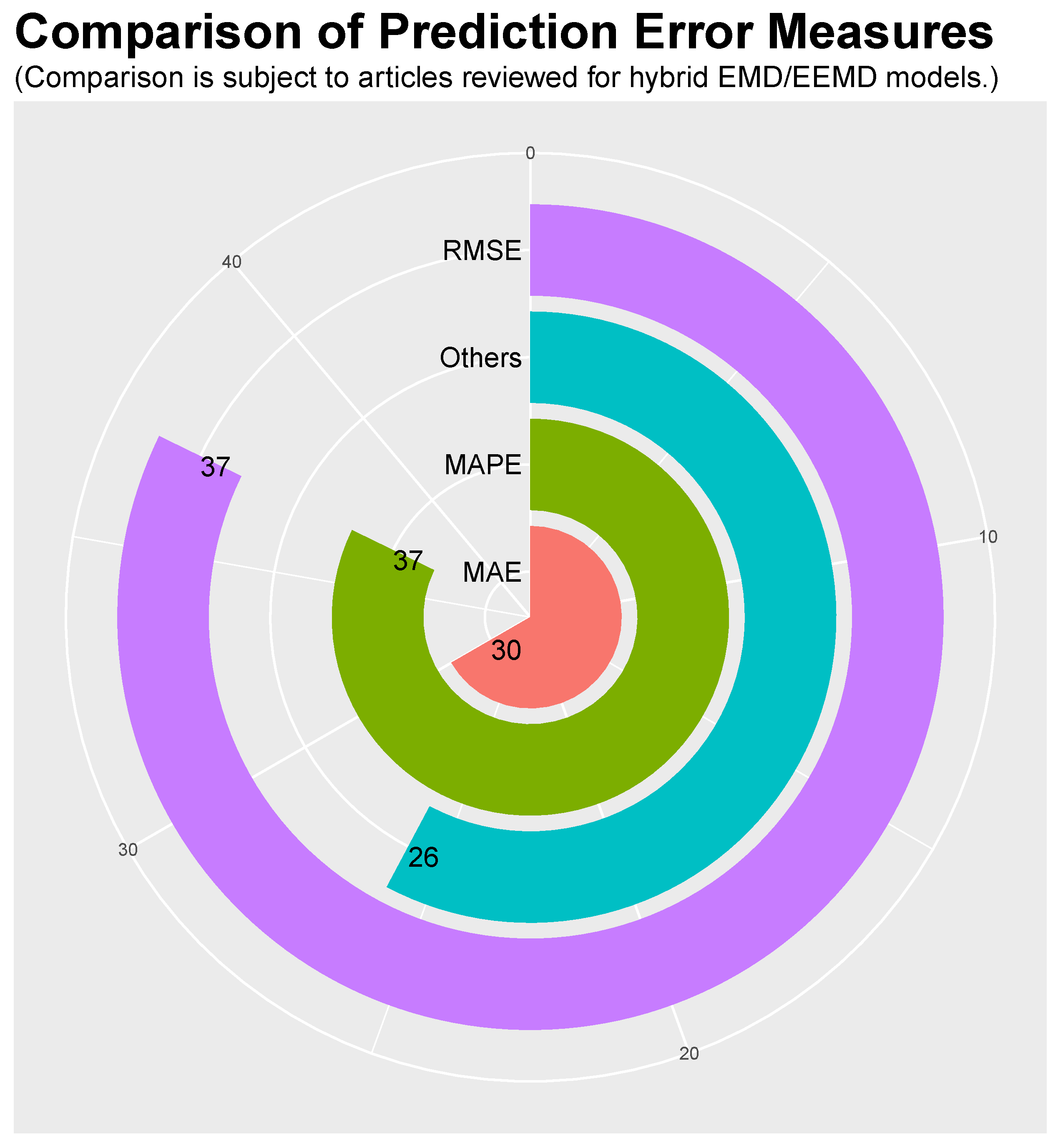
An et al. [30], Bao et al. [50], Wang et al. [44], Liu et al. [48], Sun et al. [43], Liu et al. [36], Liu et al. [55]
Liu et al. [49], Zhang et al. [14], Wu and Peng [41], Zhang et al. [28], Zhang et al. [46], Zhang et al. [12],
Yu et al. [37]
Xiaolan and Hui [59], Dejun et al. [60], Lin and Peng [18], Sun et al. [27], Sun and Yuan [39], Wang et al. [33],
Ren et al. [13], Wang et al. [32], Zang et al. [52], Wang et al. [15], Wang et al. [34], Zang et al. [52]
Guo et al. [10], Liu et al. [8], Zheng et al. [38], Hu et al. [19], Tatinati and Veluvolu [21],
Wang et al. [35], Sun and Liu [56]
Hong et al. [7], Zhang Xue-Qing [31], Liang et al. [58], Hong et al. [22], Safari et al. [42],
Jiang and Huang [40]
Ren and Suganthan [54], Ren and Suganthan [54], Zhang et al. [16], Ren et al. [11],
Drisya and Kumar [29]
Li and Wang [26], Jia [20], Fei [51]
Xingjie et al. [24], Dokur et al. [47]

