Abstract
The increasing energy demand and the changing of energy structure have imposed higher requirements on the conventional large-scale power plants control. Complexity of the power plant processes and the frequent change of operation condition make the accurate physical models hard to obtain for control design. To this end, a data-driven control strategy, the active disturbance rejection control (ADRC) has received much attention for the estimation and mitigation of uncertain dynamics beyond the canonical form of cascaded integrators. However, the robustness of ADRC is seldom discussed in a quantitative manner. In this study, the maximum sensitivity is used to evaluate and then constrain the robustness of ADRC applied to high-order processes. Firstly, by using the new idea of the vertical asymptote of the Nyquist curve, a preliminary one-parameter-tuning method is developed. Secondly, a quantitative relationship between the maximum sensitivity and the tuning parameter is established using optimization methods. Then, the feasibility and effectiveness of the proposed method is initially verified in the total air flow control of a power plant simulator. Finally, field tests on the secondary airflow control in a 330 MWe circulating fluidized bed confirm the merit of the proposed maximum sensitivity-constrained ADRC tuning.
1. Introduction
Power generation control remains a challenge problem due to the increasing electricity demand and the penetration of renewables—such as wind, solar, and tidal power—into a grid. To cope with the intermittency of renewable power, large-scale coal-fired power plants are required to operate under large and frequent variations. The performance of the air control system, one of the important control systems in the power plant, influences the whole plant safety and the energy efficiency. However, the accurate physical models of the power plant air systems are difficult to obtain because of the complicate combustion and heat transfer processes. In addition, the uncertainties brought by frequent variations impose higher control requirements in faster response and the ability to deal with disturbances. Therefore, a control strategy with strong ability in reference tracking and disturbance rejection is necessary for power plant air control systems. On one hand, it is preferred that the control strategy relies on accessible control input and output data instead of accurate process models. On the other hand, the robustness of the control system should be especially considered, as there are many sources of uncertainties and variations, such as variations in fuel quality, continuous change of working conditions, and other unknown disturbances.
Robustness is recognized as a ubiquitous system property in many fields ranging from biological systems and economics to computer science and control systems [1,2,3,4]. Robustness means that a system can handle uncertainty and remain effective under variations. There are many methods to evaluate the robustness level of a control system. For instance, µ-analysis [5] is considered a mature and efficient robustness analysis technique but it is difficult to calculate the structured singular value µ [6,7]. Monte Carlo methods have also been applied to measure performance robustness under random parameters variation [8,9,10]. Distribution of typical performance indices is presented when process parameters are randomly varied, but controller parameters remain unchanged. This image-based evaluation approach is very intuitive but lacks quantification to some extent.
The maximum sensitivity Ms was proposed as a single robustness index, which can limit the gain and phase margin simultaneously [11]. The relationship between maximum sensitivity Ms and gain and phase margin was clarified by Astrom and Hagglund [12]. It was then widely accepted as a robustness index in linear system control because it has a clear meaning and indicates the worst-case disturbance amplification of the disturbance. Most importantly, unlike other robustness indices, which are mainly used for analysis and evaluation, the maximum sensitivity Ms can also be used to instruct the controller design. Astrom and Hagglund [13] solved the non-convex optimization problem constrained by maximum sensitivity by finding the largest integral gain ki value on the envelopes generated by parameter boundaries. Yaniv and Nagurka [14] provided a series of equations for determining the proportional-integral-derivative (PID) controller parameters satisfying the sensitivity constraint. Alfaro and Vilanova [15] proposed a proportional-integral (PI) tuning method that achieved the desired maximum sensitivity by fitting techniques. Li et al. [16] applied the maximum sensitivity to tune the parameters of fractional internal model control (IMC)-PID controller. In this study, the maximum sensitivity is also employed to guide the controller design.
The concept of active disturbance rejection control (ADRC) [17,18,19] has attracted a lot of attention since the last decade. It is a data-driven control method, because the controller is designed by directly using input and output data without explicitly using the model information [20]. The key feature of ADRC is that it treats model uncertainties and external disturbances as a total disturbance to be estimated and compensated in real time. Since the interest in industry applications of data-driven ADRC has intensified in recent years [21,22,23,24,25,26,27,28,29,30], research interest in the industry implementation and related issues has also increased. Among the implementation issues [31,32], parameter tuning is a challenging task in process control, considering that high order dynamics, un-modeled dynamics, external disturbances and working condition variations are often present.
Optimization is one of the main methods for ADRC parameter tuning. Various algorithms such as the particle swarm optimization algorithm [33], reinforcement learning [34], and multi-objective optimization [35] have been used to tune the control parameters. However, because of the algorithm complexity and high computation cost, they are seldom implemented in industrial process control. The linear form of the ADRC and the bandwidth-tuning was firstly introduced by Gao [36]. It was then widely adopted by researchers and engineers because it allows a simpler formulation in the time domain and also provides additional insights into the frequency domain. Based on the bandwidth method, modifications have been made to improve the parameter tuning of the ADRC. Chen et al. [37] reduced the number of tuning parameters by specifying the desired closed loop dynamics. Tan and Fu [38] changed the ADRC into a two-degree-of-freedom internal model control (IMC) structure and suggested parameter tuning via IMC. Those methods are simple and effective for practical use but the robustness requirements are often not considered. Therefore, the main motivation of this study is to propose an effective and straightforward ADRC parameter tuning method that can satisfy the designed robustness level.
This study aims at deriving quantitative tuning rules for 1st-order ADRC that controls the typical high-order industrial processes under maximum sensitivity constraint. This is accomplished by firstly propounding a one-parameter-tuning rule and then establishing the quantitative relationship between the maximum sensitivity Ms and the tuning parameter. Experimental verification is performed for the total air flow control in a 1000 MWe coal-fired power plant simulator. Set-point tracking and disturbance rejection tests under constant and varying loads confirm the good performance and robustness of the proposed tuning method. Field tests are further conducted on the secondary air control in a 330 MWe in-service circulating fluidized bed (CFB). Field test results demonstrate the effectiveness and potential of the proposed maximum sensitivity-constrained ADRC tuning in industrial applications.
The main contributions of this study are: (i) a simple quantitative ADRC tuning method is proposed with the help of the asymptote of Nyquist curve, which is solved out for the first time; (ii) the desired maximum sensitivity is incorporated into the tuning formulas so that the proposed method can achieve certain robustness level with high precision; (iii) field tests in an in-service 330 MWe CFB unit verify the effectiveness and depict the potential of the proposed ADRC tuning method.
The paper is organized as follow: Section 2 formulates the problem. The quantitative ADRC tuning method is developed in Section 3. Section 4 initially demonstrates the feasibility of the proposed method via power plant simulator. After that, the ADRC control strategy and the proposed tuning method are implemented in an actual power plant in Section 5. Conclusions are drawn in Section 6.
2. Problem Statement
2.1. Processes Model
It is generally accepted that high-order models capture system behaviors with higher accuracy [39]. However, because of the mathematical difficulties in analyzing high-order processes, few studies on high-order processes have been conducted, in contrast to extensive studies on low-order processes or reduced order models. In fact, many industrial processes are of high order [40], such as the superheated steam temperature, main steam pressure, combustion system including the airflow system studied in this paper. Distributed parameter systems, which are common in power plant system, are inherently high-order. In addition, delay-dominated processes can be approximated to high-order processes. Meanwhile, few studies have addressed the parameter tuning of high-order processes. Therefore, in this study, the high-order process (1) is considered. It should be noted that all poles of the process model are considered to be the same for the simplicity of further development.
Because most industrial processes are non-oscillatory and self-regulatory, they can be modeled as described in Equation (1). Usually, the processes parameters n, T, K can be obtained through data-based modeling approach from the step-input test curve (known as the rising curve) and the data therefrom. Although the K/(Ts + 1)n-type model may not reflect all the characteristics of a real process, ADRC has the advantage of estimating and compensating total disturbance that includes modeling errors, so it can provide good control performance even when the identified high-order process does not have the exact model information.
2.2. First-Order Active Disturbance Rejection Control System
For the simplicity of implementation in the industrial distributed control system (DCS), the first-order data-driven ADRC controller is preferred in practice. The schematic diagram of the first-order linear ADRC is shown in the dashed box of Figure 1.
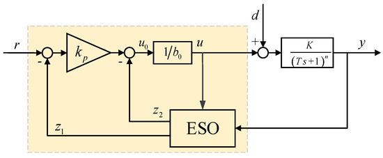
Figure 1.
Schematic diagram of the first-order linear ADRC.
The high-order process Gp(s) = K/(Ts + 1)n can be described by the following differential equations
where d is the external disturbances. Solve out for from (2) and defined and . The state-space representation of Gp(s) can be written as the following form
where parameter b0 is the designed control input gain. The term f is called the total disturbance, and it is extended as the second state x2. η represents the derivation of the total disturbance f. The total disturbance f includes the higher-order dynamics, parameter error and unknown external disturbance, which means it cannot be directly measured, thus it needs to be estimated or observed.
Based on Equation (3), a simple and low-order extended state observer (ESO) can be further designed.
In Equation (4), β1 and β2 are the observer gains. In the ESO, the states z1 and z2 estimate states x1 and x2, i.e., y and f, respectively. By compensating the estimated total disturbance z2 in real time,
the controlled process can be rewritten as
which means the process is compensated to become an integrating system. A simple feedback control can be designed on the compensated model.
In Equation (7), kp is the feedback controller parameter. The ESO output z1 is used as feedback signal instead of the measurement of y. The reason is that output z1 works as a filter for measurement y, so additional filter design is not required.
Combining (5), (6), and (7), the closed loop system has the approximated dynamics
From (3)~(8), it can be seen that a first-order linear ADRC controller has four parameters to tune, kp, β1, β2, and b0. Using the bandwidth-parameterization introduced by Gao [36], the number of the tuning parameters can be reduced to three, that is ɷc, ɷo, and b0, by
Moreover, by applying the singular perturbation theory [41], the stability of the first-order ADRC controlling high-order process can be proven mathematically. The stability analysis is provided in this study.
According to (3) and (4), the state-space representation of the process and ESO can be written in the form
where u is the control feedback law as described in (5) and (7). Then, denote e as the error of the feedback control loop and as the state estimation error of ESO. Also assume that the reference r is constant, so . With the bandwidth-parameterization in (9), the error dynamics of the first-order data-driven ADRC control system is
In order to transform the error dynamics into standard perturbation model, use the state transformation and let , so the first-order data-driven ADRC error dynamics can be rewritten as
where
In the standard perturbation form of error dynamic system (12), ε is called the singular parameter. When ωo is relatively large, ε is a small positive parameter. The error dynamic system can be considered as two parts: the state estimation error dynamics , which has fast response because the poles of ESO are relatively large, and the feedback control error dynamics , which has relatively slow response. The fast-and-slow characteristics of the error dynamic system constitute the basic feature of the singular perturbed system. Therefore, the singular perturbation theory is applied here to analyze the stability of the first-order data-driven ADRC control system.
Before giving the stability theorem, relative concepts about singular perturbation theory are introduced here. According to the singular perturbed theory, the standard singular perturbation model is
The quasi-steady-state solution can be obtained by letting .
The exact solution x, z can be described by the two-time-scale asymptotic expansions, where the quasi-steady term is defined in t-scale and the transient state is defined in -scale.
is called the boundary layer system and its dynamic behavior is
Then, the well-known fundamental theorem [42] in singular perturbation methods is presented.
Assumption 1.
The equilibrium of the boundary layer system is asymptotically stable uniformly in x0 and t0, and belongs to its domain of attraction.
Assumption 2.
The eigenvalues of have real parts smaller than a fixed negative number for , along , i.e., .
Theorem 1.
If Assumption 1 and 2 are satisfied, them , then the approximation and are valid for all , and there exists such that .
Then, the stability properties of the data-driven ADRC error dynamic system (12) can be obtained easily by applying the above theorem. Write the first-order data-driven ADRC error dynamics in the standard singular perturbation form
So, the quasi-steady-state solution is
and the boundary layer system is
The equilibrium of the boundary layer system is and it is asymptotically stable uniformly in e0 and t0. Because the boundary layer system (20) is linear and the matrix AZ is Hurwitz, so the equilibrium is globally asymptotically stable. So it is obvious that belongs to the attraction domain. Assumption 1 is satisfied.
For , along , , so Assumption 2 is satisfied.
Therefore, and are valid for all , and there exists such that . Since , exists for . For , since and matrix is Hurwitz considering , so is asymptotically stable and , so .
In the above deduction, in order to ensure that is a small positive parameter, so is positive and it is relatively large. In sum, with the use of the bandwidth-parameterization, there exists and such that the first-order data-driven ADRC error dynamic system (12) is uniformly asymptotically stable.
2.3. Maximum Sensitivity
The maximum sensitivity Ms is defined as the maximum value of the sensitivity function among the frequency range. The maximum sensitivity Ms can be seen as the worst-case amplification of disturbances, and a reasonable range of Ms for control design is 1.0–2.5 [12].
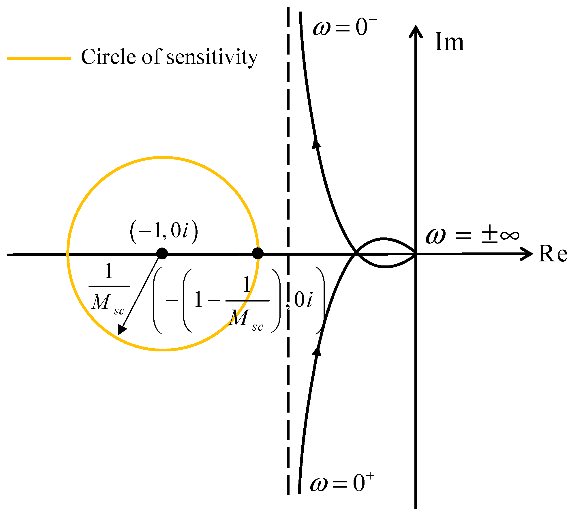
In the definition of the maximum sensitivity, Equation (21), Gl(iɷ) is the frequency characteristic of the open-loop transfer function. The maximum sensitivity Ms can be graphically interpreted as the inverse of the shortest distance from the Nyquist curve to the critical point (−1,0i).
Because the maximum sensitivity Ms is closely related to the open-loop transfer function Gl(s), the function Gl(s) of the first-order ADRC controlling the high-order processes is necessary for further analysis. It can be easily obtained from the two-degree-of-freedom control configuration of ADRC [31].
Combining Equations (21) and (22) results in
3. Derivation of Parameter Tuning Formulas
As stated in Section 1, this study aims at developing a quantitative tuning rule that can provide a desired robustness level. This is achieved by initially deriving an analytical tuning rule with one parameter to tune. Subsequently, optimization methods are applied to provide the relationship between the maximum sensitivity Ms and the tuning parameter.
3.1. One-Parameter-Tuning Method
It is always difficult to directly obtain tuning parameters from Equation (23) because of the strong nonlinearity and the high-order characteristics of process model. It is highly nonlinear because of the absolute value operation. In addition, it is at least fifth-degree, which makes it almost impossible to obtain an explicit solution. However, in this study, this problem is tackled from a different perspective.
If a certain maximum sensitivity constraint Msc is given, a circle of sensitivity centered at (−1,0i) with the radius 1/Msc, can be constructed. As shown in Figure 2, if the Nyquist curve of Gl(iɷ) does not enter the circle of sensitivity, it means that the shortest distance from the Nyquist curve to the point (−1,0i) is larger than 1/Msc; therefore, the real maximum sensitivity is smaller than Msc.
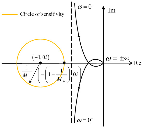
Figure 2.
Schematic diagram of the first-order linear ADRC.
Based on the graphical interpretation, deriving the tuning parameters under a maximum sensitivity constraint is equivalent to finding the parameters with the Nyquist curve outside the circle of sensitivity. Fortunately, a vertical asymptote is discovered in the Nyquist curve of Gl(iɷ), which is typical for this type of controlled high-order processes. An alternative condition for satisfying the maximum sensitivity constraint is further proposed: the asymptote of the Nyquist curve of Gl(iɷ) should be located to the right side of the circle of sensitivity, so the Nyquist curve does not enter the sensitivity circle.
The following part will show the deduction of the asymptote function and how the asymptote condition is used to guide the derivation of the parameter tuning method.
Return to the ADRC parameters. In the bandwidth-parameterization, ɷc equals kp; therefore, it influences the desired closed-loop dynamics. Let the desired settling time be ts* = knT, where k is the desired settling time factor. Chen et al. [37] proposed ɷc = 10/ts* for the second-order ADRC. By applying this to the first-order ADRC parameter tuning,
Parameter ɷo denotes the ESO bandwidth. Generally, it determines how fast the ESO can estimate and cancel the total disturbance. A recommended choice for ɷo [36] is
By combining Equations (9) and (25) and rewriting Equation (22), the frequency description of the open-loop transfer function is obtained
According to Figure 2, the Nyquist curve of Gl(iɷ) approaches the asymptote line when ɷ → ±0, so the limiting values of Gl(iɷ) is of concern. Let
where
When ɷ → 0−, , and p1 → 1, p2 → nTɷ. Then,
Similarly, when ɷ → 0+,
This result verifies that the asymptote is vertical and its function is
As shown in Figure 2, the rightmost point of the circle of sensitivity is (−(1 − 1/Msc),0i). Let the asymptote is on the right side of the sensitivity circle, then
According to Equation (23), increasing b0 can reduce the maximum sensitivity Ms. For the purpose of a conservative design, let b0 be 1.4 times the low limit and the maximum allowable value of the sensitivity constraint is used, Msc = 2.5. Then,
So far, the preliminary tuning formulas of the first-order ADRC applied to the high-order processes are
It is a one-parameter-tuning rule, where the desired settling time factor k is the tuning parameter for the trade-off between performance and robustness. Since the sign of b0 should be the same as the sign of the process gain K [43], a reasonable range of k can be determined from Equation (33), k = 1~7.
3.2. Relationship between Maximum Sensitivity and Tuning Parameter
Because of the conservativeness in the previous design, the tuning formulas in Equation (34) usually result in a lower maximum sensitivity than Msc = 2.5. In this section, the relationship between the tuning parameter k and the real maximum sensitivity Ms is found. Users can then specify the system robustness level by using Ms as a tuning parameter.
Substituting Equations (26) and (34) into Equation (21) provides the expression of maximum sensitivity
It can be seen from the expression that the process gain K does not influence Ms any more, while the desired settling time factor k, the process order n, and the process time constant T are still related to Ms.
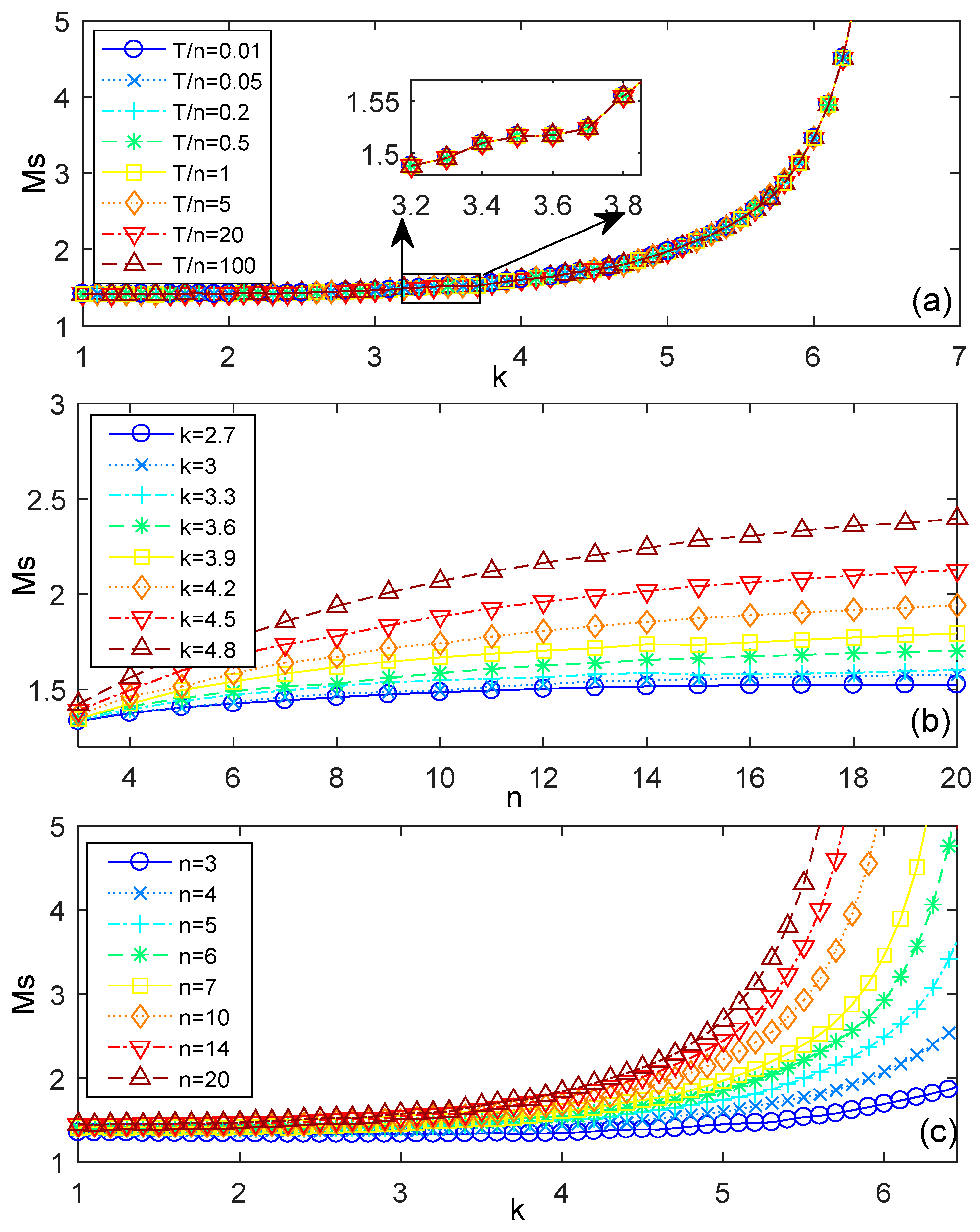
Simulations have been performed to test how T, n, and k influence Ms in the range of T/n = 0.01~100, n = 3~20, k = 1~7. The results are plotted in Figure 3.
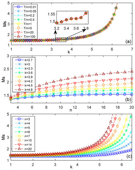
Figure 3.
Influence of n, T, and k on Ms. (a) Ms changes with k under different T/n, when n = 7, K = 1; (b) Ms changes with n under different k, when T/n = 7, K = 1; (c) Ms changes with k under different n, when T/n = 1/15, K = 1.
Figure 3a shows that the curves of different T/n ratio coincide, which indicates that the process time constant T has no influence on the maximum sensitivity Ms. This occurs because T and ω appear in pairs in Equation (35). It means that T is a scaling of frequency ω, so it does not affect the shape of the Nyquist curve and thus does not affect the value of maximum sensitivity Ms. Figure 3b,c also show that Ms changes with n logarithmically and changes with k exponentially. Therefore, we propose that
Solve for k, which gives
Equation (37) calculates a certain k to ensure that the system’s robustness level at Ms. By using nonlinear fitting techniques, the coefficients a1, a2, and a3 will be further determined.
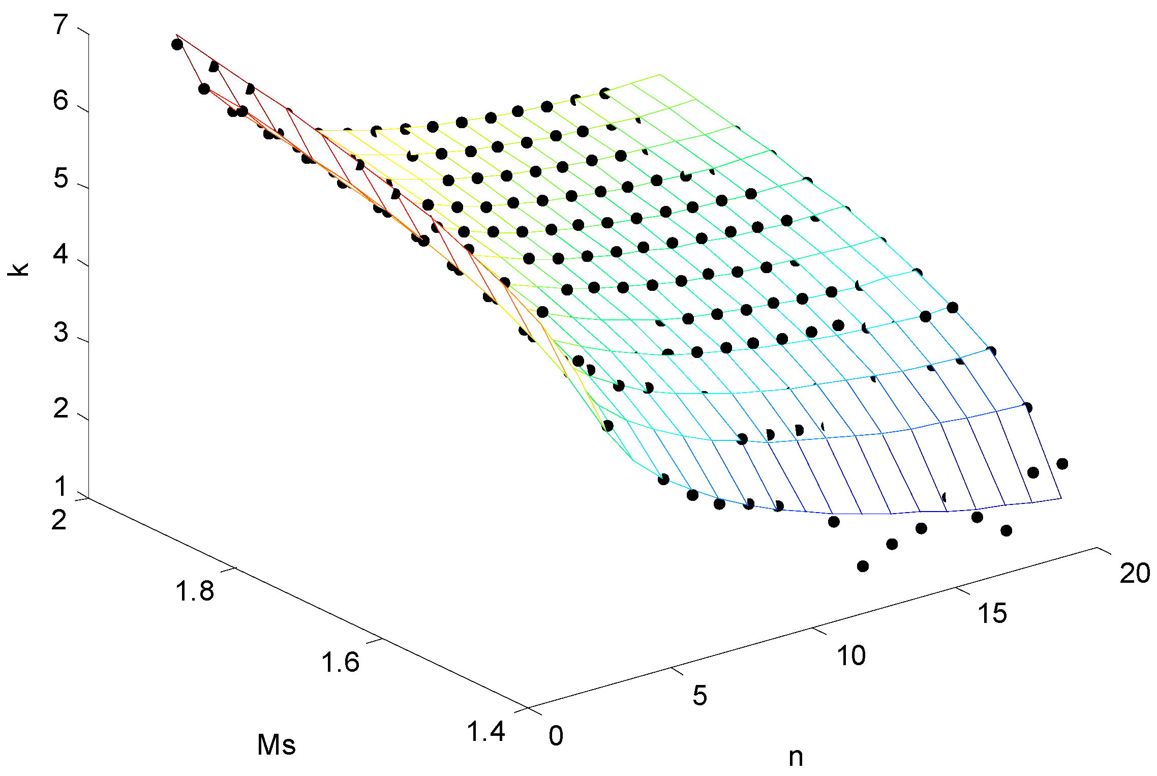
First, the data sets Ms, n, and k are required for fitting. For Ms = 1.4~2.0, n = 3~20, the data set of k can be generated by minimizing the integrated absolute error (IAE) of reference tracking and disturbance rejection response.
A dataset of k was therefore determined (see dots in Figure 4). Nonlinear fitting gives the estimation of coefficients a1 = 1.3966, a2 = 0.0026, a3 = 1.6980 with an average error E = 0.165 and a variance S = 0.0252. To improve the fitting precision, the regression model for fitting is modified as
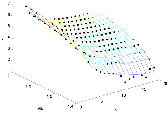
Figure 4.
Multivariable fitting of k. Dots represent the fitting data set and the mesh represent the fitting results.
Thus, the corresponding estimated coefficients are
which gives an average fitting error E = 0.047 and a fitting variance S = 0.0055. The fitting result is shown in Figure 4.
To sum up, for a high-order process, K/(Ts + 1)n, if a designed maximum sensitivity (1.4~2.0) is given for the controller design, then the first-order ADRC parameters can be calculated through the following equations.
3.3. Illustrative Example
The following simulation example will show how the choice of the designed maximum sensitivity influences the control performance and robustness. It will also demonstrate that the proposed tuning formulas can ensure the actual maximum sensitivity Ms of the controlled system achieves the designed maximum sensitivity with good accuracy. Consider a process
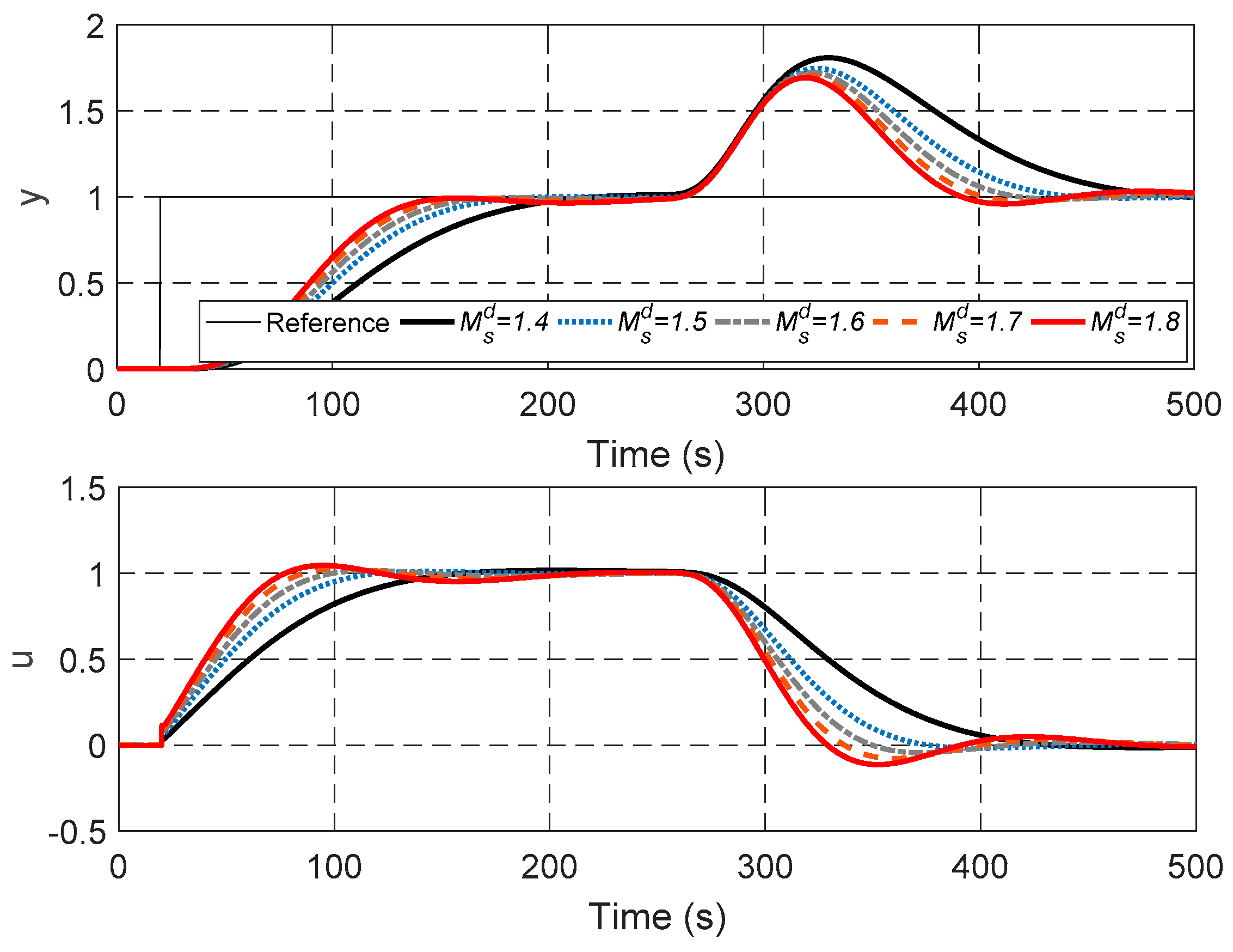
let the designed maximum sensitivity be 1.4, 1.5, 1.6, 1.7, and 1.8. Several sets of parameters with different robustness levels are thus calculated from Equation (41). Simulations are performed by MATLAB Simulink R2016b. Simulations are configured as fix-step type with a step size of 0.1 s, and the Euler integration method is chosen as the solver algorithm. The output response with a unit step reference at t = 20 s and a unit step disturbance at t = 250 s is shown in Figure 5. The Nyquist plots are depicted in Figure 6. The controller parameters and control performance indices are listed in Table 1. Ts and σ are settling time (under 5% standard) and overshoot. The control performance indices the integral absolute error (IAE), the total variation (TV), and the integral of the time-weighted absolute error (ITAE) used in this study are defined in Equation (43). In (43), te and h are the simulation time and step size.
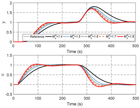
Figure 5.
Output responses for different values of the designed maximum sensitivity .
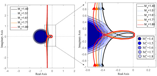
Figure 6.
Achieved maximum sensitivity Ms and designed maximum sensitivity .

Table 1.
ADRC controller parameters and performance indices under different designed maximum sensitivity for G(s) = 1/(10s + 1)5.
Figure 5 shows that a higher designed maximum sensitivity results in a faster response to the set point tracking and the disturbance rejection. At the same time, a higher designed maximum sensitivity may result in oscillation, which should be regarded as an indication of decreased robustness.
To be more specific, a higher designed maximum sensitivity results in a smaller b0, as shown in Table 1, which means a bigger amplification of the feedback output. That explains the faster response and the smaller IAE. In addition, Table 1 also shows that increasing results in an increase in TV of the control input. The TV can be regarded as an indication of the control efforts and the wear of the actuators. It should especially be of concern when evaluating the economic performance of the control system. Thus, the trade-off between performance, robustness, and cost should be carefully considered when control is applied in a practical scenario.
The Nyquist plots are depicted in Figure 6. The left figure shows that the Nyquist curves of different robustness level converge to a vertical asymptote. The right figure is the enlarged view of the left figure, showing the agreement between the real maximum sensitivity Ms and the designed maximum sensitivity . The circles layered with different colors are the circles of sensitivity, representing different designed maximum sensitivity . The Nyquist curves are almost tangential to each of the circles, implying that the proposed tuning method is indeed able to yield a specified robustness level.
Furthermore, the stability analysis in Section 2.2 can be applied in this simulation example. In the proposed tuning Formulas (41), the value of is 10 times as , which enables the ADRC control system to own fast-and-slow characteristics. The initial values of the ESO states are kept as default in Simulink, which means the initial tracking errors , so . However, because the equilibrium is globally stable, still belongs to the attraction domain. It is obvious that , and , therefore, Assumptions 1 and 2 are satisfied and the data-driven ADRC control system has asymptotical stability. The simulation results of process (42) validate the stability of this data-driven ADRC control system.
In addition, the proposed tuning method based on the high-order process can also be applied to other types of processes if they can be approximated to the form of K/(Ts + 1)n. However, the proposed tuning method cannot ensure the achievement of the designed maximum sensitivity for other types of processes. Since the purpose of this study is to derive a tuning method that can achieve the designed maximum sensitivity, a discussion on the application to other types of processes is not included in this paper.
4. Experimental Validation on Power Plant Simulator
To validate the effectiveness of the proposed maximum sensitivity-constrained tuning method, the method is tested on the total airflow control in a 1000 MWe coal-fired power plant simulator. The simulator and the control systems are constructed on a software named Industry Automation Platform (IAP). The calculation step size used in the simulator experiments is 0.1 s, and the data collection step size is 1 s.
Excessive or inadequate airflow may decrease the combustion efficiency, or even threaten the combustion stability in the furnace. For this reason, the airflow should be maintained at an optimal value. In the DCS, the airflow set-point value (SV) is decided by the boiler master demand and fuel feed. Based on the difference between the SV and the measured airflow (or process value (PV)), ADRC algorithm gives commands to the forced draft fans to adjust the pitch blade position (scaled in permillage), which is the manipulated value (MV) of this control system.
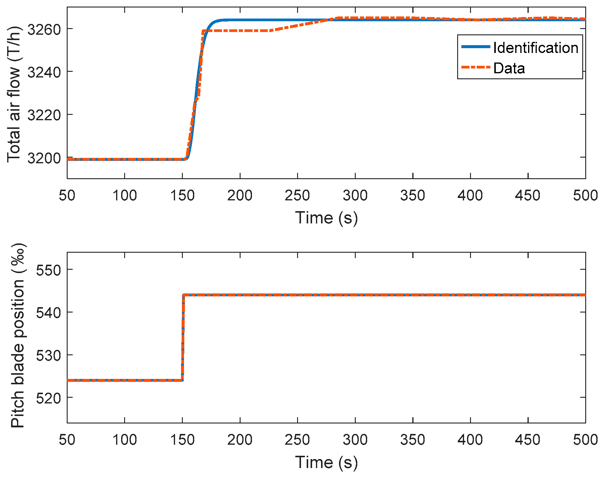
By using data-based modeling, the dynamic from the forced draft fans to the total airflow is determined from open-loop step test data. In order to apply the proposed ADRC tuning method, the total airflow process is identified to the K/(Ts + 1)n-type process. The model parameters K and T are identified by the Simulink parameter estimation tool. The optimization method is nonlinear least squares. The model order n is decided by choosing the identified model with the lowest cost function value. The identified result is presented in Equation (44) and Figure 7. Although the identified simple high-order process cannot capture all the complex dynamics of the total air process, the ability of ADRC in estimating and compensating the un-modeled dynamics enables ADRC to provide good control results for complex industrial processes.
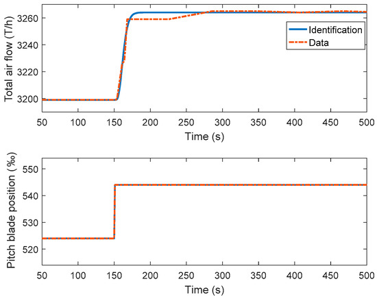
Figure 7.
Open loop identification of the total air flow control process.
The first-order ADRC algorithm is implemented in the 1000 MWe power plant simulator by using IAP configuration software. Typical modules used are math operation, integrating module and Boolean logical operation. Before testing the proposed ADRC method in the power plant simulator DCS, MATLAB simulations were conducted based on this model to generate suitable parameters. According to Equation (44), the process gain K, time constant T and order n are 3.25, 2.433, and 5, respectively. The only tuning parameter, namely the designed maximum sensitivity , is set as 1.4 to achieve a moderate robustness level. With process parameters n, T, K and the tuning parameter known, the first order ADRC parameters ωc, ωo, and b0 can be calculated by the proposed tuning equations in (41). PI controller used in the total airflow control loop is retuned to achieve the same maximum sensitivity as that in the ADRC tuning. The retuning of PI parameters is accomplished through optimization. Since only IAE or ITAE index used as objective function leads to PI parameters with high overshoot in tracking performance, the objective function is a combination of ITAE and overshoot indices. The optimization constraint is that maximum sensitivity Ms = 1.4, and the optimization algorithm used is the sequential quadratic programming.
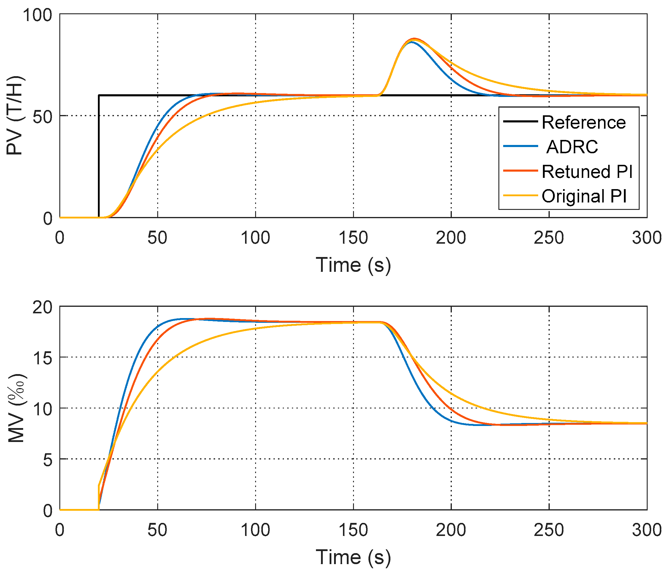
Figure 8 shows the simulation results of the different control and tuning strategies on MATLAB. Table 2 lists the parameters and performance indices. The original PI parameters result in a relative slow response because of the conservative tuning. The retuned PI parameters achieve a maximum sensitivity of 1.4 and it has improved the control performance a lot. The proposed ADRC tuning method results in the real maximum sensitivity Ms = 1.407, which is very close to the designed value = 1.4.
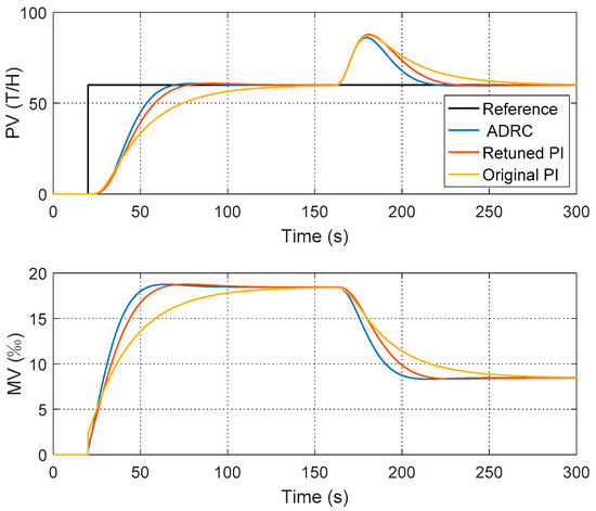
Figure 8.
Comparative simulations based on the identified model.

Table 2.
Controller parameter settings, performance, and robustness indices for the total air control.
Figure 9 shows the experimental results in the power plant simulator. Experiments are carried out under a constant load of 1000 MWe. The set-point is changed from 3100 T/h to 3200 T/h and a 10‰ pitch blade disturbance lasting about 500 s is added to the system around 1100 s. Experiment results show agreement with the simulation. The retuned PI has improved the control performance of the original PI. The ADRC shows control advantages in set-point tracking and disturbance rejection.
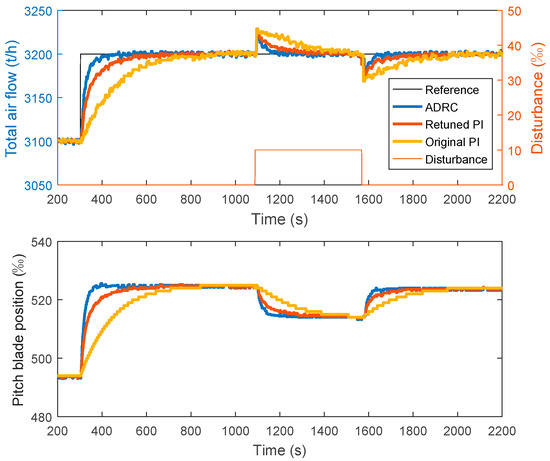
Figure 9.
Set-point tracking and disturbance rejection tests of the total airflow control.
Since the total airflow control is closely related to the power plant load, the system dynamics vary with the operating conditions. It is necessary to test different controllers under varying loads. Figure 10 shows that the proposed ADRC tuning method still maintains good tracking performance when the load changes from 700 MWe to 1000 MWe.
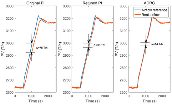
Figure 10.
Reference tracking under varying loads.
In Table 3, the average settling time , overshoot σ under constant load condition, the average tracking error under varying load condition have been calculated for different control strategies. It can be seen that the average settling time and the average tracking error of ADRC control strategy have been remarkably reduced by about 50%, compared to the retuned PI control. The overshoot σ during disturbance rejection has also been decreased by 5.7%.

Table 3.
Control performance comparison in the total air control experiments under constant and varying load.
The experimental tests in a coal-fired power plant simulator initially demonstrate the feasibility of the proposed maximum-constrained maximum sensitivity tuning method. It not only provides satisfactory control performance in set-point tracking and disturbance rejection, but also shows the good robustness under varying working conditions.
5. Field Test on Secondary Air Control in Actual Power Plant
Although the power plant simulator contains the same control system a real power plant, it is not realistic enough to reflect all the characteristics of a real power plant. The control of actual industrial processes is more challenging, especially when unknown multi-source disturbances are often present. To strengthen the conclusions made in Section 4, the proposed ADRC tuning method is further applied to an actual industrial process. The ADRC control algorithm and the tuning method are applied to the secondary air control system of a 330 MWe circulating fluidized bed (CFB) unit, which is in commercial operation in the Shanxi Province in China.
5.1. Process Description
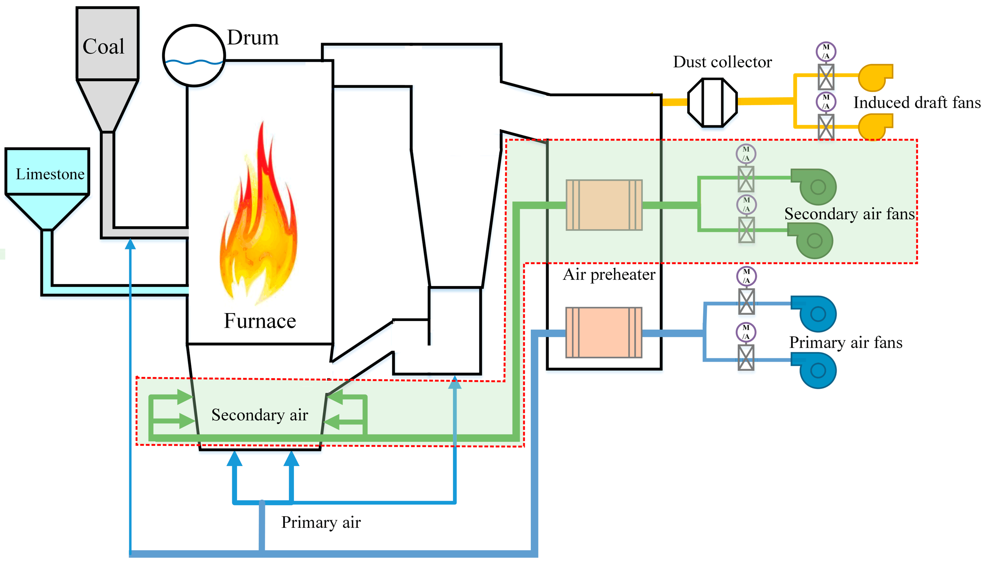
A combustion system is an essential part of a CFB unit. It is the place where fuel and air are mixed, and the chemical energy of the fuel is converted into thermal energy to heat the working fluid. Compared to a pulverized coal-fired boiler, the solid materials in a CFB boiler must be fluidized and circulated by air, making the combustion air system of a CFB boiler more complicated. Figure 11 shows the schematic diagram of the air and smoke system in the CFB unit. The high-pressure blowers supply high-pressure air to fluidize and overflow the bed material in a loop seal. Primary air fans supply hot primary air upwardly into the furnace to fluidize the solid particles. At the same time, a small proportion of the primary air is sent to the coal feeding system as spreading air. The secondary air fans convey the secondary air to the interface between the lower and upper zone of the furnace, constituting 20–60% of the total air. The secondary air is added to the furnace to create an oxygen-rich environment, which improves the combustion efficiency.
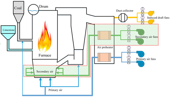
Figure 11.
Configuration diagram of the air and smoke system in a CFB unit.
Because the failure of controlling the primary air and the loop seal air can severely damage the normal fluidization and circulation state of the CFB boiler, while the control of the secondary air system mainly influences the combustion efficiency, so it is less risky to test the ADRC tuning on the secondary air system in a commercially operated power plant. Therefore, for safety considerations, the secondary air system is chosen for the field test.
The ADRC algorithm is implemented in the SUPCON DCS in parallel with the original PID algorithm. Implemental issues such as the bumpless transfer between the PID, ADRC, and manual mode, as well as the amplification limit and rate limit, have been carefully solved. The schematic diagram of the control system is shown in Figure 12. The balance module receives control commands from PID or ADRC controller and distributes the control commands to each secondary air fan. Under normal conditions, the control command is equally distributed to the two air fans. If the working efficiency of the two fans changes, the operators can add an offset to the balance module to even out the power output of the two air fans.

Figure 12.
Schematic diagram of the secondary air control system.
5.2. Process Identification
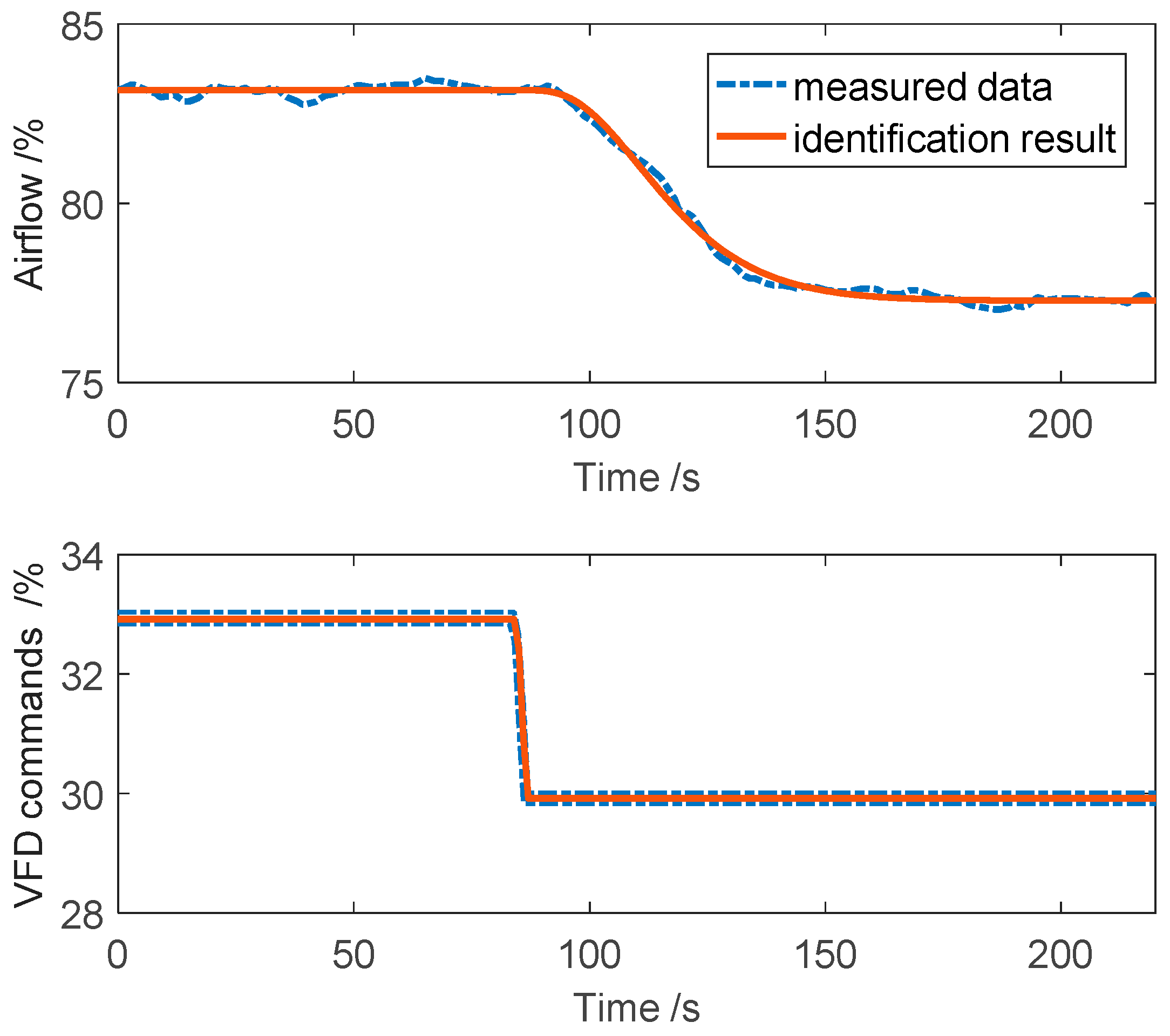
The secondary air flow, scaled in percentage, is controlled by the variable frequency drive (VFD) attached to the air fan motors. The VFD commands are the control input, which is also scaled in percentage. In order to use the proposed ADRC tuning method to determine appropriate controller parameters, the input-step experiment data are collected for identification purposes. Same data-based modeling method is used as it in the total air identification. The identification results are shown in Figure 13 and the transfer function is given in Equation (45).
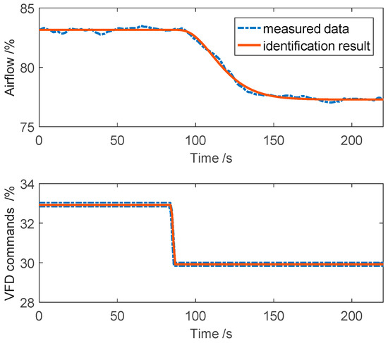
Figure 13.
Identification of the secondary air flow control system.
5.3. Process Identification
In Equation (45), the secondary air control process is identified into a K/(Ts + 1)n-type model, then the proposed ADRC tuning method is applicable. The process gain K, time constant T, and order n of the secondary process are 1.9596, 8.1874, and 4. Since the operation safety should be considered with special care. In the first test, a set of relatively conservative ADRC parameters are used. By setting the designed maximum sensitivity = 1.4, the initial ADRC parameters are calculated by using Equation (41). ADRC parameters ωc = 0.0969, ωo = 0.969, and b0 = 4.2721 are put in use. Please note that ADRC algorithm are in tracking mode when PID controller is working and the ADRC is switched on when the process is in steady state. During the control algorithm switch process, the bumpless transfer plays an important role here. Close observation is required after the first set of ADRC parameters are put in use. Only when no unstable oscillation or frequent control input variation occurs, further attempt is allowed. After ensuring the stability and robustness, another set of ADRC parameters with a faster response are calculated to improve the control performance. This is achieved by increasing the designed maximum sensitivity = 1.7. Similarly, the retuned ADRC parameters are calculated by the proposed tuning equation (41), and the obtained ADRC parameters are ωc = 0.0574, ωo = 0.5744, b0 = 0.9142. In addition, tests are also performed with the PID controller for comparison. The PID controller parameters are tuned by an experienced field engineer. The tuning process is based on prior knowledge and trial and error. The initial PI parameters are set as the same PI parameters from another CFB unit with similar capacity and configuration. The derivative part of PID controller is usually not used by engineers in power plant unit, because it may introduce noise to the control system and thus bring oscillation especially when the reference is frequently changed. The proportional gain Kp can be increased if faster set-point response is required, and it can be decreased if overshoot or oscillation appears. The integral gain Ki can be increased if the error elimination is slow, and the integral gain Ki also needs to be decreased when overshoot or oscillation happens. The final retuned PID controller parameters are decided with Kp = 0.3333, Ki = 0.0067, Kd = 0, which have been put in use for a long time to ensure enough robustness.
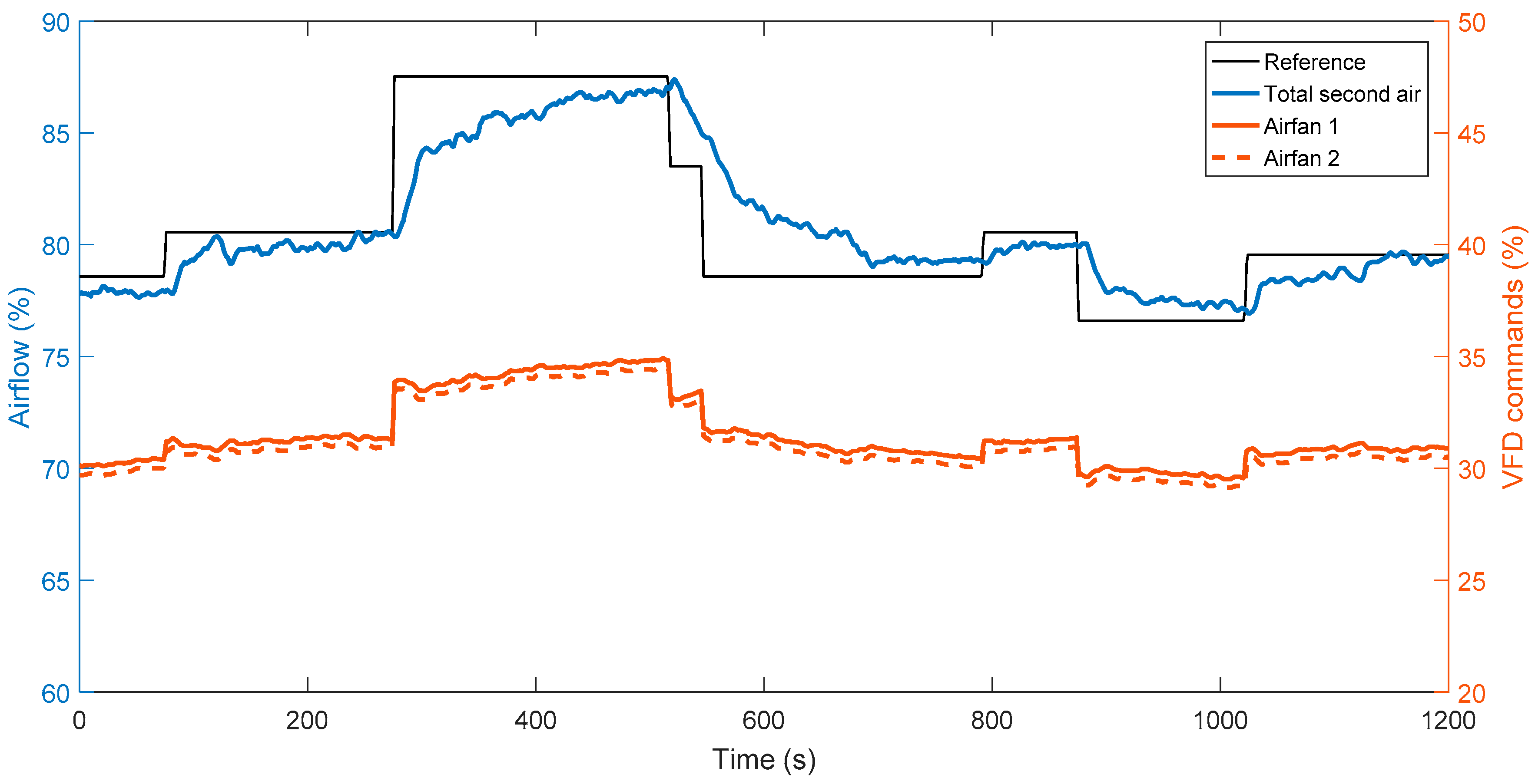
Reference tracking is the main concern for a secondary air control system, because the secondary air flow must rapidly respond to the varying load reference of the CFB unit. Therefore, the air flow reference is step-changed for performance tests. In addition, artificial disturbances are not allowed for this commercially operated power plant, so strict disturbance rejection tests are therefore excluded. For a fair comparison, reference step tests for the ADRC and PID are performed within the same load range of 230~240 MWe. The test results of 20-min period are shown in Figure 14 and Figure 15. The control performance indices including the average settling time , the IAE, ITAE, and the average total variation of two air fans are summarized in Table 4.
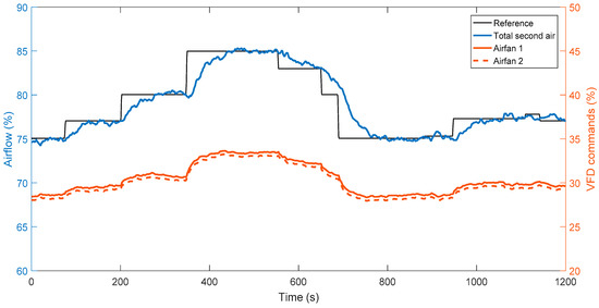
Figure 14.
Reference step test results of the ADRC in the CFB unit (time span of test: 1 September 2017, 9:28:50–9:48:50).
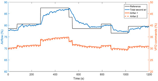
Figure 15.
Reference step test results of the PID in the CFB unit (time span of test: 1 September 2017, 9:55:30–10:15:30).

Table 4.
Control performance comparison of ADRC and PID in the secondary air control system of a 330 MWe in-service CFB unit.
It can be seen from Table 4 that the average settling time , IAE and ITAE indices have been reduced by more than 40% under the proposed ADRC tuning method, which means the proposed ADRC tuning has provided a better reference tracking. In the meanwhile, the average total variation of the control input has also been reduced by 18.5%. A reduction in TV indicates less frequent position changes of the fan blades, which means less tear and wear of the air fans, thus the maintenance cost could be reduced.
In addition, the stability analysis can also be applied to the two validation tests for airflow control. Similar to stability analysis of the simulation example in Section 3.3, using the proposed ADRC tuning method (41) ensures and is relatively large. The difference from the simulation example is that the initial values of ESO in validation tests are not set as 0. In the industrial practice, the data-driven ADRC algorithm is implemented in parallel with PID control algorithm. The ADRC is designed to operate under tracking mode when PID controller is in use. For safety consideration, the ADRC is usually switched on and put into use when the process is in steady state. In this case, the initial ESO tracking errors , so and it belongs to the attraction domain. Hence, Assumptions 1 and 2 are satisfied. The data-driven ADRC controls airflow systems have asymptotical stability and its stability is validated with experimental and test results.
It can be concluded that the proposed maximum sensitivity ADRC tuning improved the control performance. The explicit form of the tuning equations facilitates the calculation of the ADRC parameters. The maximum sensitivity-constrained tuning that provides the desired robustness allows for a safer implementation of the control algorithm. The field test results show that the proposed ADRC tuning method has the potential for further industrial applications.
6. Conclusions
In this paper, the data-driven ADRC control strategy is studied for industrial processes. This study achieves the goal of deriving maximum sensitivity-constrained tuning formulas for first-order ADRC.
To sum up, the proposed maximum sensitivity constrained ADRC tuning method has the following advantages: (i) The proposed tuning equations are explicit and simple, so the data-driven ADRC parameters can be easily obtained without complex programming and calculation. (ii) The tuning process is easy. The designed maximum sensitivity is the only tuning parameter, thus it requires little tuning workload. (iii) The proposed ADRC tuning method can achieve the designed maximum sensitivity with high accuracy, which allows the controlled system with designed robustness level. The disadvantage of the proposed ADRC tuning method is that it does not apply to non-self-regulating processes, such as integrating processes and unstable processes. Parameter tuning towards non-self-regulating processes can be future research topics.
The experimental results on the total air flow control in the power plant simulator demonstrate that the proposed method has advantages in reference tracking and disturbance rejection. The field tests on the secondary air control in the in-service CFB unit reveal a promising prospect of the proposed ADRC tuning method in industrial process control. Future work will be focused on more industrial applications of this maximum sensitivity-constrained ADRC tuning method.
Author Contributions
Conceptualization, T.H.; Funding acquisition, L.W. and D.L.; Methodology, T.H., D.L. and L.S.; Project administration, D.L. and L.W.; Resources, L.W. and S.Z.; Software, S.Z.; Supervision, D.L.; Validation, T.H. and Z.W.; Writing—original draft, T.H.; Writing—review & editing, T.H., Z.W., R.S., D.L. and L.S.
Funding
This study was funded by the National Key Research and Development Program of China, 2016YFB0901405. This study also receives financial support from the State Key Lab of Power Systems, Tsinghua University.
Acknowledgments
The authors want to thank the technical support of the IAP platform provided by Jingshu Guo, Wang Zhang, and Weimin Huang. The authors also would like to thank Fengsheng Jia, Haisu Wu, and his colleague, and Lei Han for their technical and administrative support during field tests in Shangxi Province.
Conflicts of Interest
The authors declare no conflict of interest.
References
- Hiroaki, K. Biological robustness. Nat. Rev. Genet. 2004, 5, 826–837. [Google Scholar]
- Xun, L.; Halbert, W. Robustness checks and robustness tests in applied economics. J. Econ. 2014, 178, 194–206. [Google Scholar]
- Femandez, J.C.; Mounier, L.; Pachon, C. A model-based approach for robustness testing. In Proceedings of the IFIP International Conference on Testing of Communicating System, Montreal, Canada, 31 May–2 June 2005; Springer: Berlin/Heidelberg, Germany; pp. 333–348. [Google Scholar]
- Zames, G. Feedback and optimal sensitivity: Model reference transformations, multiplicative seminorms, and approximate inverses. IEEE Trans. Autom. Control 1981, 26, 301–320. [Google Scholar] [CrossRef]
- Doyle, J. Analysis of feedback systems with structured uncertainties. IEE Proc. D-Control Theor. Appl. 1998, 192, 242–250. [Google Scholar] [CrossRef]
- Braatz, R.; Young, P.; Doyle, J.; Morari, M. Computational complexity of µ calculation. IEEE Trans. Autom. Control 1994, 39, 1000–1002. [Google Scholar] [CrossRef]
- Lesprier, J.; Roos, C.; Biannic, J.; Morari, M. Improved µ upper bound computation using the µ-sensitivities. IFAC-PaperOnLine 2015, 48, 215–220. [Google Scholar] [CrossRef]
- Laura, R.R.; Robert, F.S. A monte carlo approach to the analysis of control system robustness. Automatica 1993, 29, 229–236. [Google Scholar]
- Zhang, Y.; Li, D.; Gao, Z.; Zheng, Q. On oscillation reduction in feedback control for processes with uncertain dead time and internal-external disturbances. ISA Trans. 2015, 59, 29–38. [Google Scholar] [CrossRef]
- He, T.; Li, D.; Wu, Z.; Xue, Y.; Yang, Y. A modified luenberger observer for SOC estimation of lithium-ion battery. In Proceeding of the 36th Chinese Control Conference, Dalian, China, 26–29 July 2017; pp. 924–928. [Google Scholar]
- Persson, P.; Astrom, K.J. Dominant pole design—A unified view of PID controller tuning. Processing of the 4th IFAC Symposium on Adaptive System in Control and Signal, Grenoble, France, 1–3 July 1992; pp. 127–132. [Google Scholar]
- Astrom, K.J.; Hagglund, T. Advanced PID Control; ISA Press Research Triangle Park: Durham, NC, USA, 2006; pp. 111–117. [Google Scholar]
- Astrom, K.J.; Hagglund, T. Design of PI controllers based on non-convex optimization. Automatica 1998, 34, 565–601. [Google Scholar] [CrossRef]
- Yaniv, O.; Nagurka, M. Design of PID controllers satisfying gain margin and sensitivity constraints on a set of plants. Automatica 2004, 40, 111–116. [Google Scholar] [CrossRef]
- Alfaro, V.; Vilanova, R. Model-reference robust tuning of 2DoF PI controllers for first- and second-order plus dead-time controlled processes. J. Process Control 2012, 22, 359–374. [Google Scholar] [CrossRef]
- Li, D.; Liu, L.; Jin, Q.; Hirasawa, K. Maximum sensitivity based fractional IMC-PID controller design for non-integer order system with time delay. J. Process Control 2015, 31, 17–29. [Google Scholar] [CrossRef]
- Han, J. From PID to active disturbance rejection control. IEEE Trans. Ind. Electron 2009, 56, 900–906. [Google Scholar] [CrossRef]
- Gao, Z. Active disturbance rejection control: From an enduring idea to an emerging technology. In Proceedings of the 2015 10th International Workshop on Robot Motion and Control, Poznan, Poland, 6–8 July 2015; pp. 269–282. [Google Scholar]
- Xue, W.; Huang, Y. Performance analysis of active disturbance rejection tracking control for a class of uncertain LTI systems. ISA Trans. 2015, 58, 133–154. [Google Scholar] [CrossRef] [PubMed]
- Hou, Z.; Gao, H.; Lewis, F.L. Data-Driven control and learning systems. IEEE Trans. Ind. Electron. 2017, 64, 4070–4075. [Google Scholar] [CrossRef]
- Han, J.; Wang, H.; Jiao, G.; Cui, L.; Wang, Y. Research on active disturbance rejection control technology of electromechanical actuators. Electronics 2018, 7, 174. [Google Scholar] [CrossRef]
- Roman, R.C.; Radac, M.B.; Tureac, C.; Precup, R.E. Data-Driven active disturbance rejection control of pendulum cart systems. In Proceedings of the Conference on Control Technology and Applications, Copenhagen, Denmark, 21–24 August 2018; pp. 933–938. [Google Scholar]
- Wang, G.; Xu, Q. Sliding mode control with disturbance rejection for piezoelectric nanopositioning control. In Proceedings of the Annual American Control Conference, Milwaukee, WI, USA, 27–29 June 2018; pp. 6144–6149. [Google Scholar]
- Sun, L.; Shen, J.; Hua, Q.; Lee, K.Y. Data-driven oxygen excess ratio control for proton exchange membrane fuel cell. Appl. Energy 2018, 231, 866–875. [Google Scholar] [CrossRef]
- Madoski, R.; Kordasz, M.; Sauer, P. Application of a disturbance-rejection controller for robotic-enhanced limb rehabilitation trainings. ISA Trans. 2014, 53, 899–908. [Google Scholar] [CrossRef]
- Ramirez, N.; Sira, R.; Garrido, M.; Luviano, J. Linear active disturbance rejection control of underactuated systems: The case of the furuta pendulum. ISA Trans. 2014, 53, 920–928. [Google Scholar] [CrossRef]
- Xue, W.; Bai, W.; Yang, S.; Song, K.; Huang, Y.; Xie, H. ADRC with adaptive extended state observer and its application to air-fuel ratio control in gasoline engines. IEEE Trans. Ind. Electron. 2015, 62, 5847–5857. [Google Scholar] [CrossRef]
- Fu, C.; Tan, W. Decentralized load frequency control for power systems with communication delays via active disturbance rejection. IET Gener. Trans. Distrib. 2018, 12, 1397–1403. [Google Scholar]
- Li, S.; Xia, C.; Zhou, X. Disturbance rejection control method for permanent magnet synchronous motor speed-regulation system. Mechatronics 2012, 22, 706–714. [Google Scholar] [CrossRef]
- Li, S.; Li, J. Output predictor-based active disturbance rejection control for a wind energy conversion system with PMSG. IEEE Access 2017, 5, 5205–5214. [Google Scholar] [CrossRef]
- Sun, L.; Li, D.; Hu, K.; Lee, K.Y.; Pan, F. On tuning and practical implementation of ADRC: A case study from a regenerative heater in a 1000 MW power plant. Ind. Eng. Chem. Res. 2016, 55, 6686–6695. [Google Scholar] [CrossRef]
- Gernot, H. Practical active disturbance rejection control: Bumpless transfer, rate limitation and incremental algorithm. IEEE Trans. Ind. Electron. 2016, 63, 1754–1762. [Google Scholar]
- Liu, Z.H.; Zhang, Y.J.; Zhang, J.; Wu, J.H. Active disturbance rejection control of a chaotic system based on immune binary-state particle swarm optimization algorithm. Acta Physica Sinica 2011, 60, 1–9. [Google Scholar]
- Wu, L.; Bao, H.; Du, J.; Wang, C. A learning algorithm for parameters of automatic disturbances rejection controller. Acta Automatica Sinica 2014, 40, 556–560. [Google Scholar]
- Sun, L.; Hua, Q.; Shen, J.; Xue, Y.; Li, D.; Lee, K.Y. Multi-objective optimization for advanced superheater steam temperature control in a 300 MW power plant. Appl. Energy 2017, 208, 592–606. [Google Scholar] [CrossRef]
- Gao, Z. Scaling and bandwidth-parameterization based controller tuning. In Proceedings of the American Control Conference, Denver, CO, USA, 4–6 June 2003; pp. 4989–4996. [Google Scholar]
- Chen, X.; Li, D.; Gao, Z. Tuning method for second-order active disturbance rejection control. In Proceeding of the 30th Chinese Control Conference, Yantai, China, 22–24 July 2011; pp. 6322–6327. [Google Scholar]
- Tan, W.; Fu, C. Linear active disturbance-rejection control: Analysis and tuning via IMC. IEEE Trans. Ind. Electron. 2016, 63, 2350–2359. [Google Scholar] [CrossRef]
- Saptarshi, D.; Suman, S.; Shantanu, D.; Amitava, G. On the selection of tuning methodology of FOPID controllers for the control of higher order processes. ISA Trans. 2011, 50, 376–388. [Google Scholar]
- Malwatkar, G.M.; Sonawana, S.H.; Waghmare, L.M. Tuning PID controllers for high-order oscillatory systems with improved performance. ISA Trans. 2009, 48, 347–353. [Google Scholar] [CrossRef] [PubMed]
- Shao, S.; Gao, Z. On the conditions of exponential stability in active disturbance rejection control based on singular perturbation analysis. Int. J. Control 2017, 90, 2085–2097. [Google Scholar] [CrossRef]
- Kokotovic, P.V.; Khalil, H.K.; O’Reilly, J. Singular Perturbation Methods in Control: Analysis and Design; Society for Industrial and Applied Mathematics: London, UK, 1986. [Google Scholar]
- Zhao, C.; Li, D. Control design for the SISO system with the unknown order and the unknown relative degree. ISA Trans. 2014, 53, 858–872. [Google Scholar] [CrossRef] [PubMed]
© 2019 by the authors. Licensee MDPI, Basel, Switzerland. This article is an open access article distributed under the terms and conditions of the Creative Commons Attribution (CC BY) license (http://creativecommons.org/licenses/by/4.0/).


