Article

Generation Expansion Planning Model for Integrated Energy System Considering Feasible Operation Region and Generation Efficiency of Combined Heat and Power

1
Research Institute for Solar and Sustainable Energies, Gwangju Institute of Science and Technology, 123 Cheomdangwagi-ro, Buk-gu, Gwangju 61005, Korea
2
School of Integrated Technology, Gwangju Institute of Science and Technology, 123 Cheomdangwagi-ro, Buk-gu, Gwangju 61005, Korea
*
Author to whom correspondence should be addressed.
Energies 2019, 12(2), 226; https://doi.org/10.3390/en12020226
Submission received: 6 December 2018 / Revised: 11 January 2019 / Accepted: 11 January 2019 / Published: 11 January 2019

Abstract

:
Integrated energy systems can provide a more efficient supply than individual systems by using resources such as cogeneration. To foster efficient management of these systems, the flexible operation of cogeneration resources should be considered for the generation expansion planning model to satisfy the varying demand of energy including heat and electricity, which are interdependent and present different seasonal characteristics. We propose an optimization model of the generation expansion planning for an integrated energy system considering the feasible operation region and efficiency of a combined heat and power (CHP) resource. The proposed model is formulated as a mixed integer linear programming problem to minimize the sum of the annualized cost of the integrated energy system. Then, we set linear constraints of energy resources and describe linearized constraints of a feasible operation region and a generation efficiency of the CHP resource for application to the problem. The effectiveness of the proposed optimization problem is verified through a case study comparing with results of a conventional optimization model that uses constant heat-to-power ratio and generation efficiency of the CHP resource. Furthermore, we evaluate planning schedules and total generation efficiency profiles of the CHP resource for the compared optimization models.

1. Introduction

Modern energy systems tend to have a decentralized management based on energy interdependencies among different energy sources to increase operating efficiency [1]. Although such systems have different denominations, such as integrated energy systems, multi-energy systems and so on, these systems could be defined as integrated energy systems since they all aim to supply energy load from different carriers. The integrated energy systems are applied in various sectors to conform buildings, communities, and other energy demands [2,3]. Furthermore, these systems are utilized for introducing a large share of renewable energy into conventional power systems. In the Reference [4], an expansion planning method for the integrated energy system was proposed for minimizing the amount of curtailed energy in a Caribbean island, where renewable energy is the main source to supply electricity demand. In addition, an energy availability under stochastic nature of renewable energy improved when electrical and thermal generation were incorporated [5]. The operational dispatch strategies with multiple energy sources reduced negative effects of intermittent renewable energy on small energy systems [6,7]. Therefore, the integrated energy systems have the advantages of reducing the usage of fossil fuels and increasing the penetration rate of renewable energy.
A key component to construct the integrated energy systems is a combined heat and power (CHP) resource. This resource can simultaneously provide heat and electricity with a single source, such as gas and is environment-friendly because it reduces greenhouse gas emissions [8,9]. For efficient operation, other resources are utilized with the CHP resource in integrated energy systems [10,11]. Therefore, developing a methodology of generation expansion planning for these systems should thoroughly consider each of these resources.
Generation expansion planning models for integrated energy systems have been extensively studied. In one model of integrated energy systems called energy hub, this model aims to optimize multi-energy management considering three energy carriers, namely, electricity, heat and gas [12,13]. In addition, this model considers the interdependency among energy carriers for generation expansion planning. A sustainable framework for optimal energy hub design under unpredictable weather conditions and uncertainty of load demand was proposed in Reference [14]. This framework used the Benders decomposition to minimize planning and operation costs of an energy hub with various CHP resources and other dispatchable and non-dispatchable distributed energy resources. Likewise, power system reliability indices, such as loss of load probability and expected energy not served, have been applied for optimal energy hub design [15,16]. Furthermore, the environmental impact regarding aspects such as carbon emissions has been considered in recent research on the energy hub model [17]. Microgrids conform another model of the integrated energy systems. In Reference [18], an integrated energy microgrid planning considers the demand of heat, electricity and cooling from energy interdependent system. Additionally, this planning method aimed to improve energy supply for multiple regions.
The variations of heat and electricity demand should be considered in the generation expansion planning for the integrated energy systems because planning horizons usually range from a single to multiple years. For example, heat demand is usually low during summer but high during winter. As part of the system, the seasonal variations of energy loads also influence the operation of the CHP resources, whose amount of heat and electricity generation is determined by a heat-to-power ratio. This ratio close to 1 indicates a high overall generation efficiency of the CHP resource [19]. However, during summer, the wasted heat from the CHP resource would increase if the heat-to-power ratio is maintained at constant value. Many studies have been focused on addressing seasonal variations. In Reference [20,21], the planning strategy for optimal usage of seasonal thermal energy storage was proposed by minimizing the fuel cost incurred by the operation of the heat-only boiler of the CHP plant. In Reference [22], an absorption chiller using waste heat was utilized to improve the overall generation efficiency of the CHP resource. Besides utilizing other facilities, a feasible operation region of the CHP resources should be considered to address seasonal variations [23]. The feasible operation region allows the CHP resources to have varying values of heat-to-power ratio and has been used for flexible heat and electricity generation. In Reference [24], optimized production scheduling of the CHP resource aimed to reduce emissions by using this region. In Reference [25], the CHP resources characterized by this region and a thermal energy storage were used for leading to larger revenue from power sales. These studies mainly used this region as operation constraints of their production optimization because the seasonal variation of heat demand is higher than that of electricity demand.
Nevertheless, research on the generation expansion planning for the integrated energy systems rarely considers the seasonal characteristics of loads and the feasible operation region of the CHP resource. Although the planning horizon is usually enough to consider seasonal characteristics of loads, most of generation expansion planning models have been simply focused on the installation of energy resources with a constant heat-to-power ratio of the CHP resource [26,27]. These omissions in the generation expansion planning model can result in either over or underestimated operation costs. To overcome these modeling limitations, we propose a method of generation expansion planning model for an integrated energy system considering the feasible operation region and generation efficiency of the CHP resource. This paper addresses the following aspects:
  • Optimization problem of generation expansion planning for an integrated energy system is modeled as a mixed integer linear programming (MILP) problem considering energy resources, including the CHP resource, fuel-based generators and energy storage resources.
  • Feasible operation region and a generation efficiency function of the CHP resource are modeled as linear constraints of the MILP problem.
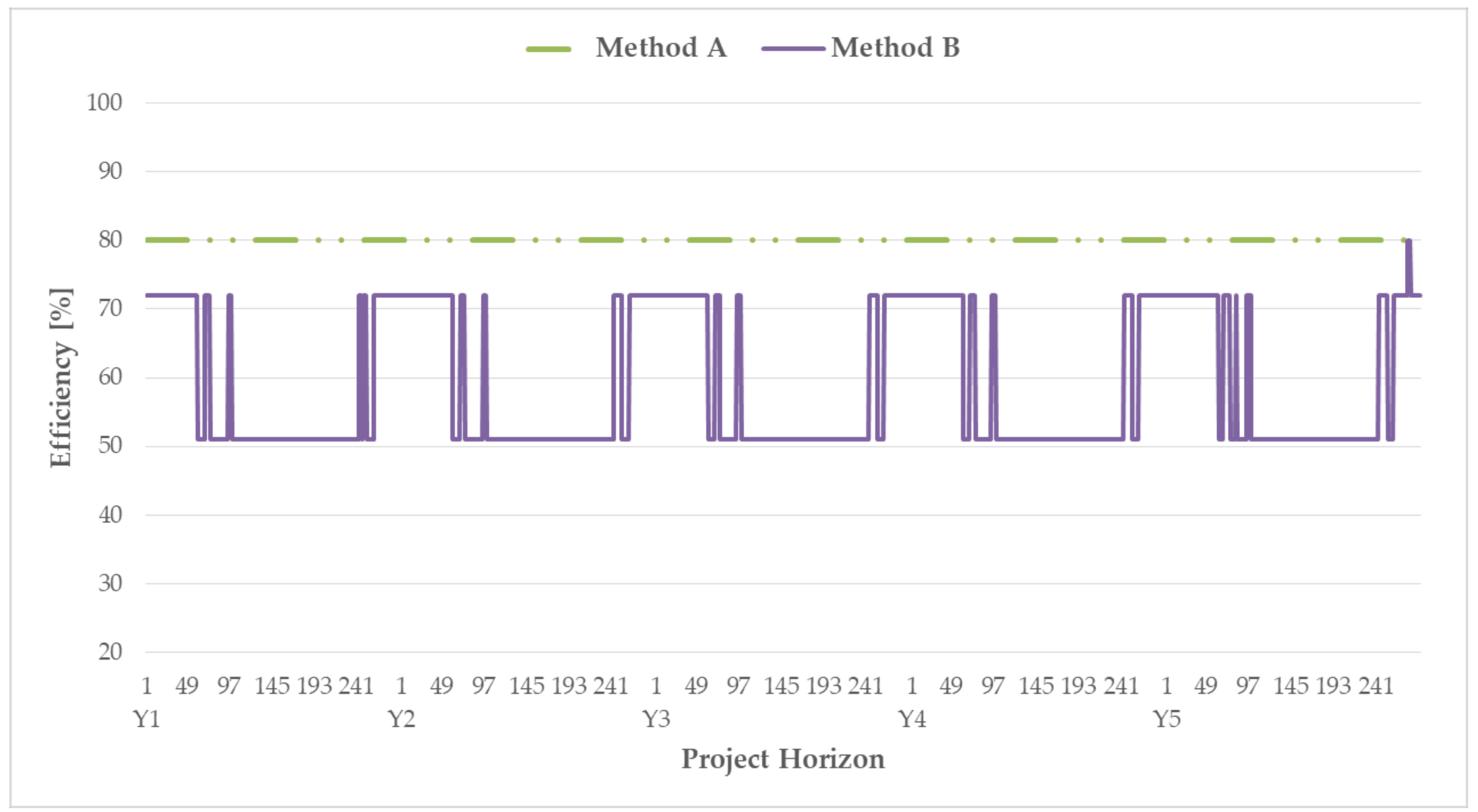
  • To validate the proposed method, the conventional optimization model using constant heat-to-power ratio and generation efficiency of the CHP resource is compared to the proposed optimization model in a case study.
The rest of this paper is organized as follows. Section 2 describes generation expansion planning model for integrated energy systems along with its objective function and constraints. We then introduce the optimization model considering the feasible operation region and generation efficiency function of the CHP resource in Section 3. A comparison between the conventional and the proposed expansion planning is detailed through a case study in Section 4 and we draw conclusions in Section 5.

2. Generation Expansion Planning Model for Integrated Energy Systems

This section provides an overview of the integrated energy system and optimization model for expansion planning using MILP.

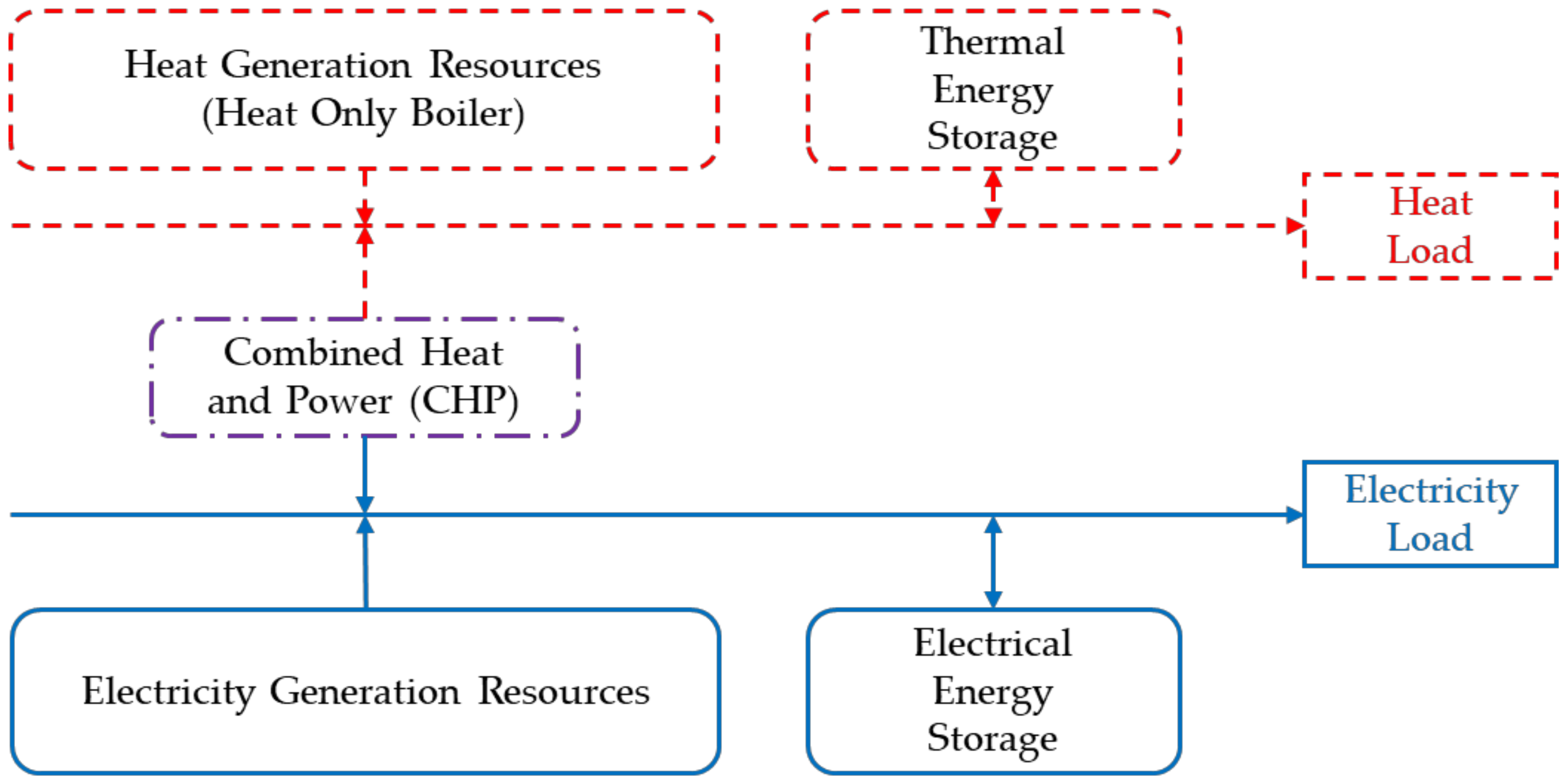
2.1. Integrated Energy System Model

We use an integrated energy system model from a previous study [28]. The system is assumed to be self-sufficient and its model is depicted in Figure 1. In the model, the CHP resource as well as heat and electricity generation resources are depicted with unidirectional units. In contrast, thermal and electrical energy storage are configured as bidirectional units given their ability for charging and discharging.

2.2. Objective Function

The proposed generation expansion planning model for an integrated energy system aims to minimize the sum of the annualized costs, including initial investment and operation costs of the CHP resource as well as heat and electrical energy resources over planning horizon N Y . Hence, the objective function is defined as
Minimize   y = 1 N Y ( ( 1 + γ d ) y ( COS T e y + COS T h y + COS T C H P y ) ) ,
considering costs
COS T e y = i = 1 N E R ( ( C R F e i C C e i + F O M C e i ) c = 1 N C ( C e i , c ν e i , c , y ) + ( F C e i + V O M C e i ) t = 1 N T F e i , t , y ) ,
COS T h y = j = 1 N H R ( ( C R F h j C C h j + F O M C h j ) c = 1 N C ( C h j , c ν h j , c , y ) + ( F C h j + V O M C h j ) t = 1 N T F h j , t , y ) ,
COS T C H P y = c h = 1 N C H P ( ( C R F C H P c h C C C H P c h + F O M C C H P c h ) c = 1 N C ( C C H P c h , c ν C H P c h , c , y ) ) + c h = 1 N C H P ( ( F C C H P c h + V O M C C H P c h ) t = 1 N T F C H P c h , t , y ) y ,
where
C R F e i = γ d ( 1 + γ d ) L T e i ( 1 + γ d ) L T e i 1 ,   C R F h j = γ d ( 1 + γ d ) L T h j ( 1 + γ d ) L T h j 1 ,   C R F C H P c h = γ d ( 1 + γ d ) L T C H P c h ( 1 + γ d ) L T C H P c h 1 i , j , c h ,
are the capital recovery factors from electrical and heat energy resources and CHP resources. C O S T e y , C O S T h y and C O S T CHP y are the respective total costs by energy resources for planning year y . Each cost comprises the annual fixed costs (including capital costs and fixed operation and maintenance costs related to the resource capacity) and the annual variable costs (including fuel costs and variable operation and maintenance costs related to fuel consumption). Equations (2)–(4) express the respective sum of annualized fixed and variable costs of resources. The annual fixed costs per unit capacity consist of capital recovery factors ( C R F e i , C R F h j and C R F CHP c h ), overnight capital costs ( C C e i , C C h j and C C CHP c h ) and fixed operation and maintenance costs ( F O M C e i , F O M C h j and F O M C CHP c h ). The fixed costs are determined by the capacity of a candidate unit ( C e i , c , C h j , c and C CHP c h , c ) of being selected with corresponding decision variable ( v e i , c , y , v h j , c , y and v CHP c h , c , y ). Likewise, the annual variable costs per unit consist of fuel costs ( F C e i , F C h j and F C CHP c h ) and variable operation and maintenance costs ( V O M C e i , V O M C h j and V O M C CHP c h ). The variable costs are determined by the fuel consumption per hour ( F e i , t , y , F h j , t , y and F CHP c h , t , y ).

2.3. Constraints for Heat and Electrical Energy Resources

The fuel consumption of heat and electrical energy resources depends on their generation efficiency and power output:
F e i , t , y = P e i , t , y η e i ,   F h j , t , y = P h j , t , y η h j j ,   t ,   y .
The output of heat and electricity is limited by the capacity of the selected resource and its minimum and maximum generation levels are given by
γ e , min i c = 1 N C ( C e i , c ν e i , c , y ) P e i , t , y γ e , max i c = 1 N C ( C e i , c ν e i , c , y ) j ,   t ,   y , γ h , min j c = 1 N C ( C h j , c ν h j , c , y ) P h j , t , y γ h , max j c = 1 N C ( C h j , c ν h j , c , y ) j ,   t ,   y .

2.4. Constraints for Electrical and Thermal Energy Storage Resources

The energy storage resources can charge and discharge energy within their state of charge (SOC) limits. Hence, stored energy is limited by the minimum and maximum SOC levels:
S O C E E S , min i = 1 N E R ( ρ E E S i c = 1 N C ( C e i , c v e i , c , y ) ) E E E S t , y S O C E E S , max i = 1 N E R ( ρ E E S i c = 1 N C ( C e i , c v e i , c , y ) ) , S O C T E S , min j = 1 N H R ( ρ T E S j c = 1 N C ( C h j , c v h j , c , y ) ) E T E S t , y S O C T E S , max j = 1 N H R ( ρ T E S j c = 1 N C ( C h j , c v h j , c , y ) ) .
The amount of stored energy decreases or increases during discharging or charging, respectively, except for the initially stored energy, as described by
E E E S t , y = { E E E S 0 , y , if t = 1 E E E S t 1 , y i = 1 N E R ( ρ E E S i P e i , t 1 , y / η E E S , e f f ) + P c h , e t 1 , y η E E S , e f f , otherwise t ,   y , E T E S t , y = { E T E S 0 , y , if t = 1 E T E S t 1 , y j = 1 N H R ( ρ T E S j P h j , t 1 , y / η T E S , e f f ) + P c h , h t 1 , y η T E S , e f f , otherwise t ,   y .
The amount of discharging or charging energy is limited by the capacity of energy storage resources, which can only operate in one mode at a given time. These storage characteristics can be described as
i = 1 N E R ( ρ E E S i P e i , t , y ) γ E E S , d c h ( 1 v c h , e t , y ) i = 1 N E R ( ρ E E S i c = 1 N C ( C e i , c v e i , c , y ) ) t ,   y , j = 1 N H R ( ρ T E S j P h j , t , y ) γ T E S , d c h ( 1 v c h , h t , y ) j = 1 N H R ( ρ T E S j c = 1 N C ( C h j , c v h j , c , y ) ) t ,   y ,
P c h , e t , y γ E E S , c h v c h , e t , y i = 1 N E R ( ρ E E S i c = 1 N C ( C e i , c v e i , c , y ) ) t ,   y , P c h , h t , y γ T E S , c h v c h , h t , y j = 1 N H R ( ρ T E S j c = 1 N C ( C h j , c v h j , c , y ) ) t ,   y ,
v c h , e t , y 1   t ,   y , v c h , h t , y 1 t   ,   y .
Note that linearization is required for MILP, because Equations (10) and (11) are nonlinear constraints. This linearization process is detailed in Appendix A.

2.5. Energy Balance Constraints

The heat and electrical load and charging load are supplied every hour by all energy resources, as described by
i = 1 N E R P e i , t , y + c h = 1 N C H P P C H P , e c h , t , y = l d e t , y + P c h , e t , y   t ,   y , j = 1 N H R P h j , t , y + c h = 1 N C H P P C H P , h c h , t , y = l d h t , y + P c h , h t , y   t ,   y .

3. Feasible Operation Region and Generation Efficiency of CHP Resource

This section describes the feasible operation region and the generation efficiency functions of the CHP resource. In addition, these are modeled with optimization constraints for using MILP.

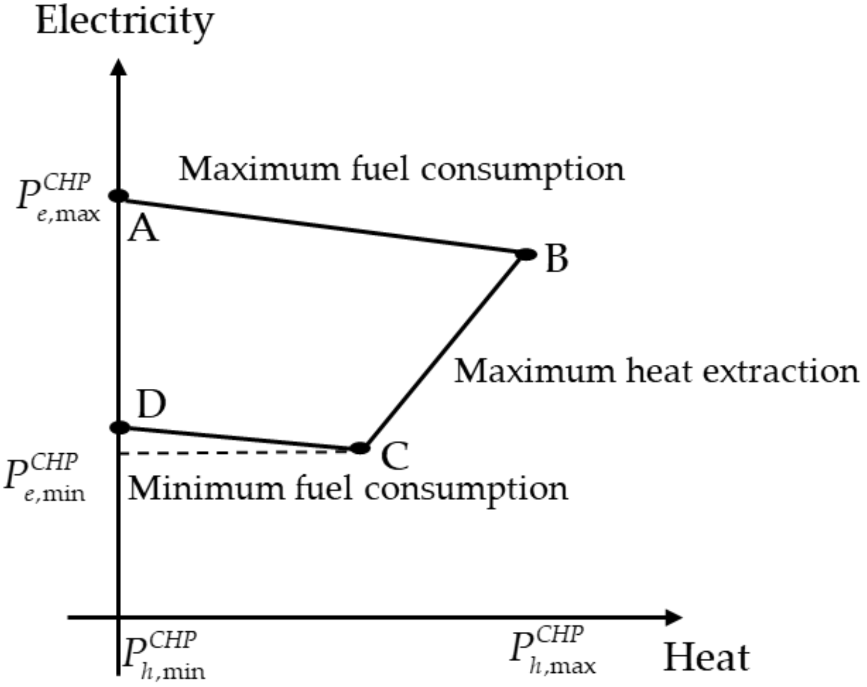
3.1. Feasible Operation Region for CHP Resource

Heat and electricity generated from the CHP resource depend on the feasible operation region [29,30], which is depicted by polyhedrons as shown in Figure 2.
The polyhedral region consists of four CHP operating points. The points A and B represent the maximum electricity and heat generation, respectively and their joining segment defines the maximum fuel consumption. The points C and D represent the minimum electricity generation and heat generation, respectively and their joining segment defines the minimum fuel consumption. The segments between the points A and D and between the points B and C define the operation range of only electricity generation and maximum heat extraction, respectively.
Heat and electricity generation belong to the region within the abovementioned segments and are defined by Equations (14)–(17). The following condition must be satisfied for the CHP resource to generate heat and electrical energy when the resource is committed:
0 P C H P , e c h , t , y P C H P , e c h , A v C H P c h , y   t ,   y , 0 P C H P , h c h , t , y P C H P , h c h , B v C H P c h , y   t ,   y ,
where P CHP , e c h , A and P CHP , h c h , B are the maximum operating points of electricity and heat generation, respectively. The operating condition within the segment of maximum fuel consumption is defined as
P C H P , e c h , t , y P C H P , e c h , A ( P C H P , e c h , A P C H P , e c h , B ) ( P C H P , h c h , A P C H P , h c h , B ) ( P C H P , h c h , t , y P C H P , h c h , A ) 0   t ,   y .
Other operating conditions within the segments of maximum heat extraction and minimum fuel consumption are respectively defined as
P C H P , e c h , t , y P C H P , e c h , B ( P C H P , e c h , B P C H P , e c h , C ) ( P C H P , h c h , B P C H P , h c h , C ) ( P C H P , h c h , t , y P C H P , h c h , B ) ( 1 v C H P c h , y ) Z   t ,   y ,
P C H P , e c h , t , y P C H P , e c h , C ( P C H P , e c h , C P C H P , e c h , D ) ( P C H P , h c h , C P C H P , h c h , D ) ( P C H P , h c h , t , y P C H P , h c h , D ) ( 1 v C H P c h , y ) Z   t ,   y ,
where P CHP , e c h , C and P CHP , h c h , D are the minimum operating points of electricity and heat generation, respectively and Z is a sufficiently large constant close to positive infinity. These equations of the operating segments are greater than negative infinity or zero, ( ( 1 v CHP c h , y ) Z ). These inequalities without negative infinity are not satisfied if the CHP resource is not committed, because these regions do not contain a zero operating point of electricity generation.

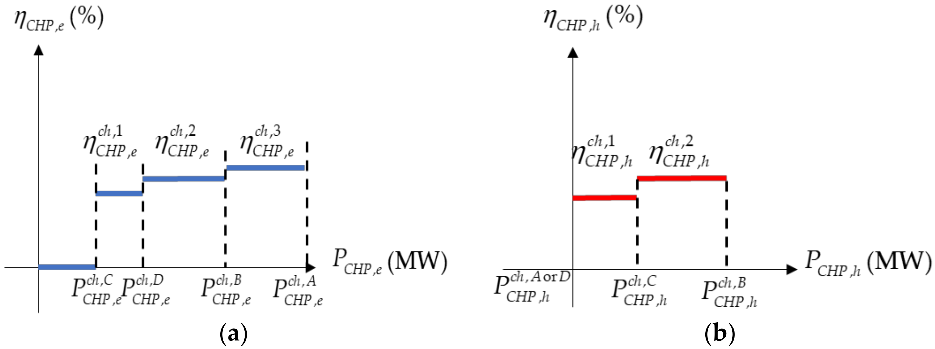
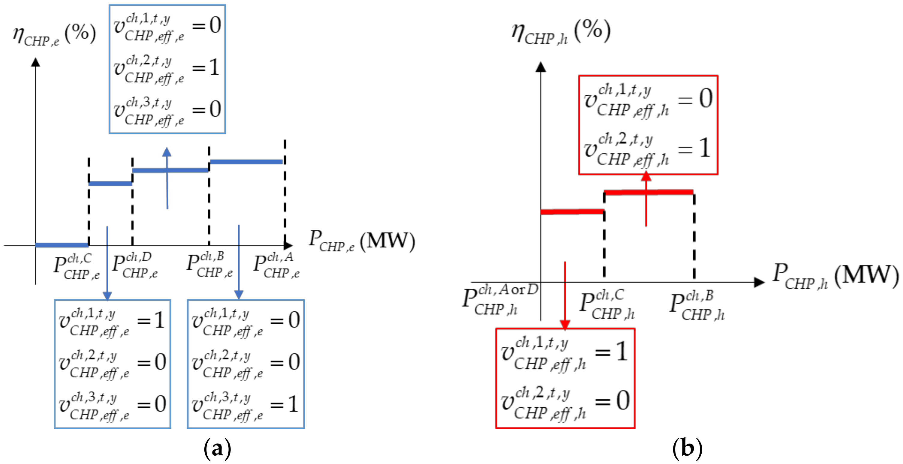
3.2. Efficiency Functions of CHP Resource

We assume that the generation efficiency of the CHP resource is varied with the generated heat or electricity over the feasible operation region based on the function of loading level of the CHP resource [31]. The efficiency functions for the CHP resource are also assumed to be modeled by discrete functions, which are required for MILP and illustrate the relationship between generation efficiency and output, as shown in Figure 3.
The efficiency functions for the CHP resource are assumed to be modeled by the mean value of the generation efficiency over segments on the feasible operation region. Therefore, the number of boundary segments of these functions are 3 and 2, respectively.
Variables for selecting efficiency segments are determined considering the generation efficiency varying with the generation of the CHP resource as follows:
ν C H P , e f f , e c h , b e , t , y { 0 , 1 } c h ,   b e ,   t ,   y , ν C H P , e f f , h c h , b h , t , y { 0 , 1 } c h ,   b h ,   t ,   y ,
where be and bh are indices of the boundary segments of electricity and heat generation efficiency function, respectively. Each of these variables is equal to 1 if the corresponding CHP resource generates electrical energy determined in the specific efficiency segment and it is equal to 0 otherwise. Examples of segment selection with these variables are illustrated in Figure 4.
The generation output of the CHP resource should be defined in the boundary segments of the efficiency function to also guarantee that the output is within the feasible operation region. The heat and electricity generation is defined as
{ P C H P , e c h , t , y ( 1 v C H P , e f f , e c h , b e , t , y ) Z + v C H P , e f f , e c h , b e , t , y P C H P , e c h , b e + 1 P C H P , e c h , t , y ( 1 v C H P , e f f , e c h , b e , t , y ) Z + v C H P , e f f , e c h , b e , t , y P C H P , e c h , b e c h ,   b e ,   t ,   y , { P C H P , h c h , t , y ( 1 v C H P , e f f , h c h , b h , t , y ) Z + v C H P , e f f , h c h , b h , t , y P C H P , h c h , b h + 1 P C H P , h c h , t , y ( 1 v C H P , e f f , h c h , b h , t , y ) Z + v C H P , e f f , h c h , b h , t , y P C H P , h c h , b h c h ,   b h ,   t ,   y .
For example, if the electricity generation of the committed CHP resource is within the first boundary segment of Figure 4a, the first boundary segment selecting variable is 1. Then, according to Equation (19), the electricity generation is bigger than P C H P , e c h , C and lower than P C H P , e c h , D . In other boundary segments, the electricity generation is bigger than negative infinity and lower than positive infinity since other selecting variables are 0. The additional condition is required since the boundary segment can only be selected once or not at all:
b e = 1 N B E v C H P , e f f , e c h , b e , t , y = v C H P c h , y   c h ,   t ,   y , b h = 1 N B H v C H P , e f f , h c h , b h , t , y = v C H P c h , y   c h ,   t ,   y .
With these conditions, the variables for selecting boundary segments can be decided according to the generation output.
Finally, the fuel consumption of the CHP resource is defined as the generation output and efficiency determined by the abovementioned procedures:
F C H P , e c h , t , y = b e = 1 N B E ( P C H P , e c h , t , y η C H P , e c h , b e v C H P , e f f , e c h , b e , t , y ) c h ,   t ,   y , F C H P , h c h , t , y = b h = 1 N B H ( P C H P , h c h , t , y η C H P , h c h , b h v C H P , e f f , h c h , b h , t , y ) c h ,   t ,   y .
Linearization is required because the constraints on fuel consumption of CHP resources correspond to the product of variables. This linearization process is detailed in Appendix B.

4. Case Study and Discussion

We evaluated the effectiveness of the proposed method by comparing with the planning results using conventional generation expansion planning model.

4.1. Simulation Setup

We applied the proposed optimization model to a comprehensive integrated energy system with peak electricity demand of 1213.2 MW and peak heat demand of 956.8 MW [32,33]. The key parameters of the optimization model are listed in Table 1.
The planning horizon of 5 years considers 288 h (24 h × 12 months) per year instead of the total 8760 h to reduce the computational burden. The annual interest rate and demand growth rate are considered according to [34]. We considered the profiles of peak and mean load per month to generate the 288-h load profiles. The complete 8760-h load profiles were categorized by hour and month. For generating the peak load profiles, single-day load profiles containing the peak load per month were extracted from the 8760-h load profiles. To generate the mean load profiles, we calculated the average load every hour per month. Then, we collected the peak and mean load profiles considering the demand growth rate for 5 years to obtain the profiles shown in Figure 5.
The cost and size data of the energy resources are listed in Appendix C Table A1. With the cost data, the operation data including the efficiency and operating point data are required. We used the operation data from the actual CHP resource technology listed in Table 2 [29,35,36]. The operating points in this table were designed based on the feasible operation region shown in Figure 2. In addition, operating points B and C of heat generation are equal to 0.92 times the electricity generation at operating points B and C, respectively, because the assumed CHP was designed with an average heat-to-power ratio of 0.92.
Apart from CHP, other energy resources were assumed to have a constant generation efficiency. We also used the minimum and maximum generation limits of electrical and heat energy resources listed in Table 3 and the operation conditions for energy storage listed in Table 4.

4.2. Simulation Results

We solved the proposed MILP optimization problem using intlinprog with Gurobi optimization in MATLAB (Mathworks, Inc., Natick, MA, USA). The dual simplex algorithm terminated after reaching a 0.1% duality gap. We compared the planning results of the proposed method and those of conventional method using constant heat-to-power ratio and generation efficiency of the CHP resource for supplying the peak and mean loads from the profiles shown in Figure 5. The heat-to-power ratio was assumed to be 0.92 and the generation efficiency was assumed to be 80% from the sum of the first boundary segments of electrical and heat generation efficiency in Table 2. The maximum electricity and heat generation of the CHP resource were assumed to be point A of electricity and heat generation in Table 2. We classified optimization models applied to expansion planning as detailed in Table 5.

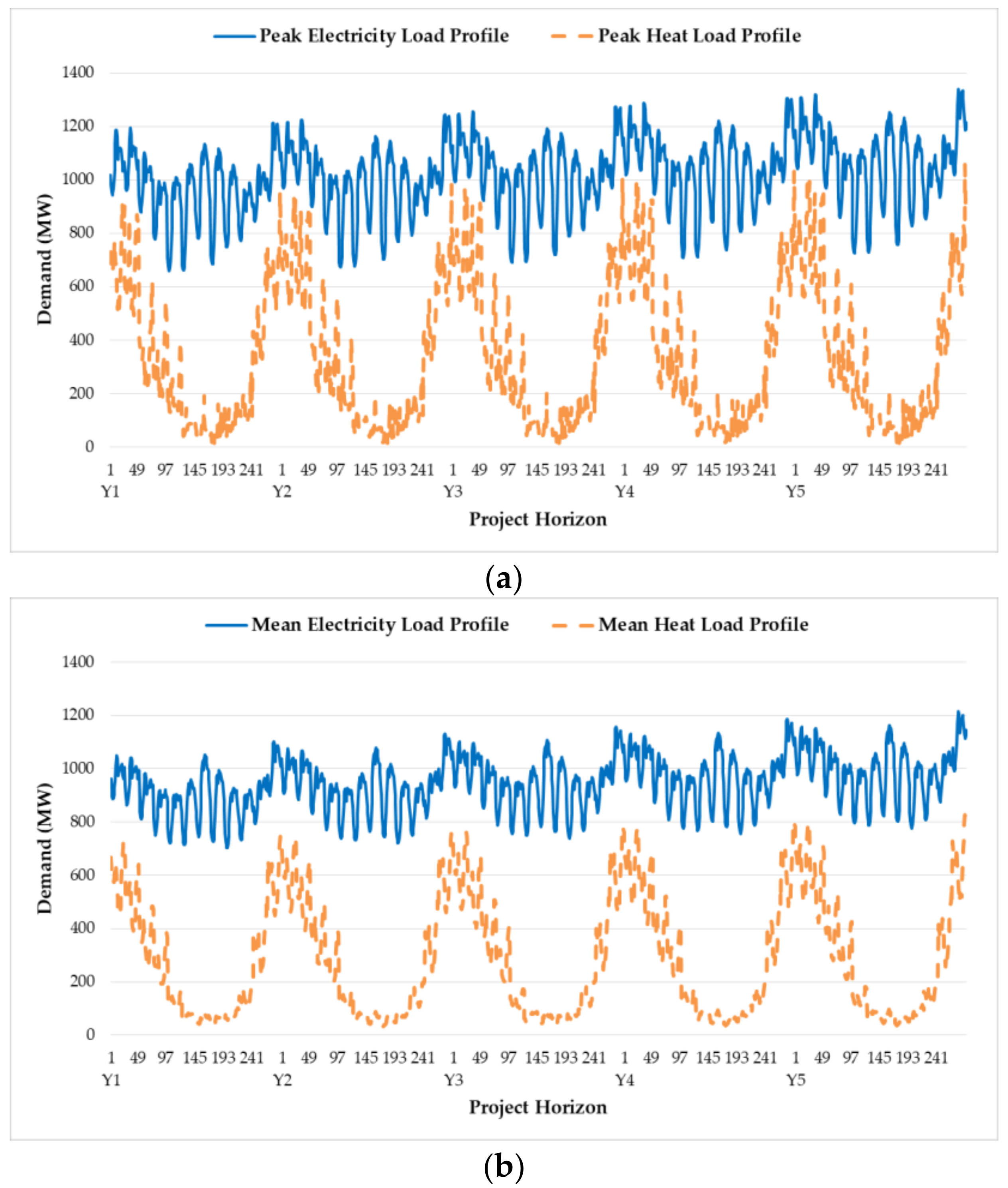
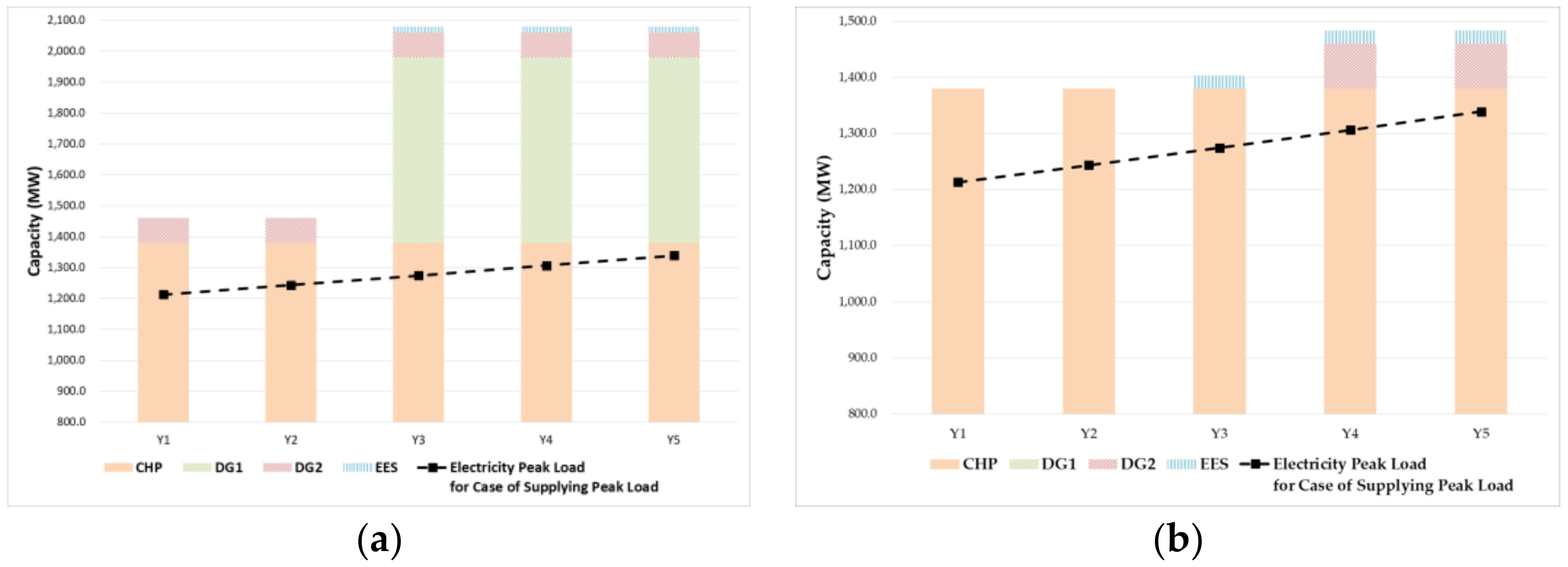
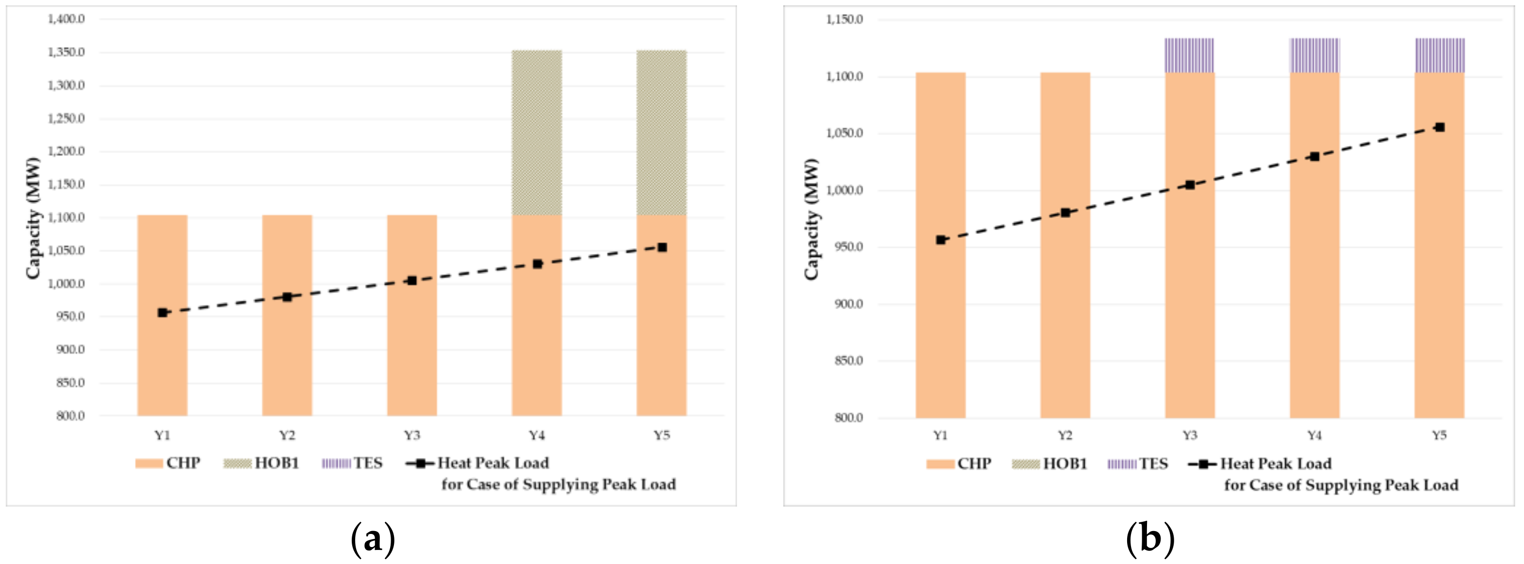
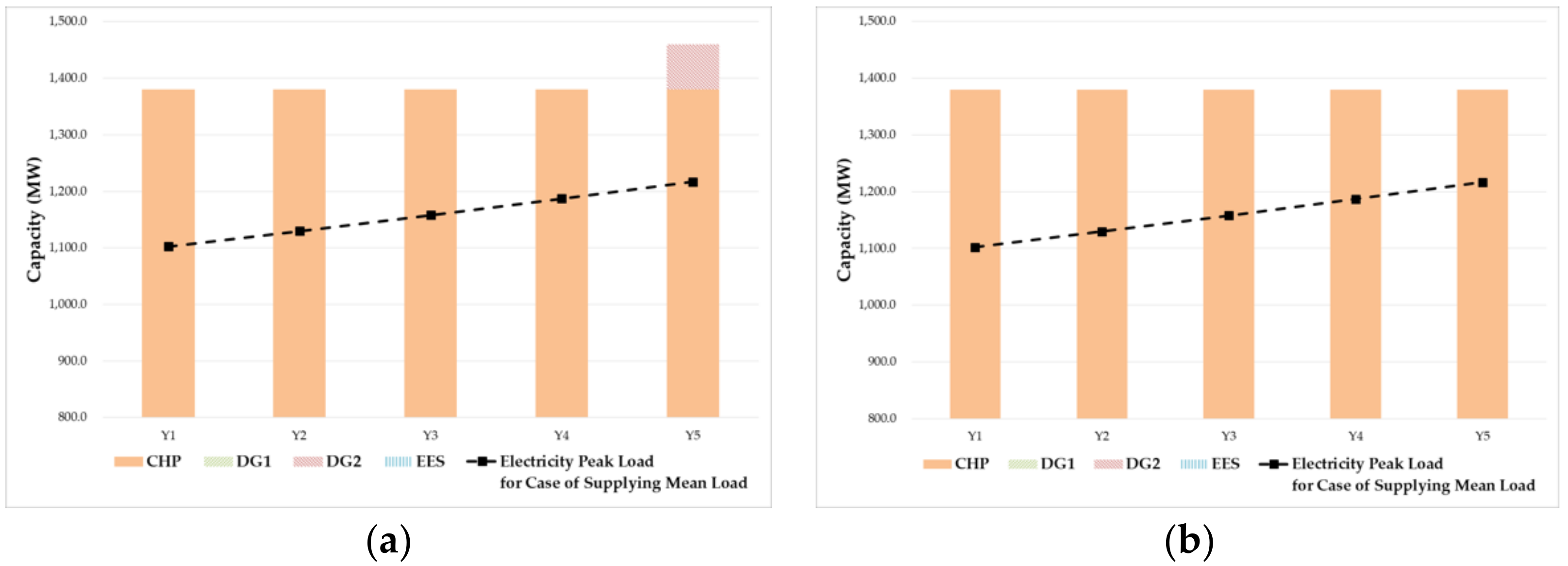
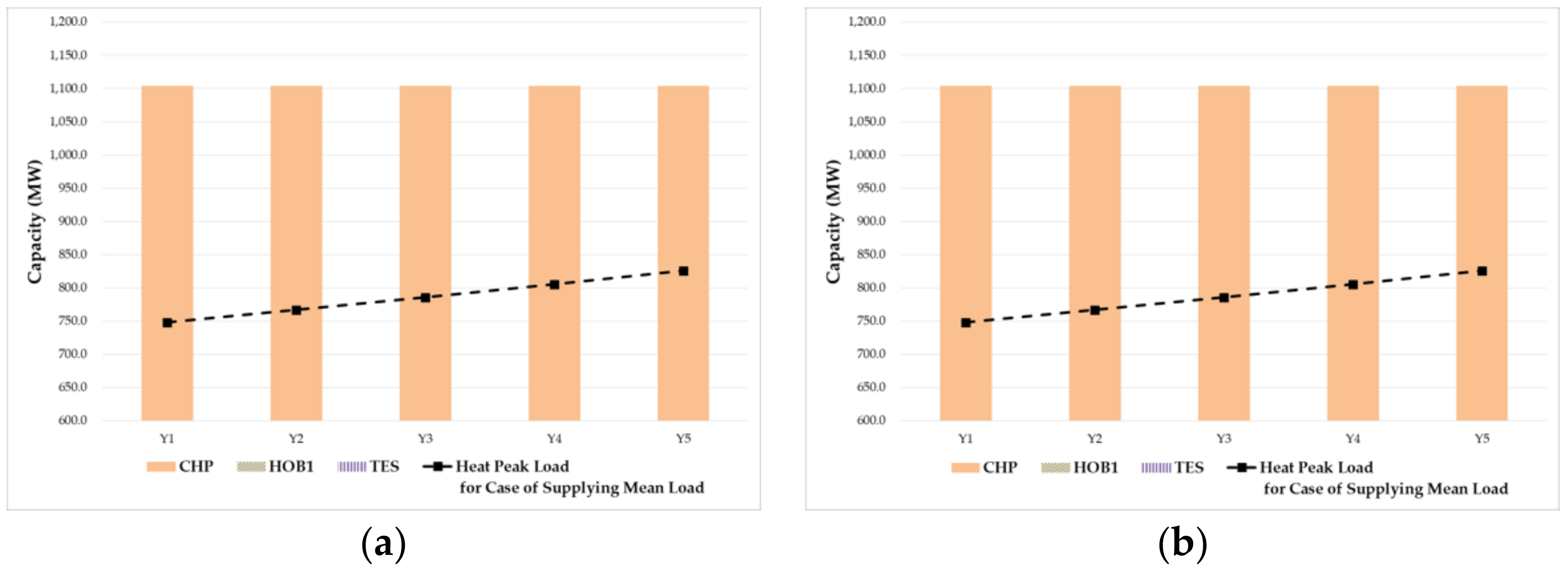
4.2.1. Peak Load Supply

The cost results by optimization models for peak load supply are listed in Table 6. In addition, the percent variation from the costs of model A to those of model B are listed in the table. Most of the costs including the total cost obtained from model A were higher than those obtained from model B. Although the costs of the CHP resource in models A and B were very similar, those of electrical and heat energy resources in model A are at least 78% higher than those in model B. Consequently, the cost results suggest the number of built electrical and heat resources in model A is greater than that in model B.
The difference of the generation expansion planning results using models A and B is depicted in Figure 6 and Figure 7. Figure 6 shows the planning schedules for supplying peak electricity load, whereas Figure 7 shows those for supplying peak heat load. The total capacity of electrical energy resources in the planning obtained from model A was much larger than that from model B as shown in Figure 6a, because electricity generation of the CHP resource in model A was limited by the constant heat-to-power ratio. In model A, even a high electricity demand retrieved a low amount of electricity generation of the CHP resource when heat generation was low. On the other hand, the total capacity using model B did not exceed 15% of the peak load per year as shown in Figure 6b. The electricity generation of the CHP resource in model B was not relatively limited by the heat-to-power ratio as in model A, because this resource can flexibly generate heat and electricity on the feasible operation region. Therefore, the difference between planning schedules using models A and B was considerable, especially during year Y3, where all the electricity generation resources were installed in model A for supplying the electricity peak load, whereas electricity generation resource DG1 was not installed in model B. This difference was notably reflected in the costs obtained from the models.
The planning schedules for supplying heat peak load were very similar to those for supplying electricity peak load. Heat generation of the CHP resource can supply enough heat load until planning year Y2, as the heat peak load was much below its capacity. In model B, energy storage resource TES was installed on planning year Y3 for utilizing surplus heat, whereas in model A, boiler HOB1 was installed from planning year Y4 for supplying heat load through the CHP resource.
The total generation efficiency profiles of the CHP resource by the optimization models for supplying peak load are depicted in Figure 8. The profile of model A corresponds to the horizontal line, whereas the profile of model B varies along the project horizon. Overall, the total generation efficiency of the CHP resource using model A was higher than that using model B. Hence, the total variable cost of the CHP resource using model B was mostly higher than that using model A. Using model B, the total generation efficiency can be inferred from periods in the project horizon. For instance, the total generation efficiency in the period from 1 to 48 (i.e., from January to February) was mostly the highest because the CHP resource should supply a large heat demand during winter. In contrast, the total generation efficiency in the period from 144 to 240 (i.e., from June to October) was mostly the lowest because heat demand was low. From planning year Y3, the total generation efficiency reached the lowest value during summer because the operation of energy storage resource TES substituted the small amount of heat generation required from the CHP resource.

4.2.2. Mean Load Supply
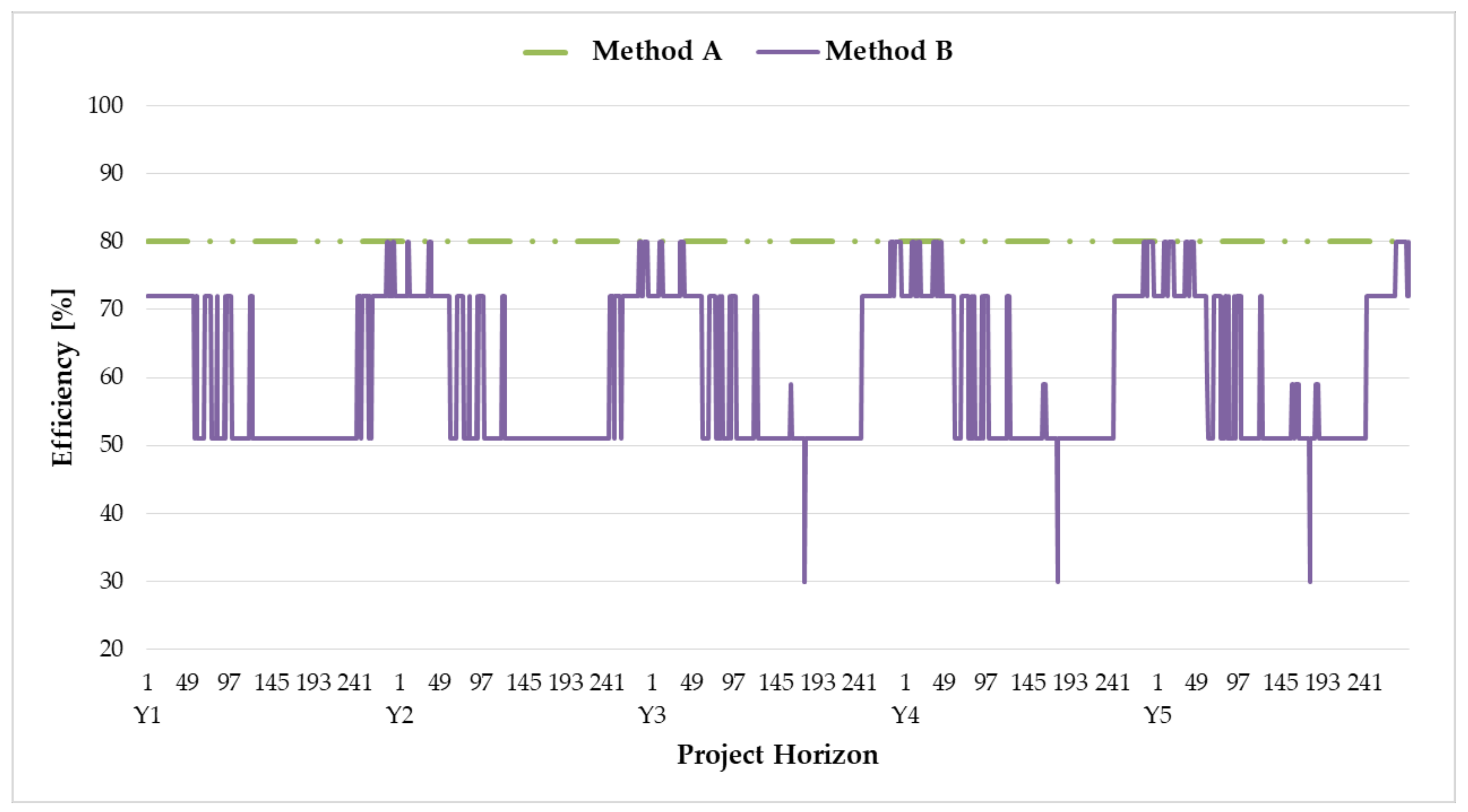
The cost results by optimization models for mean load supply are listed in Table 7. Similar to the case of supplying peak load, the costs including the total cost obtained from model A were higher than those obtained from model B. Unlike the case of supplying peak load, the percent variance of the total cost between models A and B was small given the smaller electricity and heat demand in the mean load profile than in the peak load profile. Although the percent variance of costs of CHP resources and heat energy resources was small or zero, that of electrical energy resources was 100%. Overall, most of the heat and electricity mean load can be supplied by the CHP resource.
The difference of the generation expansion planning results using models A and B is depicted in Figure 9 and Figure 10. Unlike the planning schedules in Figure 6, the CHP resource can cover the electricity load except for planning year Y5 using model A, as shown in Figure 9. Electrical energy resource DG2 should be installed to compensate the electricity shortage due to the constant heat-to-power ratio of the CHP resource when using model A. The expansion planning results for heat energy resources were equal regardless of the model, as shown in Figure 10. Only the CHP resource supplied the heat load without any additional resources.
The total generation efficiency profiles of the CHP resource by the optimization models for mean load supply are depicted in Figure 11. Like in Figure 8, the total generation efficiency of the CHP resource using model A was higher than that using model B but for mean load, the profile using model B was more regular than that profile of supplying peak load, being between 50% and 80%. The profile using model B did not fluctuate greatly because CHP supplied most of the electricity and heat load.

4.3. Discussions

The proposed optimization model could be utilized for either planning or managing energy resources in the integrated energy systems. Unlike conventional expansion planning models using constant heat-to-power ratio and generation efficiency, the proposed model could provide a cost-effective expansion plan as verified in the results. Moreover, the obtained results would be utilized as indicators for seasonal changes in operation of CHP resources. Although the generation efficiency of CHP resources should be thoroughly considered in energy expansion planning, most of the available studies and policies have overlooked details about the generation efficiency regarding seasonal changes. Therefore, the proposed model can provide more reliable scenarios for the integrated energy system planning under conditions that resemble the actual operation of CHP resources.

5. Conclusions

We propose a method of generation expansion planning for an integrated energy system. Although the objective function and constraints of the conventional heat and electrical energy resources were similar to those of other methods, we also considered the feasible operation region and the generation efficiency of the CHP resource. To apply these operation characteristics into the generation expansion planning problem modeled as a MILP, we linearized the cost function and constraints of the CHP resource. We compared 5-year planning results between the conventional optimization model applying constant heat-to-power ratio and generation efficiency of the CHP resource and the proposed optimization model. The models considered supplying peak and mean loads of the integrated energy system, retrieving remarkable differences among the resulting plans. In fact, heat and electrical energy resources were installed appropriately according to variations of loads using the proposed method. Although the overall generation efficiency of the CHP resource using the proposed model was lower than that using the conventional one, the total costs of the proposed model were lower than those of the conventional one. We expect that the proposed method will allow planners and operators of integrated energy systems to design and optimize their systems under conditions very similar to the actual operation of the CHP resource.

Author Contributions

All the authors contributed to this work. W.K. designed the study, performed the analysis and wrote the first draft of the paper. J.K. contributed to the conceptual approach and thoroughly revised the paper.

Acknowledgments

This work was supported by the Korea Institute of Energy Technology Evaluation and Planning (KETEP) and the Ministry of Trade, Industry & Energy (MOTIE) of the Republic of Korea (No. 20181210301380).

Conflicts of Interest

The authors declare no conflict of interest.

Nomenclature

Indices
y Project year index, from [ 1 : N Y ] .
i Electrical energy resource index, from [ 1 : N E R ] .
j Heat energy resource index, from [ 1 : N H R ] .
c h Combined heat and power resource index, from [ 1 : N C H P ] .
c Candidate unit index, from [ 1 : N C ] .
b e Section index of electricity generation efficiency for CHP resource, from [ 1 : N B E ] .
b h Section index of heat generation efficiency for CHP resource, from [ 1 : N B H ] .
Variables of electrical energy resources
P e i , t , y Generation output of the electrical energy resource, i , for hour, t , is allocated in project year, y (MW).
F e i , t , y Fuel usage of the electrical energy resource, i , for hour, t , is allocated in project year, y (MWh).
E E E S t , y Stored energy of EES for hour, t , in project year, y (MWh).
P c h , e t , y Charging power of EES for hour, t , in project year, y (MW).
φ c h , e t , y Variable for linearizing charging power constraints.
φ d c h , e t , y Variable for linearizing discharging power constraints.
v e i , c , y Status of candidate generating unit, c , of electrical energy resource, i , in project year, y .
v c h , e t , y Binary variable for selecting charging or discharging operation of the electrical energy storage.
Variables of heat energy resources
P h j , t , y Generation output of the heat energy resource, j , for hour, t , is allocated in project year, y (MW).
F h j , t , y Fuel usage of the heat energy resource, j , for hour, t , is allocated in project year, y (MWh).
E T E S t , y Stored energy of TES for hour, t , in project year, y (MWh).
P c h , h t , y Charging power of TES for hour, t , in project year, y (MW).
φ c h , h t , y Variable for linearizing charging power constraints.
φ d c h , h t , y Variable for linearizing discharging power constraints.
v h j , c , y Status of candidate generating unit, c , of heat energy resource, j , in project year, y .
v c h , h t , y Binary variable for selecting charging or discharging operation of the heat energy storage.
Variables of CHP resources
P C H P , e c h , t , y Electricity generation output of CHP resource, c h , for hour, t , is allocated in project year, y (MW).
P C H P , h c h , t , y Heat generation output of CHP resource, c h , for hour, t , is allocated in project year, y (MW).
F C H P , e c h , t , y Fuel usage of electricity output of CHP resource, c h , for hour,   t , is allocated in project year, y (MWh).
F C H P , h c h , t , y Fuel usage of heat output of CHP resource, c h , for hour,   t , is allocated in project year, y (MWh).
η C H P c h , t , y Overall generation efficiency of CHP resource, c h , for hour,   t , is allocated in project year, y (MWh).
φ c h p , e c h , b e , t , y Variable for linearizing constraints of selecting efficiency section of electricity generation of CHP resource.
φ c h p , h c h , b h , t , y Variable for linearizing constraints of selecting efficiency section of heat generation of CHP resource.
v C H P c h , y Status of CHP resource, c h , in project year, y .
v C H P , e f f , e c h , b e , t , y Binary variable for selecting efficiency segment of electricity generation of CHP resource.
v C H P , e f f , h c h , b h , t , y Binary variable for selecting efficiency segment of heat generation of CHP resource.
Parameters
C e i , c Capacity of candidate generating unit, c , of electrical energy resource, i .
C h j , c Capacity of candidate generating unit, c , of heat energy resource, j .
C C e i Capital cost of electrical energy resource, i .
C C h j Capital cost of heat energy resource, j .
C C C H P c h Capital cost of CHP resource, c h .
F O M C e i Fixed operation and maintenance cost of electrical energy resource, i .
F O M C h j Fixed operation and maintenance cost of heat energy resource, j .
F O M C C H P c h Fixed operation and maintenance cost of CHP resource, c h .
F C e i Fuel cost of electrical energy resource, i .
F C e j Fuel cost of heat energy resource, j .
F C C H P c h Fuel cost of CHP resource, c h .
V O M C e i Variable operation and maintenance cost of electrical energy resource, i .
V O M C h j Variable operation and maintenance cost of heat energy resource, j .
V O M C C H P c h Variable operation and maintenance cost of CHP resource, c h .
L T e i Lifetime of electrical energy resource, i .
L T h j Lifetime of heat energy resource, j .
L T C H P c h Lifetime of CHP resource, c h .
P C H P , e c h , o p Operating point of electricity generation, o p , of CHP resource, c h .
P C H P , h c h , o p Operating point of heat generation, o p , of CHP resource, c h .
η C H P , e c h , b e Electricity generation efficiency of section, b e , of CHP resource, c h .
η C H P , h c h , b h Heat generation efficiency of section, b h , of CHP resource, c h .
ρ E E S i Index of electrical energy storage in electrical energy resource, i .
ρ T E S j Index of thermal energy storage in heat energy resource, j .
γ e , m a x / γ e , m i n Maximum/Minimum generation limit of electrical energy resource.
γ h , m a x / γ h , m i n Maximum/Minimum generation limit of heat energy resource.
S O C E E S , m a x / S O C E E S , m i n Maximum/Minimum SOC limit of electrical energy storage
S O C T E S , m a x / S O C T E S , m i n Maximum/Minimum SOC limit of thermal energy storage
η E E S , d c h / η E E S , c h Discharging/Charging efficiency of electrical energy storage
η T E S , d c h / η T E S , c h Discharging/Charging efficiency of thermal energy storage
γ E E S , d c h / γ E E S , c h Cleared discharging/charging rate for electrical energy storage.
γ T E S , d c h / γ T E S , c h Cleared discharging/charging rate for thermal energy storage.
η E E S , e f f Turnaround efficiency for electrical energy storage
η T E S , e f f Turnaround efficiency for thermal energy storage
γ d Interest rate

Appendix A. Linearization of Nonlinear Constraints on Energy Storage

Equation (10) shows the nonlinear constraints during discharging of energy storage resources. The expressions on the right-hand side of these constraints can be divided into separate equations given by
{ φ d c h , e t , y ( 1 v c h , e t , y ) Z φ d c h , e t , y ( 1 v c h , e t , y ) Z t ,   y , { φ d c h , h t , y ( 1 v c h , h t , y ) Z φ d c h , h t , y ( 1 v c h , h t , y ) Z t ,   y ,
{ φ d c h , e t , y η E E S , d c h i = 1 N E R ( ρ E E S i c = 1 N C ( C e i , c v e i , c , y ) ) v c h , e t , y Z φ d c h , e t , y η E E S , d c h i = 1 N E R ( ρ E E S i c = 1 N C ( C e i , c v e i , c , y ) ) + v c h , e t , y Z t ,   y , { φ d c h , h t , y η T E S , d c h j = 1 N H R ( ρ T E S j c = 1 N C ( C h j , c v h j , c , y ) ) v c h , h t , y Z φ d c h , h t , y η T E S , d c h j = 1 N H R ( ρ T E S i c = 1 N C ( C h j , c v h j , c , y ) ) + v c h , h t , y Z t ,   y .
These separate equations compose four inequality constraints for variable φ dch , e t , y and φ dch , h t , y and Z . For example, if either v ch , e t , y or v ch , h t , y is equal to 0 when during discharges, φ dch , e t , y is the product of the discharging efficiency and the capacity of energy storage, as shown in Equation (A2). Otherwise, either φ dch , e t , y or φ dch , h t , y is equal to 0. Using the above inequality constraints and variables φ dch , e t , y and φ dch , h t , y , the nonlinear constraints can linearized as follows:
i = 1 N E R ( ρ E E S i P e i , t , y ) φ d c h , e t , y t ,   y , j = 1 N H R ( ρ T E S j P h j , t , y ) φ d c h , h t , y t ,   y .
Likewise, the nonlinear constraints in Equation (11) can also be linearized as follows:
{ φ c h , e t , y v c h , e t , y Z φ c h , e t , y v c h , e t , y Z t ,   y , { φ c h , h t , y v c h , h t , y × Z φ c h , h t , y v c h , h t , y × Z t ,   y ,
{ φ c h , e t , y η E E S , c h i = 1 N E R ( ρ E E S i c = 1 N C ( C e i , c v e i , c , y ) ) ( 1 v c h , e t , y ) Z φ c h , e t , y η E E S , c h i = 1 N E R ( ρ E E S i c = 1 N C ( C e i , c v e i , c , y ) ) + ( 1 + v c h , e t , y ) Z t ,   y , { φ c h , h t , y η T E S , c h j = 1 N H R ρ T E S j ( c = 1 N C ( C h j , c v h j , c , y ) ) ( 1 v c h , h t , y ) Z φ c h , h t , y η T E S , c h j = 1 N H R ( ρ T E S j c = 1 N C ( C h j , c v h j , c , y ) ) + ( 1 + v c h , h t , y ) Z t ,   y ,
P c h , e t , y φ c h , e t , y   t ,   y , P c h , h t , y φ c h , h t , y   t ,   y .
Although the number of constraints increases, linearization allows to apply MILP-based optimization considering the charging mode and status of the energy storage resources.

Appendix B. Linearization of the CHP Fuel Consumption

In Equation (21), fuel consumption of the CHP resource should be linearized to realize MILP-based optimization because it is composed of the product of the binary variable for generation efficiency segment and the electricity generation. The linearization proceeds as follows:
F C H P , e c h , t , y = b e = 1 N b e ( P C H P , e c h , t , y η C H P , e c h , b e v C H P , e f f , e c h , b e , t , y ) = b e = 1 N b e ( g C H P , e c h , b e , t , y v C H P , e f f , e c h , b e , t , y ) c h ,   t ,   y , F C H P , h c h , t , y = b h = 1 N b h ( P C H P , h c h , t , y η C H P , h c h , b h v C H P , e f f , h c h , b h , t , y ) = b h = 1 N b h ( g C H P , h c h , b h , t , y v C H P , e f f , h c h , b h , t , y ) c h ,   t ,   y ,
where either g CHP , e c h , b e , t , y or g CHP , h c h , b h , t , y equals to the product of the generation output and the reciprocal of the segment generation efficiency. For simplicity during linearization, the product of variables is substituted by either φ CHP , eff , e c h , b e , t , y or φ CHP , eff , h c h , b h , t , y as follows:
φ C H P , e f f , e c h , b e , t , y = g C H P , e f f , e c h , b e , t , y v C H P , e f f , e c h , b e , t , y c h ,   b e ,   t ,   y , φ C H P , e f f , h c h , b h , t , y = g C H P , e f f , h c h , b h , t , y v C H P , e f f , h c h , b h , t , y c h ,   b h ,   t ,   y .
These equations can be linearized based on linear inequality constraints as follows:
{ φ C H P , e f f , e c h , b e , t , y v C H P , e f f , e c h , b e , t , y Z φ C H P , e f f , e c h , b e , t , y v C H P , e f f , e c h , b e , t , y Z c h ,   b e ,   t ,   y , { φ C H P , e f f , h c h , b h , t , y v C H P , e f f , h c h , b h , t , y Z φ C H P , e f f , h c h , b h , t , y v C H P , e f f , h c h , b h , t , y Z c h ,   b h ,   t ,   y ,
{ φ C H P , e f f , e c h , b e , t , y g C H P , e f f , e c h , b e , t , y ( 1 v C H P , e f f , e c h , b e , t , y ) Z φ C H P , e f f , e c h , b e , t , y g C H P , e f f , e c h , b e , t , y + ( 1 v C H P , e f f , e c h , b e , t , y ) Z c h ,   b e ,   t ,   y , { φ C H P , e f f , h c h , b h , t , y g C H P , e f f , h c h , b h , t , y ( 1 v C H P , e f f , h c h , b h , t , y ) Z φ C H P , e f f , h c h , b h , t , y g C H P , e f f , h c h , b h , t , y + ( 1 v C H P , e f f , h c h , b h , t , y ) Z c h ,   b h ,   t ,   y .
Finally, the fuel consumption of CHP is composed of the sum of single variables:
F C H P , e c h , t , y = b e = 1 N b e φ C H P , e f f , e c h , b e , t , y c h ,   b e ,   t ,   y , F C H P , h c h , t , y = b h = 1 N b h φ C H P , e f f , h c h , b h , t , y c h ,   b h ,   t ,   y .

Appendix C. Cost Data

Table A1. Cost data of energy resources
Resource TypeUnit NameOvernight Capital Cost ($/MW)Fixed O&M Cost ($/MW)Fuel Cost ($/MWh)Variable O&M Cost ($/MWh)Life Span (Yr)Candidate Size (MW)
Fuel-based Power GeneratorDG1900,00015,00033.29256.120700, 600
DG2650,00015,000182.3152090, 80
Heat Only BoilerHOB1520,00015,000182.31520300, 250
CHPCHP1,150,000585022.772.75201200, 1000, 800
Electrical Energy StorageEES3,092,00010,000030724, 20
Thermal Energy StorageTES3,184,00012,000030730,20

References

  1. Mavromatidis, G.; Orehounig, K.; Carmeliet, J. A review of uncertainty characterisation approaches for the optimal design of distributed energy systems. Renew. Sustain. Energy Rev. 2018, 88, 258–277. [Google Scholar] [CrossRef]
  2. Koirala, B.; Chaves Ávila, J.; Gómez, T.; Hakvoort, R.; Herder, P. Local Alternative for Energy Supply: Performance Assessment of Integrated Community Energy Systems. Energies 2016, 9, 981–1004. [Google Scholar] [CrossRef]
  3. Ashouri, A.; Fux, S.S.; Benz, M.J.; Guzzella, L. Optimal design and operation of building services using mixed-integer linear programming techniques. Energy 2013, 59, 365–376. [Google Scholar] [CrossRef]
  4. Dominković, D.; Stark, G.; Hodge, B.-M.; Pedersen, A. Integrated Energy Planning with a High Share of Variable Renewable Energy Sources for a Caribbean Island. Energies 2018, 11, 2193–2207. [Google Scholar] [CrossRef]
  5. Amusat, O.O.; Shearing, P.R.; Fraga, E.S. Optimal integrated energy systems design incorporating variable renewable energy sources. Comput. Chem. Eng. 2016, 95, 21–37. [Google Scholar] [CrossRef] [Green Version]
  6. Amusat, O.O.; Shearing, P.R.; Fraga, E.S. Optimal design of hybrid energy systems incorporating stochastic renewable resources fluctuations. J. Energy Storage 2018, 15, 379–399. [Google Scholar] [CrossRef]
  7. Fioriti, D.; Giglioli, R.; Poli, D.; Lutzemberger, G.; Micangeli, A.; Del Citto, R.; Perez-Arriaga, I.; Duenas-Martinez, P. Stochastic sizing of isolated rural mini-grids, including effects of fuel procurement and operational strategies. Electr. Power Syst. Res. 2018, 160, 419–428. [Google Scholar] [CrossRef]
  8. Borelli, D.; Devia, F.; Lo Cascio, E.; Schenone, C.; Spoladore, A. Combined Production and Conversion of Energy in an Urban Integrated System. Energies 2016, 9, 817–833. [Google Scholar] [CrossRef]
  9. Lo Cascio, E.; Borelli, D.; Devia, F.; Schenone, C. Future distributed generation: An operational multi-objective optimization model for integrated small scale urban electrical, thermal and gas grids. Energy Convers. Manag. 2017, 143, 348–359. [Google Scholar] [CrossRef]
  10. Mathiesen, B.V.; Lund, H.; Connolly, D.; Wenzel, H.; Østergaard, P.A.; Möller, B.; Nielsen, S.; Ridjan, I.; Karnøe, P.; Sperling, K.; et al. Smart Energy Systems for coherent 100% renewable energy and transport solutions. Appl. Energy 2015, 145, 139–154. [Google Scholar] [CrossRef]
  11. Yuan, R.; Ye, J.; Lei, J.; Li, T. Integrated Combined Heat and Power System Dispatch Considering Electrical and Thermal Energy Storage. Energies 2016, 9, 474–490. [Google Scholar] [CrossRef]
  12. Geidl, M.; Koeppel, G.; Favre-Perrod, P.; Klockl, B.; Andersson, G.; Frohlich, K. Energy hubs for the future. IEEE Power Energy Mag. 2007, 5, 24–30. [Google Scholar] [CrossRef]
  13. Dzobo, O.; Xia, X. Optimal operation of smart multi-energy hub systems incorporating energy hub coordination and demand response strategy. J. Renew. Sustain. Energy 2017, 9, 045501. [Google Scholar] [CrossRef]
  14. Hemmati, S.; Ghaderi, S.F.; Ghazizadeh, M.S. Sustainable energy hub design under uncertainty using Benders decomposition method. Energy 2018, 143, 1029–1047. [Google Scholar] [CrossRef]
  15. Dolatabadi, A.; Mohammadi-ivatloo, B.; Abapour, M.; Tohidi, S. Optimal Stochastic Design of Wind Integrated Energy Hub. IEEE Trans. Ind. Inform. 2017, 13, 2379–2388. [Google Scholar] [CrossRef]
  16. Shahmohammadi, A.; Moradi-Dalvand, M.; Ghasemi, H.; Ghazizadeh, M.S. Optimal Design of Multicarrier Energy Systems Considering Reliability Constraints. IEEE Trans. Power Deliv. 2015, 30, 878–886. [Google Scholar] [CrossRef]
  17. Wang, H.; Zhang, H.; Gu, C.; Li, F. Optimal design and operation of CHPs and energy hub with multi objectives for a local energy system. Energy Procedia 2017, 142, 1615–1621. [Google Scholar] [CrossRef]
  18. Huang, H.; Liang, D.; Tong, Z. Integrated Energy Micro-Grid Planning Using Electricity, Heating and Cooling Demands. Energies 2018, 11, 2810–2829. [Google Scholar] [CrossRef]
  19. Gambini, M.; Vellini, M. High Efficiency Cogeneration: Performance Assessment of Industrial Cogeneration Power Plants. Energy Procedia 2014, 45, 1255–1264. [Google Scholar] [CrossRef] [Green Version]
  20. McDaniel, B.; Kosanovic, D. Modeling of combined heat and power plant performance with seasonal thermal energy storage. J. Energy Storage 2016, 7, 13–23. [Google Scholar] [CrossRef]
  21. Pinel, P.; Cruickshank, C.A.; Beausoleil-Morrison, I.; Wills, A. A review of available methods for seasonal storage of solar thermal energy in residential applications. Renew. Sustain. Energy Rev. 2011, 15, 3341–3359. [Google Scholar] [CrossRef]
  22. Li, J.; Laredj, A.; Tian, G. A Case Study of a CHP System and its Energy use Mapping. Energy Procedia 2017, 105, 1526–1531. [Google Scholar] [CrossRef]
  23. Lahdelma, R.; Hakonen, H. An efficient linear programming algorithm for combined heat and power production. Eur. J. Oper. Res. 2003, 148, 141–151. [Google Scholar] [CrossRef] [Green Version]
  24. Rong, A.; Lahdelma, R. CO2 emissions trading planning in combined heat and power production via multi-period stochastic optimization. Eur. J. Oper. Res. 2007, 176, 1874–1895. [Google Scholar] [CrossRef]
  25. Fang, T.; Lahdelma, R. Optimization of combined heat and power production with heat storage based on sliding time window method. Appl. Energy 2016, 162, 723–732. [Google Scholar] [CrossRef] [Green Version]
  26. Kialashaki, Y. A linear programming optimization model for optimal operation strategy design and sizing of the CCHP systems. Energy Effic. 2018, 11, 225–238. [Google Scholar] [CrossRef]
  27. Sheikhi, A.; Ranjbar, A.M.; Oraee, H. Financial analysis and optimal size and operation for a multicarrier energy system. Energy Build. 2012, 48, 71–78. [Google Scholar] [CrossRef]
  28. Ko, W.; Park, J.-K.; Kim, M.-K.; Heo, J.-H. A Multi-Energy System Expansion Planning Method Using a Linearized Load-Energy Curve: A Case Study in South Korea. Energies 2017, 10, 1663–1686. [Google Scholar] [CrossRef]
  29. Alipour, M.; Mohammadi-Ivatloo, B.; Zare, K. Stochastic risk-constrained short-term scheduling of industrial cogeneration systems in the presence of demand response programs. Appl. Energy 2014, 136, 393–404. [Google Scholar] [CrossRef]
  30. Jiménez Navarro, J.P.; Kavvadias, K.C.; Quoilin, S.; Zucker, A. The joint effect of centralised cogeneration plants and thermal storage on the efficiency and cost of the power system. Energy 2018, 149, 535–549. [Google Scholar] [CrossRef]
  31. Xie, D.; Lu, Y.; Sun, J.; Gu, C.; Li, G. Optimal Operation of a Combined Heat and Power System Considering Real-time Energy Prices. IEEE Access 2016, 4, 3005–3015. [Google Scholar] [CrossRef]
  32. Korea Power Exchange (KPX). Load Forecast. Available online: http://www.kpx.or.kr/www/contents.do?key=223 (accessed on 6 November 2018).
  33. Korea-District-Heating-Coorperation (KDHC). Heat and Electricity Business Status. Available online: http://www.kdhc.co.kr/content.do?sgrp=S23&siteCmsCd=CM3655&topCmsCd=CM3715&cmsCd=CM4487&pnum=10&cnum=81 (accessed on 6 November 2018).
  34. Park, E.; Kwon, S.J. Solutions for optimizing renewable power generation systems at Kyung-Hee University׳ s Global Campus, South Korea. Renew. Sustain. Energy Rev. 2016, 58, 439–449. [Google Scholar] [CrossRef]
  35. Liu, Z.; Chen, Y.; Luo, Y.; Zhao, G.; Jin, X. Optimized Planning of Power Source Capacity in Microgrid, Considering Combinations of Energy Storage Devices. Appl. Sci. 2016, 6, 416–434. [Google Scholar] [CrossRef]
  36. Lazard. Levelized Cost of Energy Analysis. Available online: http://www.lazard.com/perspective/levelized-cost-of-energy-analysis-100/ (accessed on 6 November 2018).
Figure 1. Integrated energy system model.
Energies 12 00226 g001
Figure 2. Feasible Operation Region of combined heat and power (CHP).
Energies 12 00226 g002
Figure 3. Efficiency functions for CHP resource: (a) Electricity generation efficiency function; (b) heat generation efficiency function.
Energies 12 00226 g003
Figure 4. Examples of boundary segment selection for efficiency function: (a) Electricity generation efficiency function; (b) heat generation efficiency function.
Energies 12 00226 g004
Figure 5. Load profiles over 288 hours in each of the 5 years (Y1–Y5): (a) Peak load profiles; (b) mean load profiles.
Energies 12 00226 g005
Figure 6. Planning schedules for supplying electricity peak load (a) using model A; (b) using model B.
Energies 12 00226 g006
Figure 7. Planning schedules for supplying heat peak load (a) using model A; (b) using model B.
Energies 12 00226 g007
Figure 8. Total generation efficiency profiles of CHP by optimization models for peak load supply.
Energies 12 00226 g008
Figure 9. Planning schedules for supplying electric mean load (a) using model A; (b) using model B.
Energies 12 00226 g009
Figure 10. Planning schedules for supplying heat mean load (a) using model A; (b) using model B.
Energies 12 00226 g010
Figure 11. Total generation efficiency profiles of CHP by optimization models for mean load supply.
Energies 12 00226 g011
Table 1. Key parameters of generation expansion planning model.
ParameterValue
Planning horizon (Year)5
Planning horizon (hours in a year)288
Interest rate (%)3.91
Demand growth rate (%)2.5
Table 2. Operating points and generation efficiency of the CHP resource.
Candidate Size of CHP Resource1200 MW1000 MW800 MW
Symbol of OperatingPoint or RegionElectricity GenerationHeat GenerationElectricity GenerationHeat GenerationElectricity GenerationHeat Generation
Output (MW)A13800115009200
B120011041000920800736
C480331.2400276320220.8
D360030002400
Generation Efficiency (%)A–B38-36-34-
B–C304228442646
C–D222120221823
Table 3. Operating data of electrical and heat energy resources.
Resource TypeUnit NameGeneration Efficiency (%)Minimum Generation Limit (%)Maximum Generation Limit (%)
Fuel-based Power GeneratorDG1402090
DG2302090
Heat Only BoilerHOB1705100
Table 4. Operating data of energy storage resources.
Resource TypeUnit NameMinimum State of Charge (%)Maximum State of Charge (%)Maximum Generation Limit (%)Maximum Charging/Discharging Rate (%)Turn Around Efficiency (%)
Electrical Energy StorageEES1010010050/5090
Thermal Energy StorageTES1010010050/5090
Table 5. Classification of optimization models.
ModelDescription
AOptimization applying constantheat-to-power ratio and generation efficiency of CHP
BProposed optimization
Table 6. Cost results by optimization models for peak load supply.
Costs ($)Model AModel B (Proposed Model)Percent Variance ((A − B)/A×100) (%)
Total Cost8.79 × 1087.22 × 10817.9
Costs of CHP ResourceTotal Fixed Cost5.39 × 1085.39 × 1080
Total Variable Cost1.43 × 1081.57 × 108−9.8
Costs of Electrical Energy ResourcesTotal Fixed Cost1.25 × 1081.44 × 10788.5
Total Variable Cost4.31 × 1076.35 × 10685.3
Costs of Heat Energy ResourcesTotal Fixed Cost2.65 × 1075.84 × 10678.0
Total Variable Cost2.10 × 1062.11 × 10499.0
Table 7. Cost results by optimization models for mean load supply.
Costs ($)Model AModel B (Proposed Model)Percent Variance ((A − B)/A×100) (%)
Total Cost7.14×1086.87×1083.78
Costs of CHP ResourcesTotal Fixed Cost5.39×1085.39×1080
Total Variable Cost1.68×1081.48×1081.19
Costs of Electrical Energy ResourcesTotal Fixed Cost5.00×1060100
Total Variable Cost3.03×1060100
Costs of Heat Energy ResourcesTotal Fixed Cost00-
Total Variable Cost00-

