1. Introduction
In addition to fluctuating consumption (load), the generation from renewable energy sources, like solar- or wind-power plants (WPPs), also varies over time. Active participation of WPPs in ancillary services is encountered frequently in the literature. For example, in References [
1,
2,
3] WPPs with a doubly-fed induction generator were applied for primary frequency and power-reserve regulation, and for secondary regulation in Reference [
4], whereas Reference [
5] discusses inertial support from WPPs. However, in many countries, the owners of WPPs have no interest in participating due to their generating contracts. Therefore, in most power systems, even those with an increased share of generation from renewable energy sources, maintaining the balance between generation and consumption is still the task of regulating power plants (RPPs) [
6,
7].
The operating impact of wind-power generation, as well as the corresponding additional grid-balancing requirements, have been studied widely [
8,
9,
10,
11]. The report in Reference [
12] concluded that the impact of wind-power variability is relatively small in the regulation time scale (minutes), larger during the load-following time scale (minutes to hours), and more significant for the unit commitment/scheduling time scale (day). Furthermore, the appropriate use of wind-power forecasting can reduce the impact of WPPs on the system’s operation and the balancing costs. A review of studies about WPP integration in power systems in different countries is given in Reference [
13]. Furthermore, the geographical locations for building new WPPs often depend on favorable climatic conditions (e.g., strong but steady wind). The location of regulating units can also depend on natural resources (e.g., water potential). Therefore, the relationship between WPPs and the location of regulating units is also often analyzed, as in References [
14,
15].
Scheduling of regulating reserve is affected by uncertainties due to fluctuations in the load power and power generated by renewable energy sources. The authors of [
16] have proposed a dynamic decentralized approach based on a simplified probabilistic wind power forecast model, while incorporating market-based principles. Furthermore, the impact of variable renewable energy sources on planning of reserves in Germany was discussed by the authors of [
17,
18]. An applied probabilistic method was described, in which combinations of historical data from the previous 12 months about wind, photovoltaic and load forecast errors, were used to size the regulating reserve for the next three months. In References [
19,
20] statistical models for conditional distribution of forecast error for clustered wind farms based on historical measurements, were proposed to improve the dynamic scheduling of the reserve using multidimensional copula. All the discussed methods need enough historical data to build the statistical models to predict the required reserve.
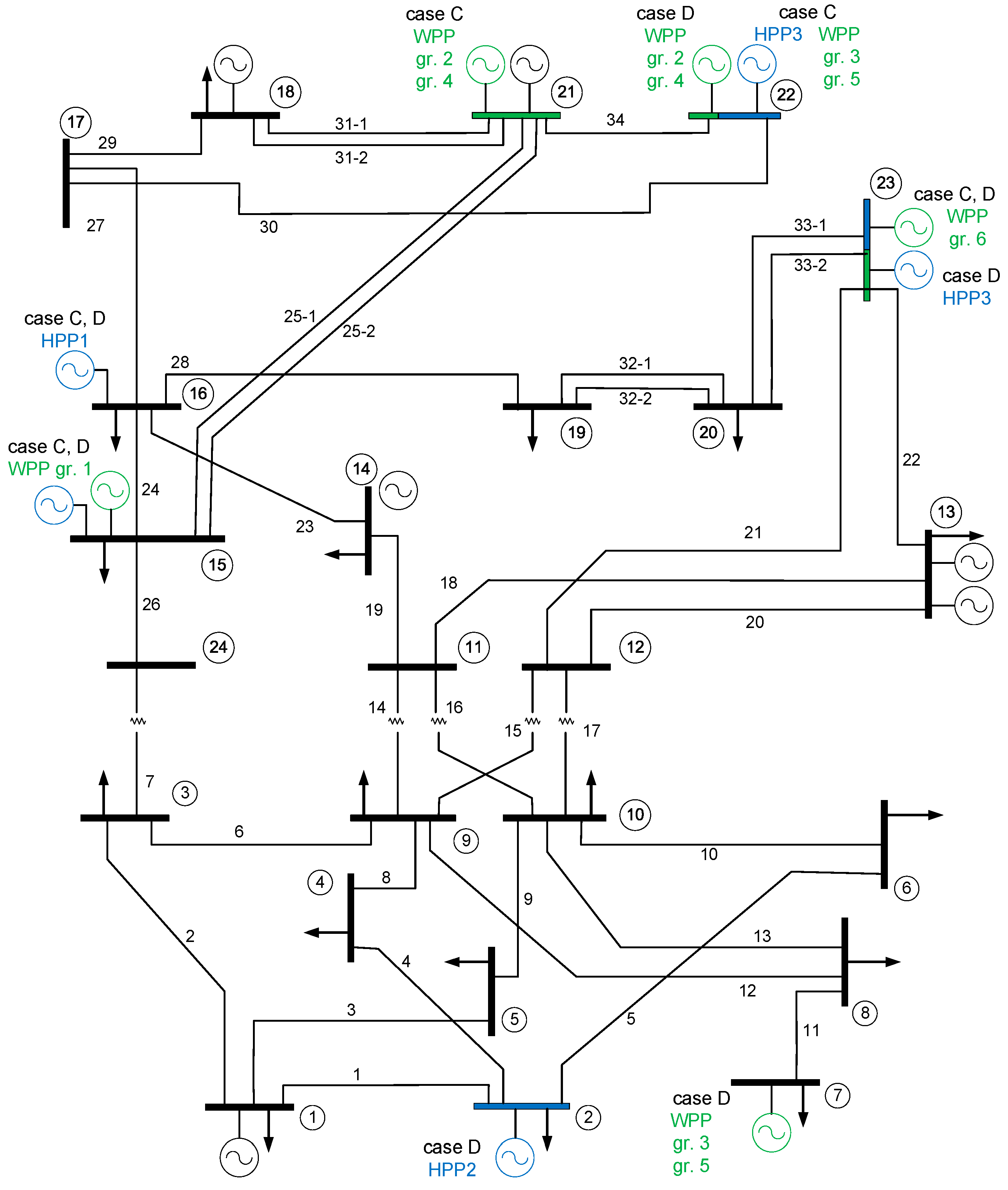
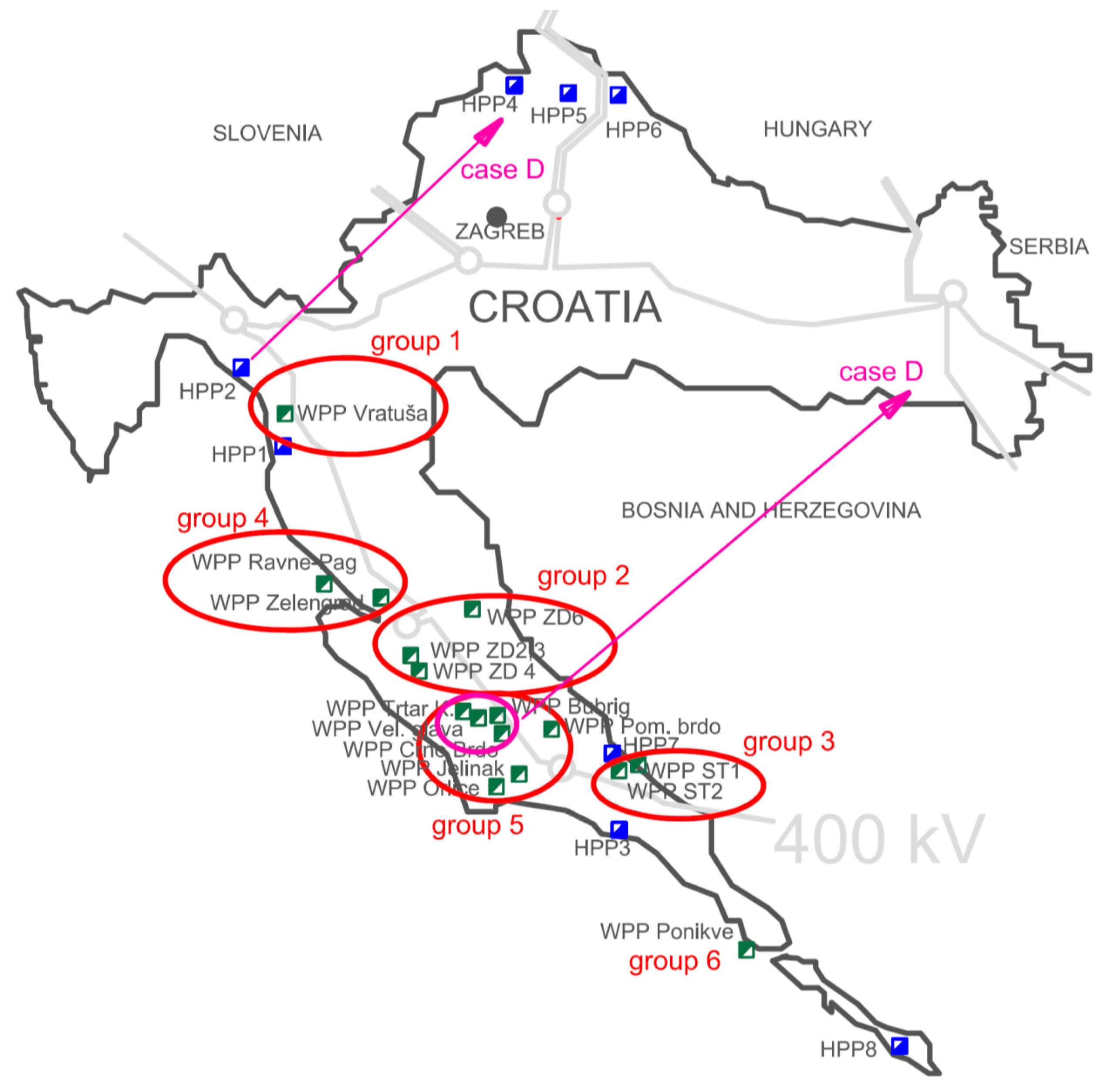
The activation of regulating units due to the power imbalance caused by load or WPP variations also influences the transmission losses. Consequently, transmission losses can be reduced with appropriate scheduling and allocation of regulating units. The aim of this paper is to demonstrate how the dispersion of WPPs with the various errors in generation planning, as well as the dispersion of regulating units, affect transmission losses. The research was carried out with actual operating data from the Croatian control area for typical days in 2015 (different days of the week and different seasons). The tests were conducted on a standard test network RTS 96 [
21] and on the Croatian transmission network for concentrated and dispersed geographical layouts of WPPs and RPPs.
The paper is organized as follows. In the second section, an approach is described for dynamic scheduling of regulating power and determination of the regulating reserve range. The proposed approach improves the regulating reserve scheduling in systems with a large share of wind power, assuring safe operation. With use of the existing daily and hourly load- and wind-power forecasts, the proposed method can be implemented in systems with insufficient historical data, which is the first contribution of this paper. Furthermore, possibilities are discussed for application of advanced information and communications technology. The next section introduces a procedure for optimal allocation of regulating reserves. Minimization of transmission loss is proposed using a combination of differential evolution, a stochastic search algorithm, and power-flow computation using the Gauss-Seidel iterative method. Further possible correction is also proposed based on economic criteria. The following section presents the networks used for testing, i.e., the RTS 96 test network and network of the Croatian control area. The results obtained represent the second contribution of this paper, i.e., the impact that different wind-power generation variations have on the required regulating reserve and on the losses in the transmission system, especially when WPPs and regulating units are dispersed. The next section provides the testing results, while the discussion and conclusions are given at the end.
2. Dynamic Scheduling of Regulating Power
This section discusses a method for dynamic scheduling of regulating power, which is based on the correction of day-ahead schedules, planned using the known variations from the previous hour [
22]. The amount of required regulating power is determined for each successive hour,
h, as:
where
PWPP is the planned power of all the WPPs,
PWPPi is the planned power of the
i-th WPP or WPP group, and
PL is the total load power. The coefficients
kWPPi and
kL are given for the previous (
h − 1) hour, and are defined as the ratio of the actual and planned powers of the
i-th WPP or WPP group and the ratio of the actual and planned load power, respectively.
2.1. Regulating Reserves
Regulating power determined by Equation (1) is used to determine the range of regulating reserve as PRR ∈ [PRR+, PRR−], where the positive and negative reserves are determined as
In order to cover the forecast errors and the sub-hourly variations in the actual wind and load power, safety factors are introduced, i.e., a1, a2 and a3. Furthermore, at sudden changes in the intensity of the wind, the wind power, and therefore, the required regulating power, might change rapidly. In this case, determining the regulating reserve only with data from the previous hour will underestimate the required reserve. By incorporating the tendency of changes for previous hours, the possibility of such cases can be detected, and more regulating power can be reserved at that time.
The range of regulating reserve, PRR, should be different in both positive and negative directions, depending on the sign of the expected amount of the required reserve. When PREG(h), determined by Equation (1) is positive, the positive limit of the range PRR is this sum of PREG(h) increased by a safety factor, a1, and the additional correction part. Then, the negative limit of the range PRR is determined with the safety factors a2 and a3, but at least the Pmin−. When PREG(h) determined by Equation (1) is negative, the positive limit of the range PRR+ should be at least Pmin+ or greater (factors a2 and a3) at sudden changes, i.e., if PREG(h) or its derivative changes the sign. In that case, the negative limit of the range PRR is equal to PREG(h) increased by the safety factor a1, and with an addition of the correction part, but always at least Pmin−.
The amount of the correction part is also variable. A greater value is needed if the time derivative of
PREG has changed the sign, or if it hasn’t changed the sign but decreases, and less value can be added when it is increasing. This is attained by an additional correction term, given as:
where
b1,
b2 and
b3 are safety factors, and
Pmin+ and
Pmin− denote minimum reserves in the opposite direction, whereas the time derivative of
PREG can be approximated with second-order differences as:
2.2. System Operation Safety
In order to assure system operation safety, a sufficient amount of regulating power is required. The minimum values for the positive and negative reserves Pmin+ and Pmin− can be determined as the 70th and 30th percentile of wind- and negative-load-forecast errors, respectively. An entire year should be considered, although it would be desirable to update minimum values for an individual season of the year.
The safety factors a1 and a2 should be between 1 and 1.5, and a3 can be between 0.5 and 1. By increasing the factor a1 on a value greater than 1 (closer to 1.5), the amount of regulating reserve required in the previous hour increases proportionally during the entire day. This is recommended if the share of wind-power is large, however only when the discussed WPPs are not driven by the same wind (not similar weather conditions), i.e., when the variations of generation would be significant, but the sum of those variations can be relatively balanced. Moreover, if the factor a2 is greater than 1, the regulating reserve will be greater in the opposite direction than the minimum for a fixed amount. Factor a3 includes the variable part of the regulating reserve in the opposite direction, when regulating reserve changes the sign, i.e., at sudden wind changes. The higher factor a2 is, the lower factor a3 can be when the wind at the location of WPPs varies gradually, and vice versa, when there are sudden very frequent and irregular changes.
Factors b1, b2 and b3 determine the size of the variable part to be added to the required regulating reserve from the previous hour, depending on the size of these sudden changes of the wind. They can be lower if the WPPs are more dispersed, and, therefore, no extremely large sudden changes occur. Note, if factor a1 is increased, factors b1, b2 and b3 can be decreased, and vice versa. However, b1 and b2 should be between 1 and 1.5, and b3 can be between 0.5 and 1.
The factors discussed should be determined depending on the system specifics and the quality of the forecasts. During this research, an analysis of the required regulating power was performed for the Croatian control area. The measured and forecast data for load power and wind power during 12 selected days in 2015 were used to study their explained relations, and to define the described safety factors. Through graphical analysis of multiple time series, the following optimal values were obtained, i.e., a1 = 1.3, a2 = 1.2, a3 = 0.7, b1 = 1.2, b2 = 1.4 and b3 = 0.5. Using these factors, minimum values of reserved regulating power for each hour were obtained, while the actually required regulating power was within the range [PRR+, PRR−] all the time. When the factors were set to minimal values, as a1 = 1.0, a2 = 1.0, a3 = 0.5, b1 = 1.2, b2 = 1.0 and b3 = 0.5, the actually required regulating power was out of range [PRR+, PRR−] for only nine hours altogether during the 12 days discussed, i.e., 2.5% of the time. This indicates that less positive and negative regulating reserve can be scheduled with better quality of wind- and load-power forecasts.
2.3. Improving Procedure with Advanced ICT Solutions
Although still not included in the method presented in this paper, further improvement of the proposed approach is being developed, that will apply advanced solutions to determine the range of regulating reserve. With the implementation of modern information and communications technology (ICT), the data from the existing software in a dispatch center, as well as the computed results, can be stored in a data warehouse in real or near-real time for future use. By storing the data over a longer period in the data warehouse, conditions for reliable predictions of future corrective factors are created, because the entire system “learns” based on the stored historical data in the data warehouse.
The basic idea for future improvement of the proposed procedure is to make a prototype of the ICT expert system for evaluation of the input parameters. This evaluation can be undertaken independently, or at the request of the user, using data mining methods, with the aim of reducing the mean square error. Among the many available methods and data mining techniques, the artificial neural network (ANN) would be used here [
23], in combination with cluster analysis. This prototype will find appropriate patterns (similar meteorological profiles) and, based on known effects of the former coefficients, form and display appropriate corrections and generate new coefficients for planning the required regulating reserve. The ANN method with adaptive learning finds hidden relationships between input and output data, i.e., it finds hidden data patterns to achieve new comprehension of the data collected in the past.
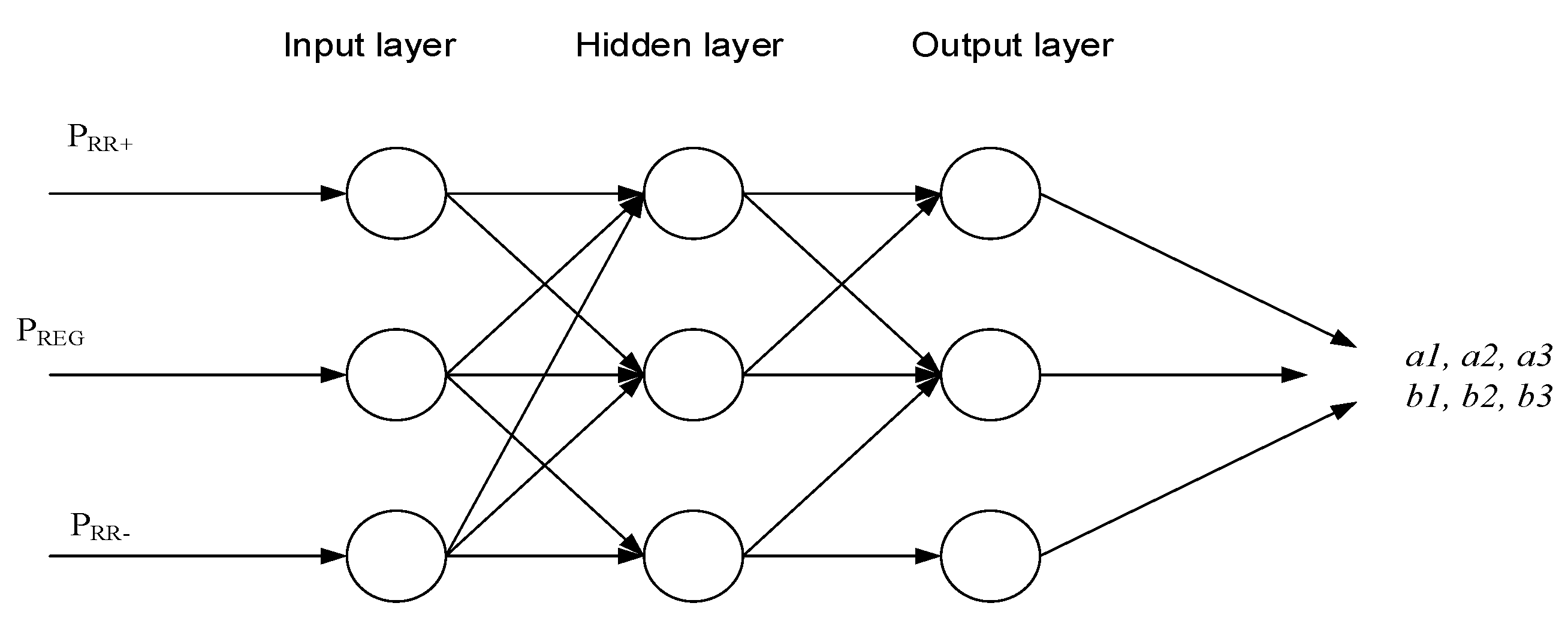
The modeling of ANN usually begins with an input layer, with one or more hidden layers and one output layer, although there is no standard ANN architecture. In view of the specific application, a suitable form of network and pattern for processed information is selected and presented in a vector form. In the approach proposed in this research, the inputs to the individual layers are the amounts of required regulating power
PREG, and the upper and lower power limits (
PRR+,
PRR−) per hour within a day. The expected outputs from all layers are the corresponding corrective parameters for planned regulating reserve in the future period, as is shown in
Figure 1.
3. Allocation of Regulating Power
In order to create the proposal for allocation of the reserved regulating power in a set of available regulating units, the optimization procedure is proposed using differential evolution. This procedure includes the differential evolution algorithm in combination with the power flow computation using the Gauss-Seidel iterative method.
The following assumptions and limitations are included in the proposed optimization model: Operating reserve planning is limited to regulating (secondary) reserve planning; distribution of the regulating reserve is optimized according to minimum transmission losses; hourly-based states are discussed, and the correlation between load and wind power is neglected. In order to perform the computations, network configuration and network state estimates have to be available, as well as load consumption and wind-power generation, and the day ahead forecast for load and wind-power.
3.1. Differential Evolution Algorithm
The differential evolution (DE) algorithm [
24,
25] is often applied for optimization problems in electric power systems. DE is a stochastic optimization algorithm, which has proved very robust in solving realistic technical problems, i.e., it avoids the local minimum towards the global minimum. It is simple, easy to implement, and requires no particular starting point. Therefore, it is suitable for solving global optimization problems with nonlinear constraints [
26,
27,
28], and it has been used in all of the optimizations in this research [
29].
In this paper, the objective function is set to minimize active power losses in the transmission system with respect to the technical limitations of network components. After the DE algorithm is started, the optimization parameters are entered (strategy, step size F, crossover probability constant Cr). Next, the initial elements of the population are generated by a random method (initialization phase). This is followed by mutation, recombination, and selection of the elements for the next iteration. The selection of the elements (members of the population) is executed for each vector through a combination of random, or random and the best value from the previous iteration, values depending on the chosen strategy. The algorithm returns the best-attained value, and the members of the population to which the best value applies, when the desired accuracy is achieved (or after a preset maximum number of iterations). The described optimization algorithm is implemented in the procedures for transmission-loss minimization and allocation of regulating reserves.
Different optimization parameters and strategies were used during the tests without significant influences on optimization results. Therefore, the typical values were used, i.e., F = 0.7 and Cr = 0.5.
3.2. Power-Flow Computation
Gauss-Seidel (GS) and Newton-Raphson (NR) are iterative numerical methods that are used most commonly for AC power-flow computations [
30]. GS is the method of successive displacement for solving the linear system of equations with iterative techniques. It is quite easy to program, and one iteration is done very quickly, but the number of iterations increases with the number of nodes in the network [
31,
32]. The NR method uses equations in polar form and the iterative process to find the approximation of the root of a function. This method is more popular, because it has better convergence, however, depending on initial values, large oscillations may occur [
32]. The equations in NR are more complex, and the duration of one iteration is longer, but it needs fewer iterations to solve them. Generally, GS requires a larger number of iterations, but the computations are simpler, and that is why the GS method converges, even for larger variations. In this work, power flow computations were carried out with the GS method which was determined as being more suitable because of the large variations in nodal generation. Therefore, this method will be presented here in more detail.
The voltage phasor for the
p-th node is determined for the
k-th iteration by:
where
N is the number of all the independent nodes, (•)* denotes the complex conjugate. The constant,
Kpi, is given by the ratio of the admittances (
Ypi/
Ypp).
Kpp is given by the ratio of the nodal apparent power and the admittance (
Sp */
Ypp), taking into account the load power, the power from all the power plants, including RPPs and WPPs, as well as the scheduled interchange power on the area’s tie-lines.
In order to maintain the nodal voltages within the prescribed limits, the reactive power is corrected, which for the
p-th node and
k-th iteration are determined by:
When Qp(k) < Qpmin then Kpp is recalculated using Qpmin, whereas when Qp(k) > Qpmax, then Qpmax is used instead. Note that the reactive power correction is only applied to nodes with voltage regulation. The computation is repeated for all the nodes with satisfactory accuracy, or to a given maximum number of iterations.
The power flow through a transmission line, e.g., between the nodes
p and
q, is determined by:
where
Ipq is the current phasor and
Bpq denotes the shunt susceptance. The transmission losses on the line
p-
q are determined as Re{
Spq −
Sqp}, whereas the total transmission losses,
PLOSS, are calculated as the sum of the losses on all the lines.
3.3. Transmission-Loss Minimization and Regulating Power Allocation
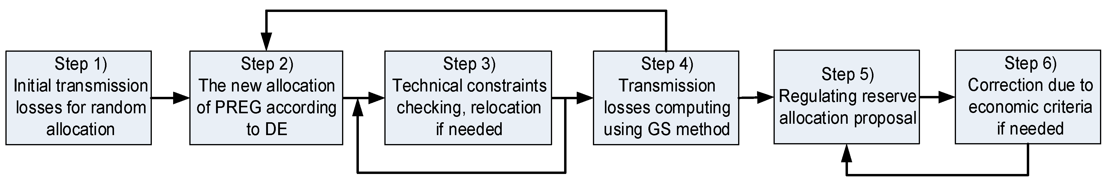
Load variations were monitored over many years in all the power systems. Therefore, the load forecast error is mostly very low (1% to 2% in Croatia) and dispersed evenly over the entire network. On the other hand, variations of renewable energy sources cannot be predicted very precisely, especially in systems where their share is changing (increasing) every year. Furthermore, wind power forecast error (WPFE) can vary significantly from one WPP to another. Considering this, RPPs should compensate for the deficit/surplus of active power, caused either by load variations or by WPFEs. That is the task of the load-frequency control (LFC). Furthermore, changes of power flows in the network are dependent on the node in which the generation of regulating power is increased or decreased, and where the load and generation from renewable energy sources are increased or decreased. Then, changes in the generation of reactive power, i.e., Voltage/VAr Control (VVC) are carried out in order to retain the voltage in all nodes within the prescribed limits. Yet again, VVC also exists only in some nodes, so the power flows have to be recalculated. This is the reason why the optimization and power flow computations must be intertwined. The proposed procedure is presented as a block diagram in
Figure 2, and described further in Reference [
33].
3.4. Economic Features
The proposed allocation of regulating units can be corrected with economic criteria following optimization with technical criteria, as is shown in
Figure 2. Four main groups of the relevant economic features of ancillary services markets, each with four different approaches, were analyzed and summarized by the authors of [
34]. The qualitative analysis of those features was undertaken and presented in Reference [
33]. Depending on the procurement and remuneration method of ancillary services, as well as on the structure of the remuneration, a greater or lesser need is expected for assessing the impact of the economic criteria. Furthermore, the criterion of minimal transmission losses is dominant for some of the approaches, while for other approaches, lower prices of offered ancillary services or generation from different regulating units can be important too. The other economic features, such as frequency of review of needs, duration of contracts for provision of ancillary services, or market concentration of regulating units, will have an influence on the quality of the optimization. The best solution would be the co-optimization of energy and ancillary services, even though it is rarely possible.
5. Results
The tests were carried out with hourly planned and realized wind and load power captured in the Croatian control area. Twelve representative days in 2015 were selected, taking into account working days, weekends and holidays during the spring, summer, autumn and winter [
22].
5.1. Comparison of the Proposed and Classic Approaches to Reserve Scheduling
A classic approach is still used in the Croatian control area, which does not account for the fluctuations in generation from WPPs. The tertiary reserve is set up mostly on 80 MW throughout the whole year. The secondary reserve is determined as the minimum recommended amount, i.e., between 35 MW and 75 MW, depending on the maximum anticipated load during the day and for a different month of the year [
29].
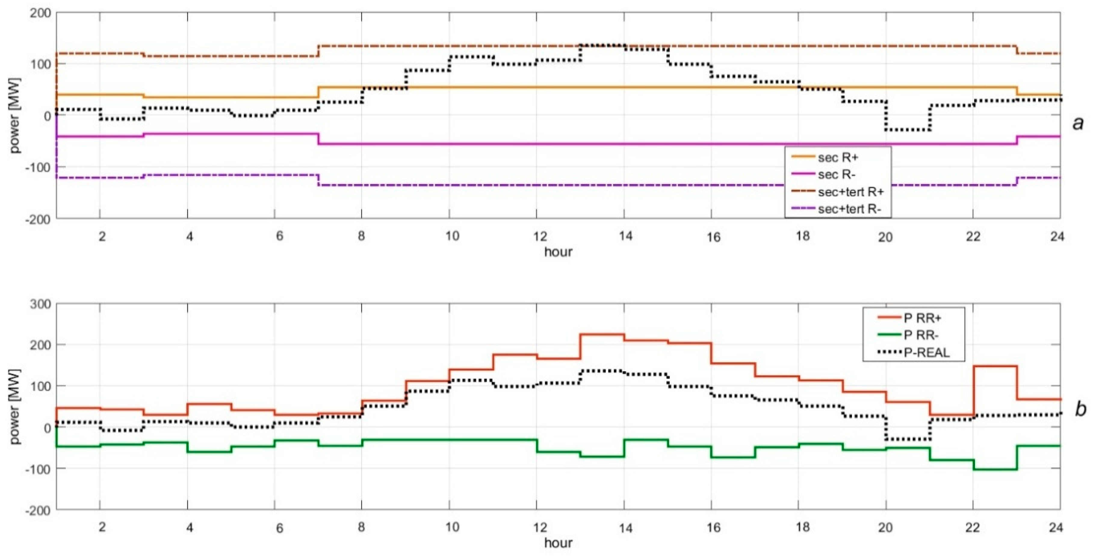
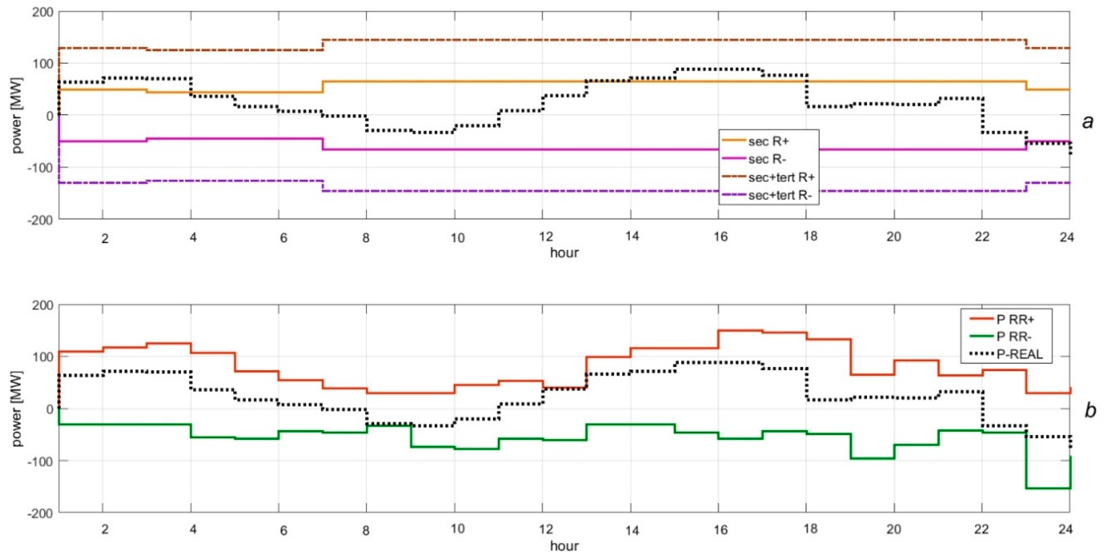
Results are shown for two selected days.
Figure 5a and
Figure 6a show reserve power for secondary and tertiary regulation determined by the classic approach.
Figure 5b and
Figure 6b show the positive and negative reserve power (
PRR+,
PRR−) determined by the proposed approach, i.e., dynamic scheduling, using Equations (1)–(3). Furthermore, the actually needed regulating reserve is also shown (P-REAL), which was calculated with known values for the planned and realized generation and consumption in the
h-th hour. It can be seen that the actually needed regulating power is always within the range of the scheduled positive or negative regulating reserve calculated with the proposed approach. According to the classic approach, the required regulating power was often out of range of the scheduled secondary reserve in either a positive or negative direction (sec R
+, sec R
−), and even occasionally out of range of the scheduled secondary plus tertiary reserve (sec+tert R
+, sec+tert R
−).
5.2. Transmission Losses
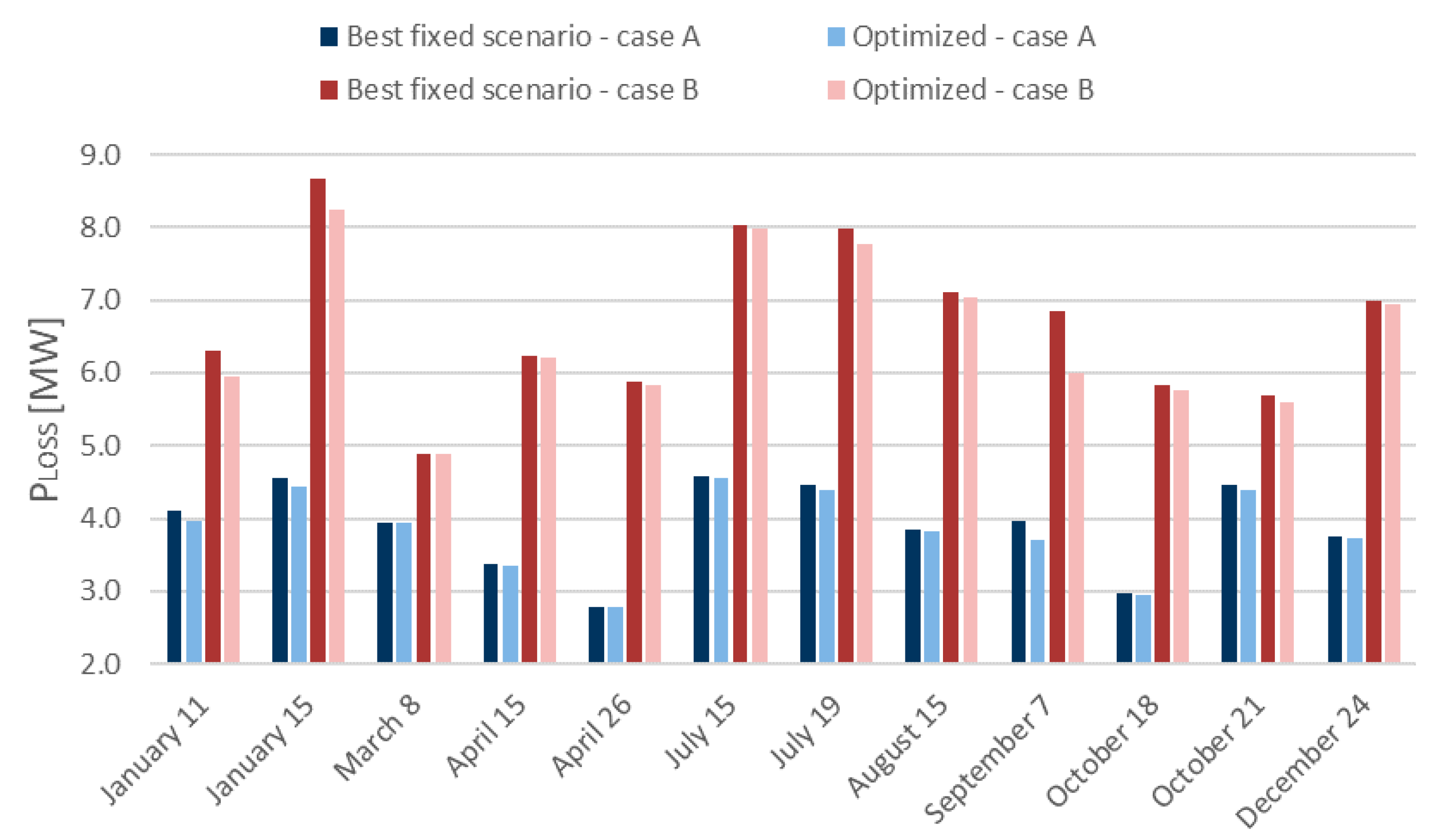
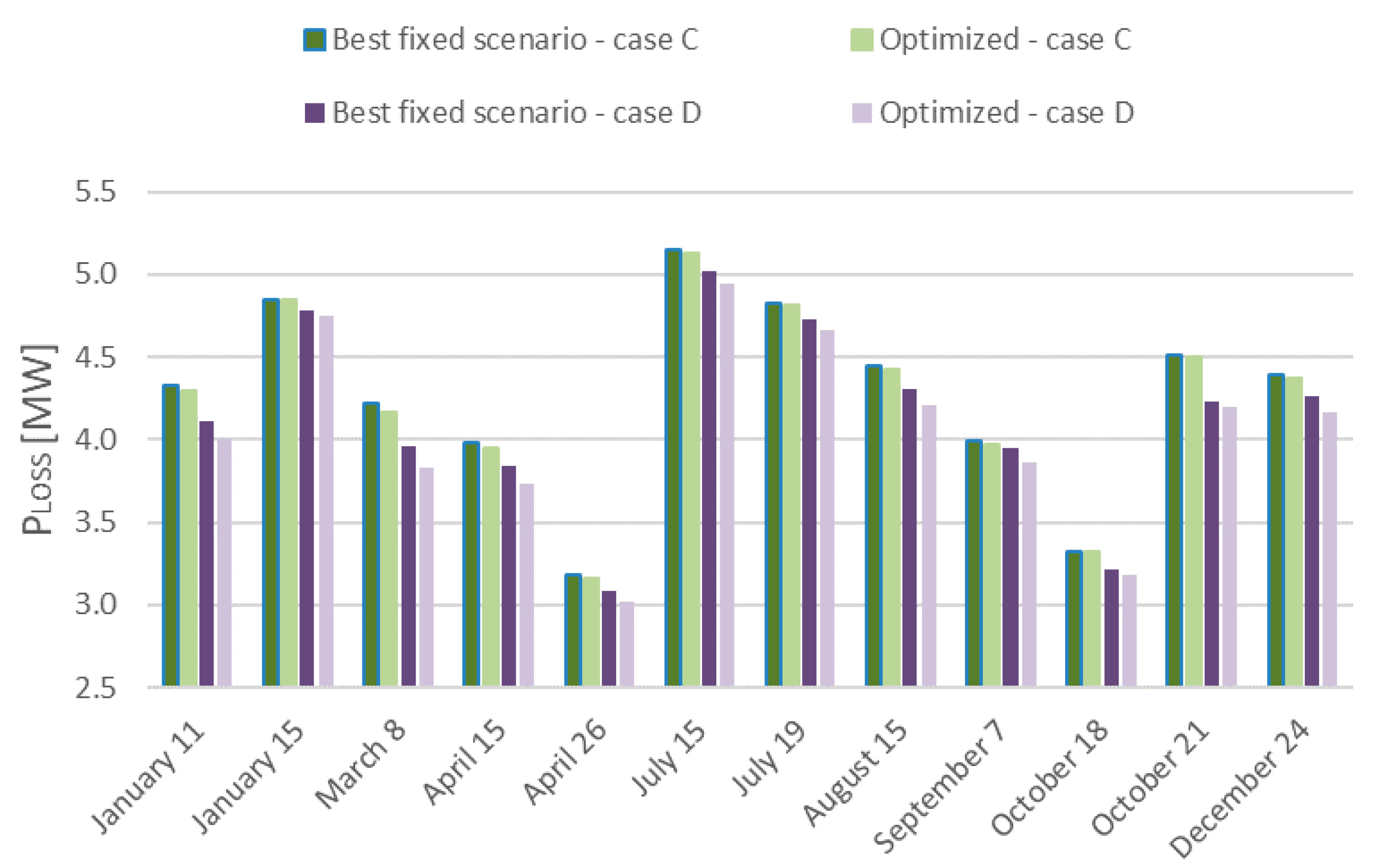
For all four case studies (A–D), actual data from the Croatian control area were used, obtained for each hour of 12 selected days in 2015. Thereby, the optimal allocation of regulating units was obtained, as well as the total transmission losses, using the proposed procedure. Furthermore, three fixed scenarios often used in Croatia were also considered, when one or another regulating unit is ready for regulation. The most common is the third scenario, where only HPP2 is ready during the night and HPP1 has priority in the negative direction, HPP3 has priority in the positive direction during the day, and, if more power is needed, the other HPPs will participate in the LFC.
The optimal distribution was different for every hour and every day, depending on the forecast error of individual WPPs. When the location between the WPPs and the regulating HPPs was geographically close, lower transmission losses were achieved with activation of the regulating HPP that is nearer to the WPP with the highest wind-power variation. The reduction of transmission losses when applying the optimal allocation of regulating units, compared with the discussed fixed scenarios, was different for each of the days in each scenario. The achieved loss reductions in the Croatian control area were not high, due to the relatively small share of WPP generation (10%) and the close geographical locations of the WPPs and the regulating HPPs. Furthermore, such small decreases of transmission losses, when compared with the often-used scenarios, can indicate good and experienced practice in classic reserve scheduling. The comparison between the daily losses obtained for a fixed scenario with the lowest total transmission loss values and for optimal allocation is presented in
Figure 7 and
Figure 8 for all discussed cases (A–D).
For the tests on the RTS 96 network in case A, loss reduction could be almost 7%, but, on average, the reduction was 1.56%. However, for more dispersed locations (case B) the loss reduction could be even more than 12%, although the average reduction was 2.61%. For the Croatian network, the best scenario was the third scenario, which is the most commonly used in praxis. For case C, the reduction of losses was slightly over 1%, with an average value of 0.49%. However, for more dispersed locations of the regulating HPPs and WPPs (case D) the reduction could be more than 3%, while the average value was 1.92%.
5.3. Computation Time
The proposed optimization procedure realized as a prototype implementation in Matlab R2012a, was run on a 3.3-GHz Intel Core i5-3550 with 8 GB of RAM. The elapsed computation time was approximately 35 min for the next 24 h in the tested Croatian control area. The computation speed is not crucial, since the allocation proposal is intended for day-ahead reserve planning and not for online regulation.
6. Discussion and Conclusions
The proposed approach improves the scheduling of the required regulating power in control areas with a large share of WPPs. Moreover, it ensures easy implementation in the systems with insufficient historical data, by requiring only available operational data. Consequently, the costs for regulating power are reduced, while the system operation safety is increased. The savings in regulating power costs obtained were substantial for the selected 12 days, and can be increased further by implementing modern ICT technologies. The possibilities for improvement of the proposed approach and the quality of the obtained results are directly dependent on the amount and quality of data available from the electric power transmission system. Furthermore, a minimization of transmission losses was also discussed. A relatively small reduction of transmission losses compared with the often-used scenarios in Croatia may indicate good and experienced practice in reserve allocation. In addition, the results obtained showed that the optimization of regulating power allocation has significantly greater impact in networks with more dispersed WPPs and regulating units. This indicates the importance of analyzing the impact of reserve allocation on the transmission losses when planning the construction of new WPPs and regulating units, as well as within daily operation planning procedures. There are natural extensions for the work presented in this paper. The proposed dynamic scheduling can be enhanced with the ANN with deep learning, which is possible by storing the data during a longer period. Furthermore, in the systems where the regulating capacities have different costs per unit, the proposed method for allocation of regulating reserves should also contain a correction algorithm which includes the economic criteria.


