Article

Partial Shading Detection and Global Maximum Power Point Tracking Algorithm for Photovoltaic with the Variation of Irradiation and Temperature

Graduate School of Engineering and Science, Shibaura Institute of Technology, Tokyo 135-8548, Japan
*
Author to whom correspondence should be addressed.
Energies 2019, 12(2), 202; https://doi.org/10.3390/en12020202
Submission received: 7 November 2018 / Revised: 5 January 2019 / Accepted: 5 January 2019 / Published: 9 January 2019
(This article belongs to the Special Issue Sustainable Energy Systems)

Abstract

:
Photovoltaic (PV) technology has been the focus of interest due to its nonpolluting operation and good installation flexibility. Irradiation and temperature are the two main factors which impact the performance of the PV system. Accordingly, when partial shading from surroundings occurs, its incident shadow diminishes the irradiation and reduces the generated power. Since the conventional maximum power point tracking methods (MPPT) could not distinguish the global maximum power of the power-voltage (P-V) characteristic curve, a new tracking method needs to be developed. This paper proposes a global maximum power point tracking method using shading detection and the trend of slopes from each section of the curve. Full mathematical equations and algorithms are presented. Simulations based on real weather data were performed both in short-term and long-term studies. Moreover, this paper also presents the experiment using the DC-DC synchronous and interleaved boost converter. Results from the simulation show an accurate tracking result and the system can enhance the total energy generated by 8.55% compared to the conventional scanning method. Moreover, the experiment also confirms the success of the proposed tracking algorithm.

1. Introduction

Research in renewable energy has recently received great attention. Especially for photovoltaic (PV) technology, renewable energy has gained popularity as one of the potential avenues due to unlimited power resources and unpolluted operation [1]. To enhance the efficiency of PV, the effect of weather conditions must be considered. According to research by Patel and Agarwal [2], there are two main parameters which affect the PV-generated power, irradiation and temperature; where PV technology is installed, the generated power varies from location to location. It is apparent that we cannot control the two aforementioned parameters; therefore, the problem of “PV mismatch” can occur.
PV mismatch is defined as the difference between the expected and actual output power from a PV module, causing difficulties in PV technology generating power. Classified according to its source, mismatch can be internal or external. If PV power degradation occurs due to the quality of the panel, such as aging and impurities in the Silicon crystal, the mismatch is considered internal as it stems from the material’s properties, and product replacement can solve the issue. However, if degradation occurs due to an environmental factor, mainly shading from PV alignment and the surroundings, the mismatch is considered external. The effect from shading has also been pointed out by Femia et al. [3] and Gao et al. [4] who considered shaded PV panel a significant obstacle in the rapid growth of solar PV systems. The study by Eftichios et al. [5] offers a practical case study through PV rooftop systems in Germany, where 41% of the installed panels had been affected by shading, with energy losses up to 10%. Hence, remarkable reduction of power generated was observed. In the same manner, Daraban et al. [6] presented a case study of 13 different PV power tracking systems operating under a shading condition, where the result showed up to 70% of power was a loss due to not detecting the actual maximum power.
In electrical engineering, PV operating current and voltage form a non-linear relationship, demonstrated as the current-voltage (I-V) and power-voltage (P-V) characteristic curve. Figure 1a,b presents the series-connected PV array operated at a normal condition and with partial shading. Here, the bypass diodes were installed on each panel and a blocking diode was installed on each PV branch to reduce the effect of shading [2,7,8]. The I-V and P-V characteristic curves corresponding to each condition are shown in Figure 1c. Here, we can observe the significant difference between the two conditions is that shading exhibits multiple local peaks, while the normal condition shows only a single peak. Naming each peak as the local power peak with the highest among all points as the global power peak increases the challenge for the maximum power point tracking (MPPT) system to locate the correct global power peak point [2,9,10,11].
Under shading conditions, it has been confirmed by previous research that conventional MPPT methods fail to ensure successful and precise tracking of the global power peak [6,9,10,11,12]. Consequently, the difficulties in implementing MPPT include the complexity of the algorithm, cost, and failure while operating in shading conditions [5]. Studies of global power peak identification under shading conditions have been done, especially in the past five years; each study presented a tracking method with a variation of complexity, cost, operating speed, and range of effectiveness [12]. These variations should be taken into consideration when designing an effective MPPT system [4].
Mainly, previous MPPT techniques can be distinguished into two categories, differentiated based on the method of implementation. The first category originates from the improvement of the existing conventional tracking method; these include the well-known MPPT techniques but with further modification (for instance, perturb and observe (P&O) and incremental conductance (InC) [13]). Research in References [14,15,16,17] confirms the effectiveness of the conventional methods that can locate the correct global power peak. The second category istopologies based on the intelligence computing method. Since 2015, these intelligence methods have been used to solve the maximum power point (MPP) tracking problem under the shading situation. Examples include the fuzzy logic-based MPPT, artificial neural networks (ANN), and the artificial bee colony presented by Bidyadhar et al. [18] and Kinattigal et al. [19].
Focusing on the conventional method, Reference [14] guarantees that scanning could locate the global power peak, and the region the local power peak should be established between 75% to 80% of PV total open circuit voltage ( V O C ) . By setting the scan point as the multiple of 75% of the PV module open-circuit voltage, the global power peak can be obtained. However, the disadvantage is the requirement of samples and the tracking time consumption. Studies have continued to investigate other tracking methods without scanning the whole P-V characteristic curve, for example: The presented work by Eftichios et al. [5] shows how the global MPPT methods work by distributing PV load lines on the characteristic curve and reference points are indicated along these lines. The result shows the complete tracking results with higher efficiency compared with the PV scanning and particle swarm optimization (PSO), which is one of the optimization methods that can be a solution for the optimization problem using the concept modeled after bird folk’s behavior. Nonetheless, the work does not provide the time response result, and the implementation requires additional switching circuits, such as a flip-flop and a comparator.
The research performed by Hiren [20] shows the remarkable tracking algorithm by setting the threshold to detect changes of power when shading happens and using the change of power concerning the voltage d P d V to determine the tracking direction. The tracking algorithm was confirmed to be effective, but the simulation showed the result only in short-term, with the practical long-term result for more than 30 seconds not indicated. A similar prospect presented in Reference [4] also used the slope calculation trend of the P-V curve to indicate the peaks for small-scale PV devices. The result confirmed the success in tracking after tests lasting up to one hour during a rapid change of irradiation; however, this study does not present the analysis for medium to large scale PV systems with a capacity more than 1 kW.
The proposed method by Jubaer [21] discussed the disadvantage of P&O algorithm due to its oscillating response when operating in rapid irradiation change. The paper also proposed equations to detect power deviation, which are used together with the tracking algorithm; however, the computation contains many checking parameters which complicate programming, and the paper does not focus on the long-term operation principle. Further research by Korey [22] presents global MPPT tracking based on P&O, experimented with three PV panels connected in series. The results showed successful tracking, but oscillation still existed, and the quantity of the power generated was not analyzed. Research by Alik et al. [14] used the concept of P&O with an additional checking algorithm to track the global MPP. The simulation was tested for the short-term changes om irradiation; however, it did not mention the changes in temperature and practical experiments. Additionally, the proposed variable step perturb and observe (PO) and global scanning method (VSPO&GS) method by Duan et al. [16] contributed more tracking speed and accuracy. The drawback is that the simulation result was not compared with other conventional or global MPP methods; as a result, its efficiency could not be determined. The research by Başoğlu [17] proposed an excellent concept for improving, scanning, which included the “full scanning” and “large scanning” methods. Both methods limit the scanning interval, shortening it, and can guarantee the effectiveness of the algorithm, but similar to other reviewed papers, long-term testing was not presented, except for Reference [20], which supports the ineffectiveness of the conventional tracking method, which cannot guarantee the accuracy of MPPT during shading conditions. The algorithm proclaims the first tracked peak as the global MPP until the change of irradiation and temperature happen, causing the tracking error in the system.
In order to simplify the complicated tracking system, there is a number of previous studies that present interesting aspects. Developed by Kobayashi et al. [23] and Irisawa et al. [24], two-stage maximum power point tracking control is proposed. In the first stage, the optimum operating point of the PV system is controlled to converge the MPP; afterward, the second stage operates to move closer to the real MPP. The work still faces the same problem when operating under some non-uniform irradiation conditions. Moreover, an additional control circuit is also required. Alternatively, Bekker [25] presents the optimal MPPT method using the open-circuit voltage sweep along the P-V curve, but the loss from tracking is still present. The method by Nguyen [26] shows the adaptive reconfiguration scheme to reduce the effect of shading; consequently, the switching matrix is connected to the adaptive solar bank. The result confirms the real-time operation; however, this requires additional switches and sensors in proportion to the size of the PV array. Reference [27] proposes control topology for the bidirectional DC-DC converter implemented in parallel connection, where the objective is to reduce the effect of shading on the other PV modules. However, the drawbacks are the requirement of extra hardware and additional cost. Finally, Uno [28] presents the current-sensorless and Δ V-controlled optimization in order to reduce the number of switches and sensors in the system. Only the additional control system for the gate driving system is necessary.
As for other intelligence tracking methods proposed in many research papers, they show the guarantee for tracking MPPT in shading conditions. Nonetheless, the significant disadvantages of the intelligence technique are the requirement of additional circuits, the added complexity, and high implementation cost [4]. Research by Yuan [29] proposes adaptive inertial weight particle swarm optimization (AWIPSO) based on the original PSO method. The method has the flexibility to adjust weight coefficient parameters, which can increase the speed of tracking. The algorithm was confirmed using the simulation; however, the experimental results were not included. In References [30,31,32], MPPT from a PSO approach was also demonstrated, which shows the accuracy from the simulation and experimental results. Nonetheless, the work by Miyatake et al. [30] requires a separate converter per one module, causing the extra cost. Additionally, using PSO, the first difficulties are the calculation for the related variables, precision in setting, and the requirement of cooperative agents and learning factors [10,32]. Apart from PSO, Alajmi et al. [33] present how a modified fuzzy-logic controller can be implemented. Correspondingly, the design is based on a diode model equation of the PV panel, combining with the modified fuzzy-logic from the hill-climbing method. However, the system requires thirty-two fuzzy control rules, which add more complexity to the system.
In practice, most of the commercial PV inverters used in PV installation used the scanning, P&O and InC algorithm to track the maximum power point [10]. From the technical specification of PV inverters, scanning is set to be every 15 min of the time interval [34,35]. The problem with this topology is that it is difficult to predict the irradiation and temperature changes in a day. The scanning interval might not match the weather conditions. By choosing a long scanning interval on the day with the rapid change of weather, tracking error may occur due to the mismatch of the selected interval. Additionally, by choosing a short scanning interval on the day with a steady change of irradiation and temperature, power loss from the unnecessary tracking is achieved. Similarly, the scanning requires tracking time, which leads to more power loss [36]. As a result, the main properties established to implement successful MPPT in shading conditions should include high efficiency and simple implementation [19]. Previously reviewed research presents the analysis of conventional scanning for commercial inverters and its weakness when the setup does not match the weather conditions. Although the system includes the blocking and bypass diodes to prevent heating and damage, the considerable decrease of power from shading still occurs.
This paper presents the original idea of studying the patterns of the P-V characteristic curve to design the new tracking method. Studies of I-V and P-V characteristic curves from several PV panels are simulated. The I-V curves are used to study the relationship between the irradiation and PV current in order to design the shading detection algorithm (the full explanation of the methods is in Section 3.2.2), whereas the P-V curves are used to design the MPP tracking (explained in Section 3.2.4). Although these patterns vary due to many factors from different PV module specifications, the typical pattern among the curves was found. The proposed algorithm uses the simple concept of mountain climbing to search the mountain’s peak, in order to locate the local and global power peaks without scanning the whole curves. This idea is new and not shown in other papers. Moreover, in order to evaluate the performance of the tracking algorithm, it is suggested by Miyatake et al. [30] to use the real measured data and test for several hours. Since most of the papers on MPPT show only the short-term response and focus on the time used for tracking, in this case, the author uses real weather data from the author’s institution to perform a long-term case study [37]. In conclusion, this paper’s contribution includes the following advantages:
  • The accuracy of global MPP tracking;
  • the fast-tracking time with less tracking power loss compared to the conventional scanning method;
  • the ability to operate at dynamic changes of shading and weather conditions;
  • no irradiation and temperature sensors required;
  • no additional control circuits required;
  • simple switching control using the centralized converter;
  • simple control topology compared to the intelligence tracking methods .
The usefulness of this research is that the proposed algorithm can be used to track the PV power in both ordinary and partial shading conditions. Additionally, the implementation can be done with the conventional DC-DC boost converter, meaning it can be used in practice for small- to medium-scale PV array. The proposed algorithm is described using mathematical equations with flowcharts and examples for better understanding.

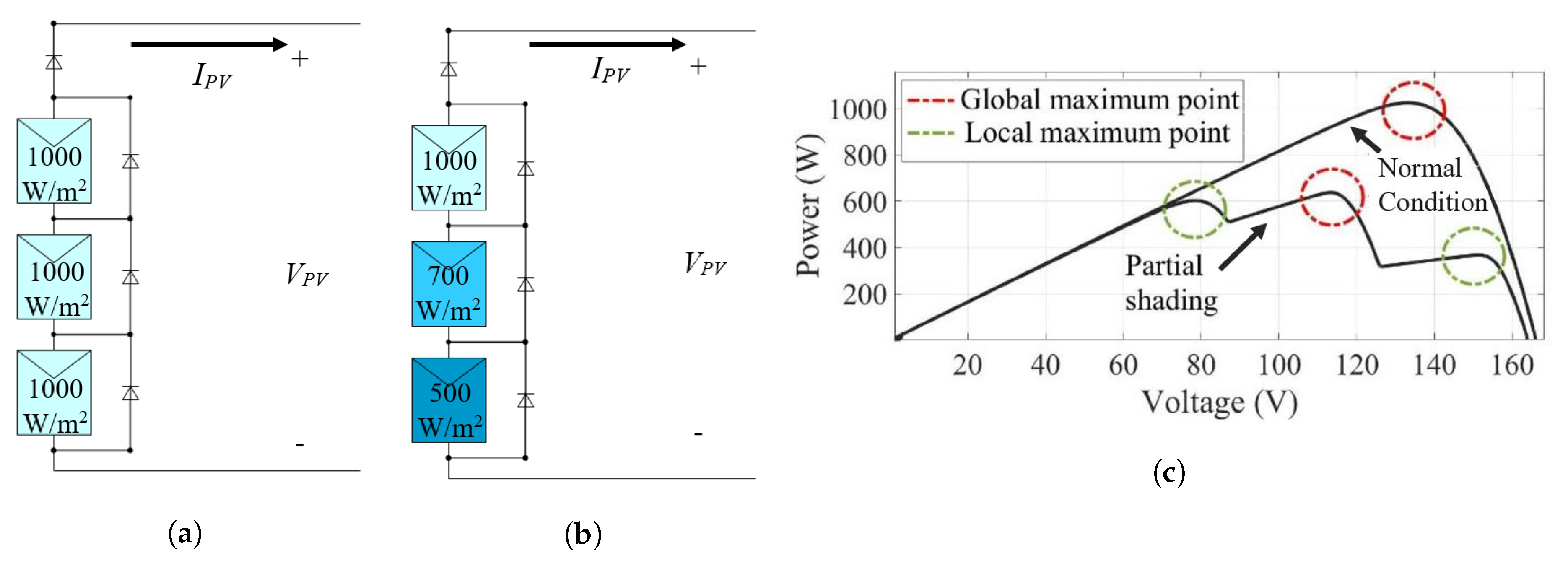
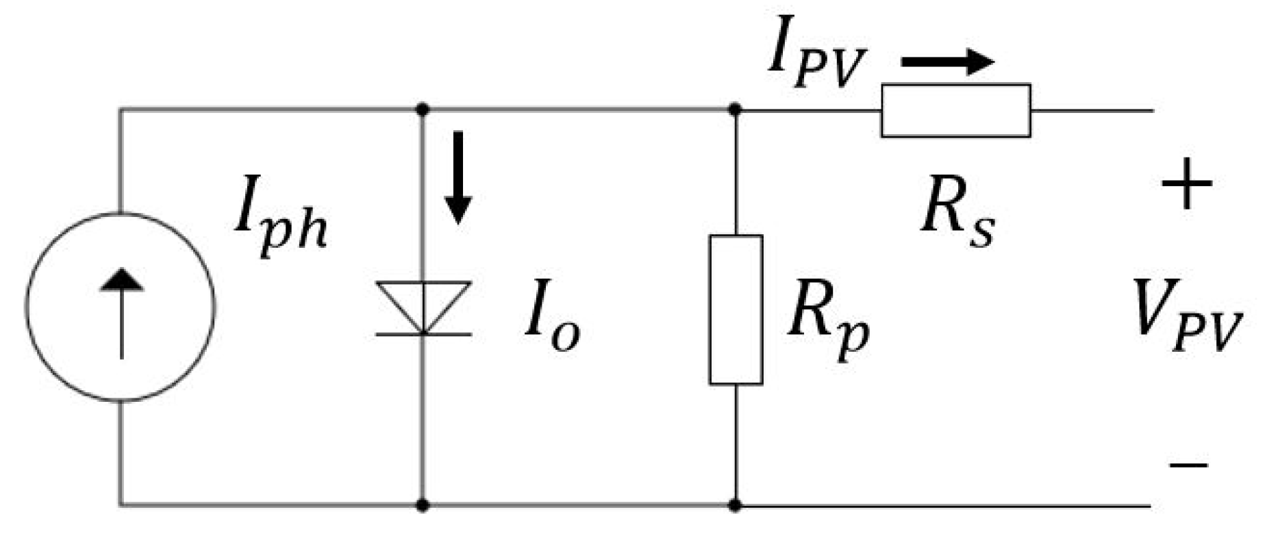
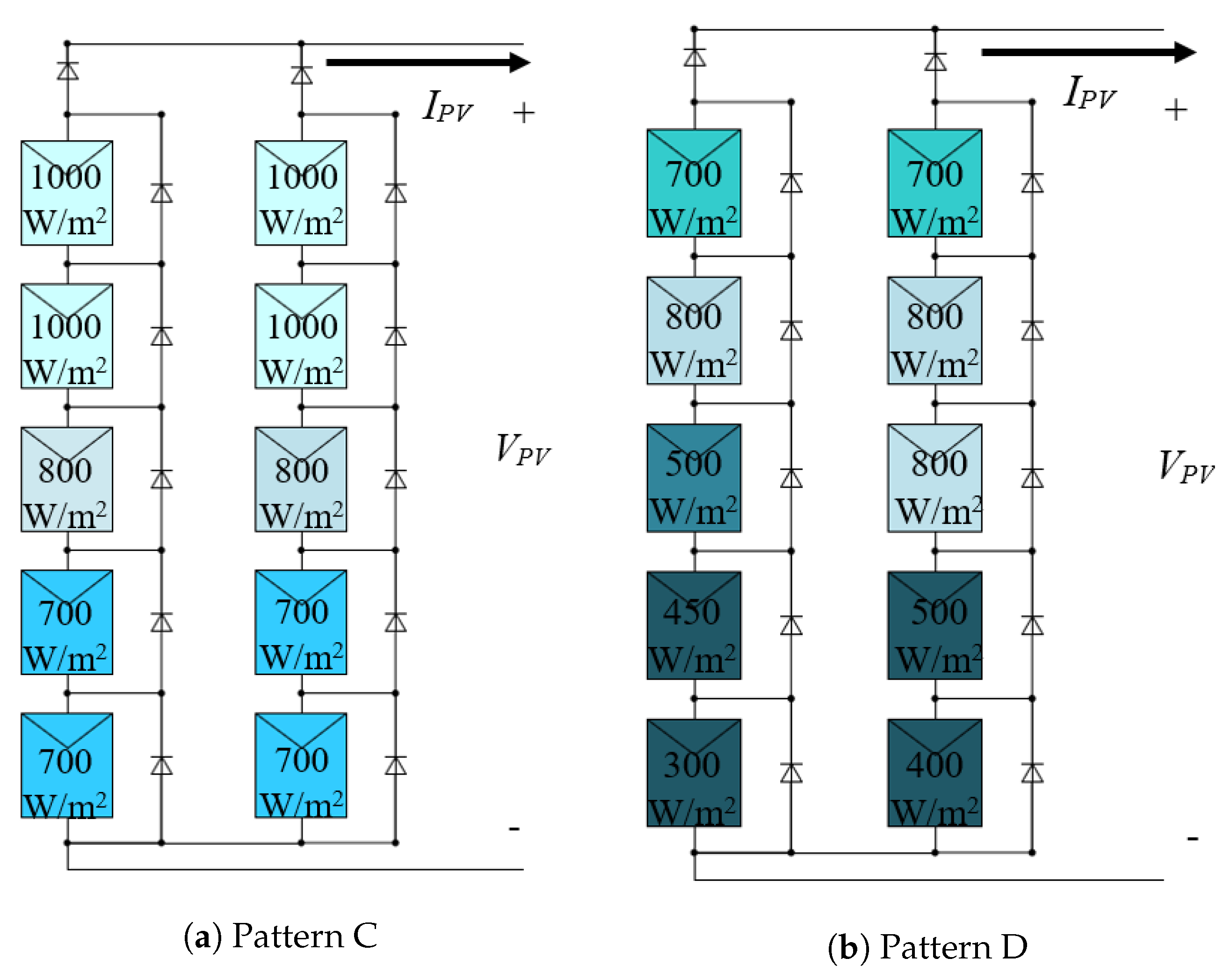
2. Partial Shading Condition for PV Systems

An ideal PV module can be modelled as a single diode equivalent circuit [38]. Equation (1) represents the mathematical relationship between the PV module current I P V and other related parameters [39]. Figure 2 shows the single diode equivalent circuit, including a current source I p h connected antiparallel with a diode, including series resistor R s and parallel resistor R p .
I P V = ( I P V , S T C + K I Δ T ) G G n
From Equation (1), I P V , S T C is the PV’s current of the module in standard test conditions (STC), K I is the temperature coefficient of current, G is the solar irradiation measured in W / m 2 and G n is the nominal solar irradiation (1000 W / m 2 ). From the equation, we can observe the directly proportional relationship between G and I P V , S T C in that the higher the irradiation, the more PV current is measured. However, when irradiation decreases due to shading, the current reduces. In addition, Equation (2) represents the calculation of the PV module’s open-circuit voltage ( V O C ) [20]:
V O C = V O C , S T C + K V ( T T S T C ) + a V T ln ( G G S T C ) ,
where V O C , S T C is the PV module’s open-circuit voltage, K V is the temperature coefficient of voltage, T represents temperature and T S T C is the temperature at STC (25 °C). Additionally, a is the diode ideality constant and V T is voltage constant. It is shown in the equation that open-circuit voltage varies with both irradiation and temperature; by assuming the last term of Equation (2) to be very small, the temperature level is the primary cause for the variation of PV’s open-circuit voltage value. Likewise, it is shown from Equations (1) and (2) that the operation of PV varies with irradiation and temperature [40].
In order to design an effective MPPT algorithm, more than 20 samples of P–V characteristic curves were analyzed. Figure 3 shows series-connected PV modules with different patterns of irradiation and temperature, specified as pattern A and B, where the temperature for each pattern is 25 °C and 30 °C, respectively.
Regarding the review states in the introduction, conventional MPPT algorithms cannot distinguish the local and global maximum point existing on the P-V characteristic curve; this contributes to the complexity in tracking the correct maximum point. Additionally, a variation in PV current and voltage happens to the system when there is partial shading, causing the conventional MPPT not to be able to detect the changes. The interesting information obtained from the samples is that although the P-V curve has more than one maximum power point, each power peak, including local and global maximum points, exists at multiples of 70% to 85% of the PV module’s open-circuit voltage except for two rightmost sections of the curve, where the peak exists between 75% and 95%. We varied the PV module’s specifications from the manufacturer (Canadian Solar Cs5C-90M, Guelph, ON, Canada; Trina Solar TSM-170D, Changzhou, China and Jinko Solar JKM310M-72, Shanghai, China) using pattern A and B in Figure 3, because studies can distinguish to six cases. P-V characteristic curves of all cases, including power peaks, are shown in Figure 4, and the summarized information is shown in Table 1. Figure 4 presents tests with three different PV modules, varying the irradiation and temperature; the power peak, including local and global, exists in the explained highlighted searched regions. We can also observe from Table 1. that the increase of temperature brings less measured V O C , which verifies the P-V characteristics explained in Reference [13]. We can observe that although the location of global power peak varies in each pattern, the peaks still exist within the searched region. Thus, it is not necessary to search the whole regions of the P-V characteristic curves; the scanning area can be limited.

3. System Description and Proposed Global MPPT Algorithm

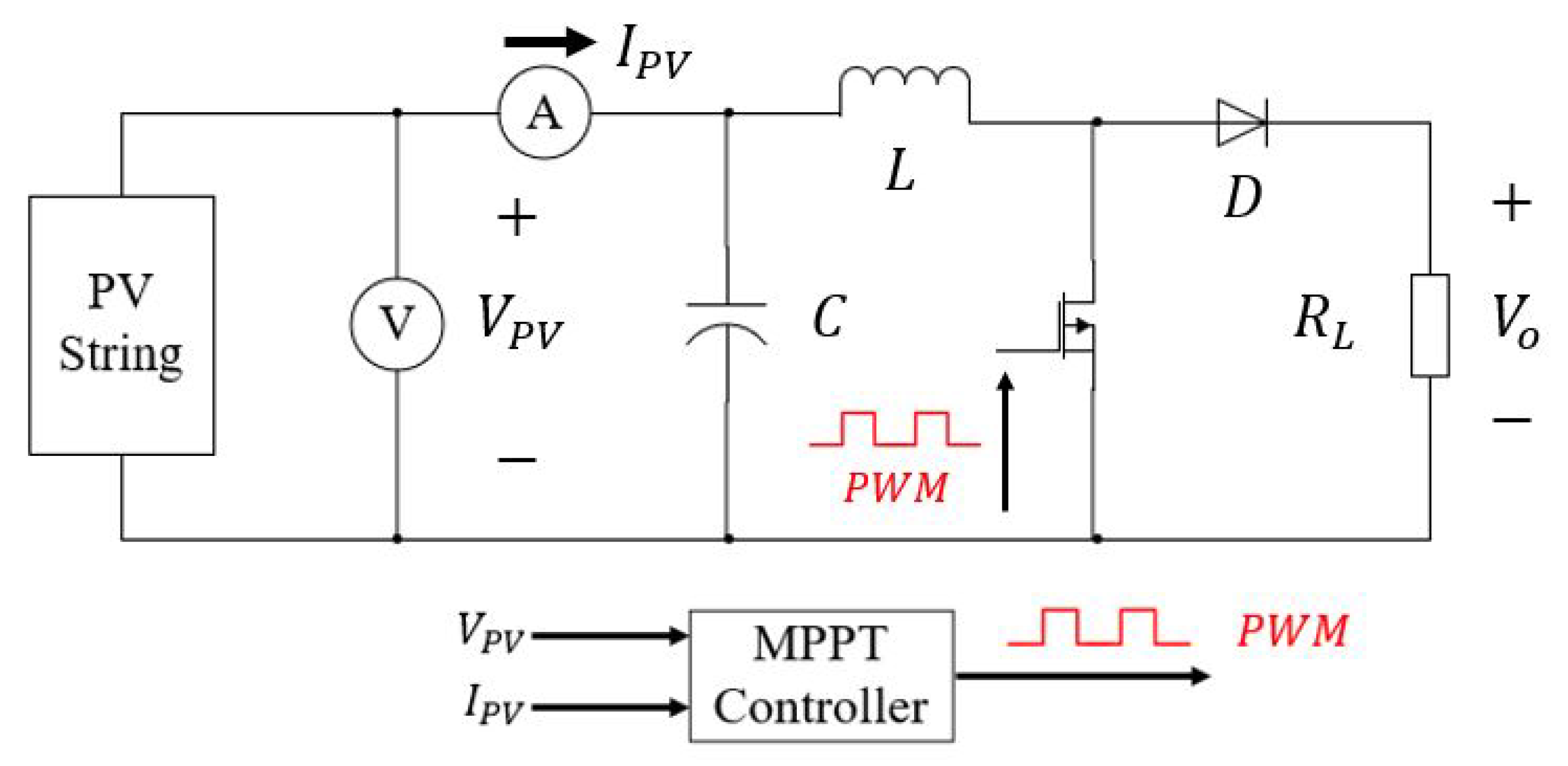
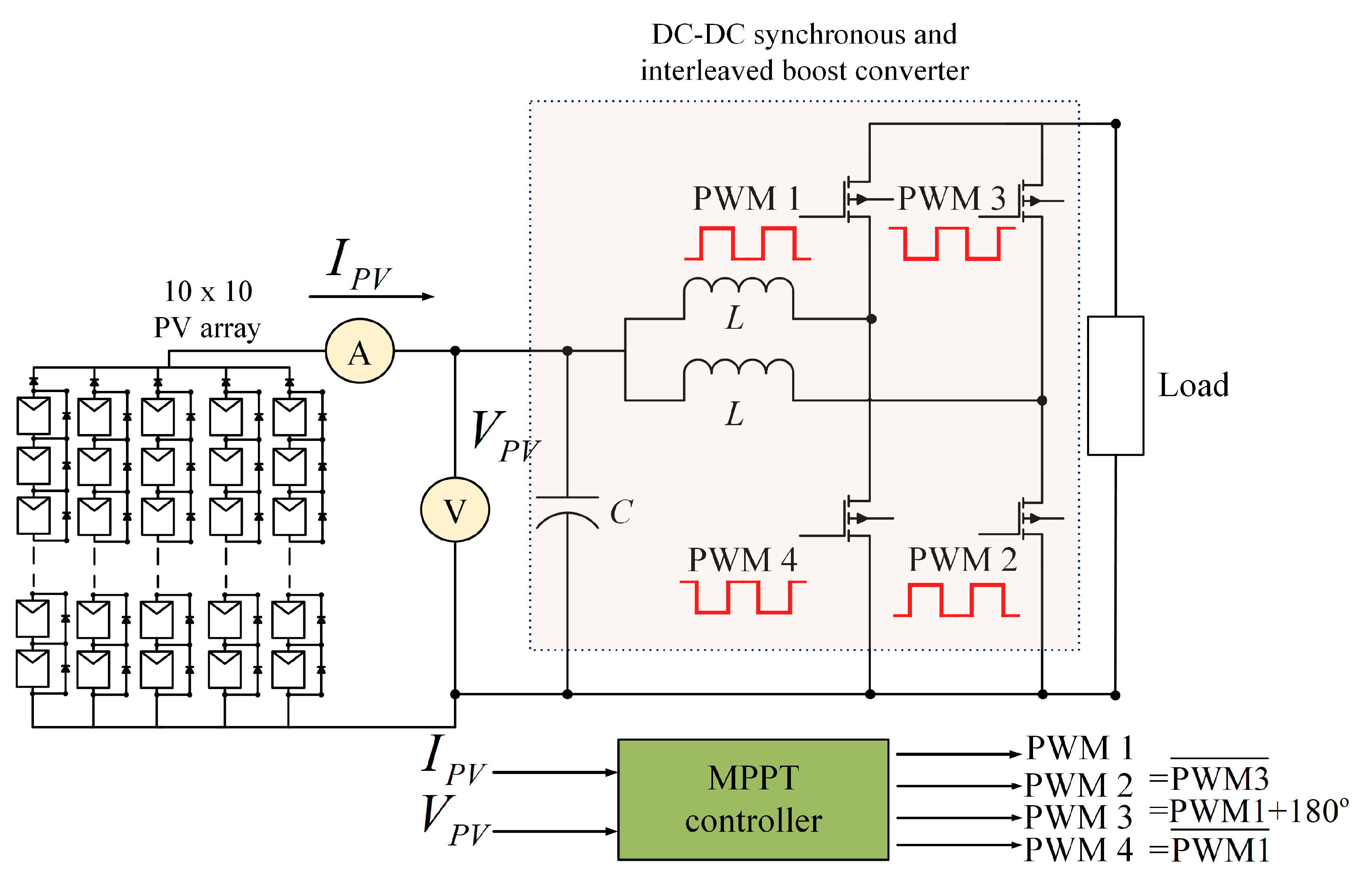
3.1. System Description

Generally, for the PV system, a DC-DC converter is implemented together with the MPPT controller to control the input voltage and current from PV to reach its maximum power point. In this case, it is assumed that the PV system connects to the constant DC load voltage. For this paper, the DC-DC boost converter is used to test the proposed method due to its robustness and simple switching control with only one duty cycle value (d). As for other converter topology (i.e., a buck-boost converter, single-ended primary-inductor converter (SEPIC)), the proposed algorithm can also be integrated; however, additional switching control is required since the number of switches adds and the converter operates in both buck and boost mode. Figure 5 shows the basic block diagram of the PV system integrated with the boost converter [41,42].
After measuring the PV’s voltage and current, the MPPT controller determines the maximum power point according to the level of irradiation and temperature. By tracking, the controller outputs the duty cycle to control the PV system to operate at its maximum power. Equation (3) demonstrates the mathematical relations between PV voltage V P V , load voltage V O , and duty cycle d.
V P V = ( 1 d ) V O
d is used to generate the pulse width modulation (PWM) switching signal to control the metal-oxide semiconductor field-effect transistor MOSFET. The challenge for this model is the accuracy. In order to achieve an accurate V P V , at maximum power, the tracking system is necessary.

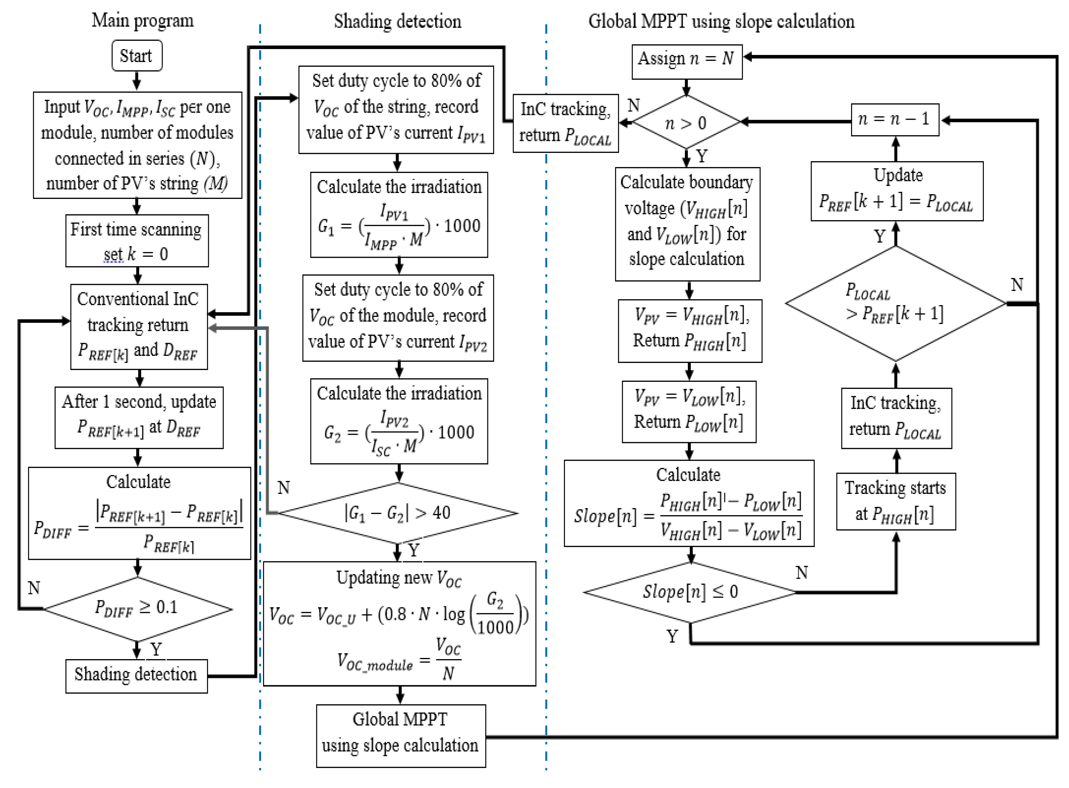
3.2. Proposed Global MPPT Algorithm

Figure 6 shows how the proposed global MPPT algorithm works. It mainly divides into three parts, which include the main program, shading detection, and global MPPT tracking using slope calculation, as presented.

3.2.1. Main Program

The first step is to input the necessary parameters of the PV module. These include a single PV module’s open-circuit voltage ( V O C ), short-circuit current ( I S C ), and PV current at maximum power point ( I M P P ) given from the manufacturer. Additionally, the number of modules connected in series (N) and the number of PV stings connected in the system (M) are inputted in the main program. When the program starts its operation, first time scanning is performed in order to determine the first maximum power point and maintains tracking with the conventional Incremental and conductance method (InC), where the tracked power is assigned as the reference point P R E F [ k ] at the duty cycle D R E F . The system keeps tracking at D R E F , and after one second, the value of the maximum power point is updated as P R E F [ k + 1 ] , which is the next sample. After this, the ratio of power changes, calculated as P D I F F , shown in Equation (4).
P D I F F = P R E F [ k + 1 ] P R E F [ k ] P R E F [ k ]
In order to identify if the value of P D I F F is suitable for starting global MPPT tracking, as mentioned by Ahmed [43], the threshold needs to be chosen. If the threshold is too large, MPPT cannot initiate global MPPT, but if too small, the algorithm could perform a false trigger with unnecessary global MPPT, leading to the wastage of tracking time and power.
In Reference [44], if the setup threshold is set to 15% of power change, this condition does not guarantee the detection for all shading cases. Moreover, for Reference [39], the threshold is set up to 5%. There is no evidence of how effective this value is, but in practice, it is considered to be too small. Referring to Yi-hwa [45] and Seyedmahnoudian [46], the studies use the standard formula’s review to set up a threshold. The threshold value of 0.1 (10%) is in popular use when assuming the average change of weather condition is assigned. In this case, as the weather in Tokyo, Japan does not change rapidly, the threshold of 0.1 is used. The algorithm calculates whether or not P D I F F exceeds the threshold. If it has exceeded it, the program enters the next function, which is shading detection, whereas when the change does not exceed the threshold, the program resumes standard InC tracking.

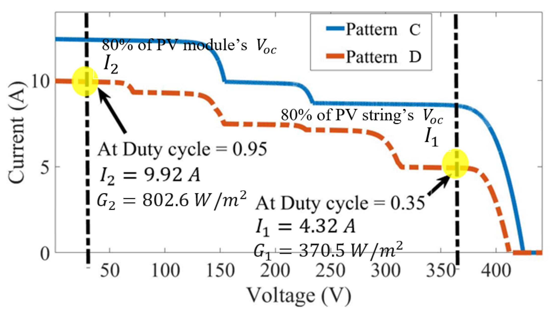
3.2.2. Shading Detection

The next section is shading detection. The primary purpose of this section is to determine whether the changes are due to partial shading or not. Even though change of power is detected, it is still unknown whether the changes have the trend of an increasing or decreasing power level. In this case, the irradiation is the critical parameter to determine the changes of power. According to other studies on solar irradiation estimation, there are several novel techniques of algorithm proposed. For example, in Reference [47], the paper presents a closed-form expression for solar irradiance with algebraic expression. The expression mainly estimated the irradiation as the function of temperature, PV current, and voltage. Although this method can estimate irradiation, the additional temperature sensor still needs to be installed, which increases the cost. This is in the same manner for Reference [48], which proposed the cloud motion estimation for short-term solar irradiation prediction. The method uses the motion vector of passing cloud with the previous irradiation monitoring data recorded before the estimation. For the proposed method, using the expression from Equation (1), assuming the change of temperature is not significant, the instantaneous irradiation can be estimated. Either the new temperature or irradiation sensors are not required and different from other novel topology; the irradiation data record is also not required. This makes the method simpler to implement.
According to Equation (1), the increase in PV current is the consequence of the irradiation. Starting from the calculation, the program calculates irradiation at the PV short-circuit current ( G 1 ) and at 80% of PV open-circuit voltage of PV string ( G 2 ) . By setting up the duty cycle, current I P V 1 and I P V 2 are measured and used to calculate irradiation. Equations (5) and (6) demonstrate how irradiation G 1 and G 2 is calculated. Using the ratio between PV measured current with I M P P and I S C , respectively, and multiplying with 1000, which is the irradiation at STC, the irradiation G 1 and G 2 can be obtained.
G 1 = I P V 1 I M P P · M · 1000
G 2 = I P V 2 I S C · M · 1000
After calculating the irradiation, the values are used to determine whether shading happens or not. According to Reference [43], the experiment is performed by testing samples of monocrystalline and polycrystalline PV panels and determining the threshold of difference between the irradiations. The testing achieves the threshold of 40. If the difference is greater than 40, it means partial shading can occur, more than one local power peaks exist, and the proposed global MPPT algorithm uses slope calculation calls.
G 1 G 2 | > 40
As shown in Equation (7), if the absolute difference between G 1 and G 2 is greater than 40, partial shading has a high possibility to occur. In this case, the value of PV open-circuit voltage ( V O C ) is updated (as presented in Equation (2) that V O C can change due to the impact from the temperature). In this case, the updated V O C can be calculated using Equation (8). The PV open-circuit voltage per one module ( V O C _ m o d u l e ) can also be estimated by dividing V O C with the input number of PV modules N.
V O C = V O C _ U + ( 0.8 · N · log ( G 2 1000 ) )
V O C _ m o d u l e = V O C N
According to Equations (8) and (9), V O C _ U is the PV open-circuit voltage at STC; using Equations (8) and (9), the values of PV open-circuit voltage can be updated. The new value of V O C contributes to more precise and accurate tracking for the proposed algorithm, which is explained in the following section. Additionally, the updated values are tested in short-term testing as part of the simulation result so that the efficiency can be confirmed.

3.2.3. Global MPPT Using Slope Calculation

The last section of the proposed algorithm is called “Global MPPT using slope calculation”, which was published in the authors’ published paper [49]. The concept of this algorithm is based on the inclined and declined slopes on each section of the P-V characteristic curve. The curve of the PV array is divided into sections based on the value of V O C _ m o d u l e from the main program part (or from the shading detection part if it has been updated). A step-by-step procedure of this section is described using the example in Section 3.2.4.

3.2.4. Example

The proposed system is tested by setting up 2 PV strings connected in parallel, each of which has 5 PV panels connected in series, as shown in Figure 7a,b. Patterns C and D are defined for different irradiation and temperature (25 °C and 30 °C, respectively). Table 2 presents the parameters for a single PV module used in this example. Based on the proposed algorithm in Figure 6, the algorithm starts to operate—the demonstration of the algorithm is present in Figure 8 and Figure 9 with the I-V and P-V curves. Firstly, first time scanning is performed for pattern C since it is the initialization of the process. The system found the global power peak (point 2 in Figure 9) and remained at the point using the conventional InC method. After 1 second, pattern D started to operate with less irradiation and more temperature. rising from 25 °C to 30 °C; the tracking point moved from point 2 to point 3 at the same duty cycle. the decrease of tracked power is recognized here, so the change of power detection algorithm operates. The system acknowledges the decrease, since the value of P D I F F calculated is 0.40 ( P D I F F = 1480 2472 2472 = 0.40 ), in this case, which is greater than 0.1; then, the system can detect the change of power.
Following the second part of the algorithm, which is the shading detection, the primary objective is to determine whether the detected change of power is caused by partial shading or not. Due to the fact that the change of power can also occur from the increase of irradiation (restored to the uniform irradiation at 1000 W / m 2 ), Global MPPT is considered to be unnecessary. In order to prevent additional tracking, the shading detection applies. The detection can be determined from the I-V characteristic curve, as shown in Figure 8.
In order to detect the shading, Equations (4) and (5) are used to calculate the irradiation G 1 and G 2 . The duty cycle is set to be 0.35 and the current I 1 is measured as 4.32 A. Using Equation (5), the irradiation G 1 is equal to 370.5 W / m 2 . Similarly for the duty cycle of 0.95, the current I 2 is measured given the value of 9.92, and the irradiation G 2 is 802.6 W / m 2 . The difference between G 1 and G 2 is calculated and compared with the threshold set in Equation (6). The difference is 370.50 802.60 | = 432.10 . which is higher than 40. From this result, the system considers the I-V characteristic curve as shaded. According to Section 3.2.2., the value of PV open-circuit voltage V O C is updated using Equation (8).
V O C = 428 + ( 0.8 · 5 · log 802.6 1000 ) = 427.12 V
V O C _ m o d u l e = 427.12 5 = 85.42 V
From the calculation result, V O C reduces due to the increase of the temperature. The updated value of V O C uses in the global MPPT’s part. After the system acknowledged that the shading occurs with more than one power peak located in the P-V characteristic curve, global MPPT uses a slope calculation, which is the final part the algorithm performs. Figure 9 shows the steps of how the proposed global maximum power point (GMPPT) operates.
The system starts to track from point 4, which is the rightmost region of the P-V curve and has the highest percentage of global power peak to be located. Since the number of PV panels connected in series is 5 ( N = 5 ) , the system calculates the reference point for calculating the slope, shown as dark blue and light blue points in Figure 9. The slope calculation points are assigned based on the test mentioned in the introduction. The analysis shows the MPP exists between 70–85% of the multiples of open-circuit voltage except for the two rightmost regions, which are the regions between 75–95%. According to this information, the slope calculation chooses from the multiples of each open-circuit voltage in the region deducted by the scaling ratio. Equations (10) and (11) show the calculation for each slope calculation point on the P-V curve.
V H I G H [ n ] = ( V O C _ m o d u l e · n ) [ ( 1 0.46 ) · V O C _ m o d u l e ] , n > N 2 ( V O C _ m o d u l e · n ) [ ( 1 0.51 ) · V O C _ m o d u l e ] , o t h e r w i s e
V L O W [ n ] = ( V O C _ m o d u l e · n ) [ ( 1 0.51 ) · V O C _ m o d u l e ] , n > N 2 ( V O C _ m o d u l e · n ) [ ( 1 0.56 ) · V O C _ m o d u l e ] , o t h e r w i s e
where N is the number of the PV module connected in series, and n is the variable assigned in the flowchart in Figure 6. Using Equations (10) and (11), all slope calculation points can be calculated. For example, the rightmost blue point is assigned as V H I G H [ 5 ] , which is calculated from Equation (10) as:
V H I G H [ 5 ] = ( V O C _ m o d u l e · 5 ) [ ( 1 0.46 ) · V O C _ m o d u l e ] = ( 85.42 · 5 ) [ ( 1 0.46 ) · 85.42 ] = 381.54 V
.
The PV voltage is controlled by the duty cycle to move to the point; after that, the reference power ( P H I G H [ 5 ] ) is measured as 8.21 W. Following the next reference point V L O W [ 5 ] determined from Equation (11):
V L O W [ 5 ] = ( V O C _ m o d u l e · 5 ) [ ( 1 0.51 ) · V O C _ m o d u l e ] = ( 85.42 · 5 ) [ ( 1 0.51 ) · 85.42 ] = 385.6 V
.
In the same manner, the reference power ( P L O W [ 5 ] ) is recorded as 3.45 W. The system then uses this information to calculate the slope at the rightmost region.
S l o p e [ 5 ] = P H I G H [ 5 ] P L O W [ 5 ] V H I G H [ 5 ] V L O W [ 5 ] = 8.21 3.45 381.54 385.6 = 1.17
From the calculation, the negative value of the slope is shown, so the graph has a trend of incline, and the power peak can exist. Because of this, the system starts the conventional tracking at the region using InC and finds point 5 as the local power peak. The value is assigned as P L O C A L and saved for comparison with tracked powers in other regions. The steps are repeated in other regions of the P-V characteristic curves from regions 4 to 1. For this part, V H I G H [ n ] and V L O W [ n ] are tracked in each region. Table 3 presents the summarized result of the slope calculation in each region of the P-V curve. The system finds the power peak in regions 4 and 2 but finds the decline slope in regions 3 and 1 according to Figure 9.
From the results shown in Table 3, the proposed algorithm locates the global power peak in region 4 (1710.00 W). The result confirmed by Figure 9 shows where the maximum power point is located. Overall, this example demonstrates the operations of the proposed algorithm step by step and verifies the result of MPPT.

4. Simulation Results

In order to test the performance of the proposed Global MPPT algorithm, short-term and long-term testing are performed. Figure 10 shows the circuit diagram of how the proposed global MPPT is tested. The circuit consists of PV arrays (ten strings with ten panels connected in series), where each panel has the specification as described in Table 2, with voltage and current sensors and a DC-DC converter circuit, which is the synchronous and interleaved boost converter. The working principle is similar to the two-phase DC-AC converter when switches on the opposite legs will synchronously turn on. As labelled in Figure 10, for the period T s , switches 1 and 2 will turn on, while switches 3 and 4 will be turned off. In sequence, for the next period ( 1 T s ) , switches 1 and 2 will be turned off instead, while switched 3 and 4 will be on. Voltages can be determined using the boost converter mathematical expression from Equation (3).

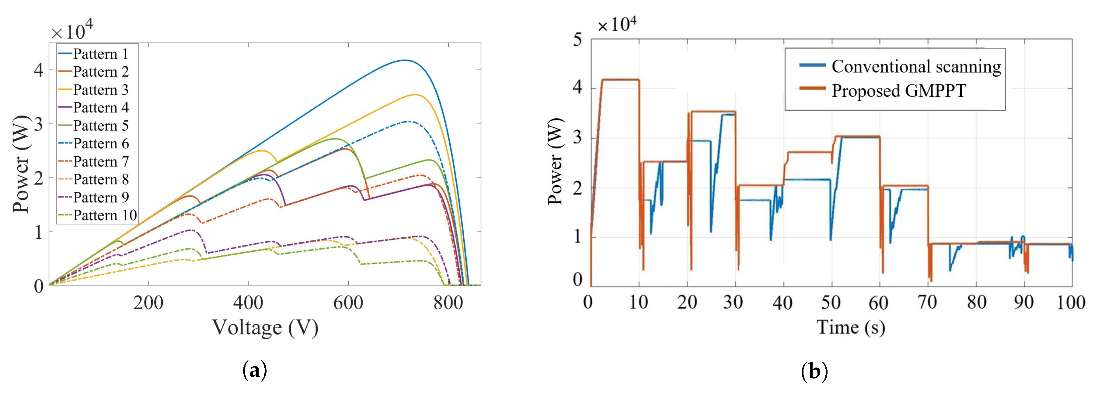
4.1. Short-Term Testing

For short-term testing, case studies of ten different P-V characteristic curves are used to test the proposed algorithm. Using P-V characteristic curves from patterns 1 to 10, as shown in Figure 11a and applied to the circuit in Figure 10, graphical and numerical results are considered. Each pattern is set to change to the next pattern at ten-second intervals. Figure 11b presents the graphical results of power tracking using the proposed algorithm compared to conventional scanning.
Table 4 presents the performance comparison of conventional scanning and the proposed GMPPT algorithm. It can be observed that the tracking time used for the proposed global MPPT method is less than the conventional scanning method. This reduces tracking time and consumes less power during the tracking operation. The loss of power gradually reduces each time tracking is performed.

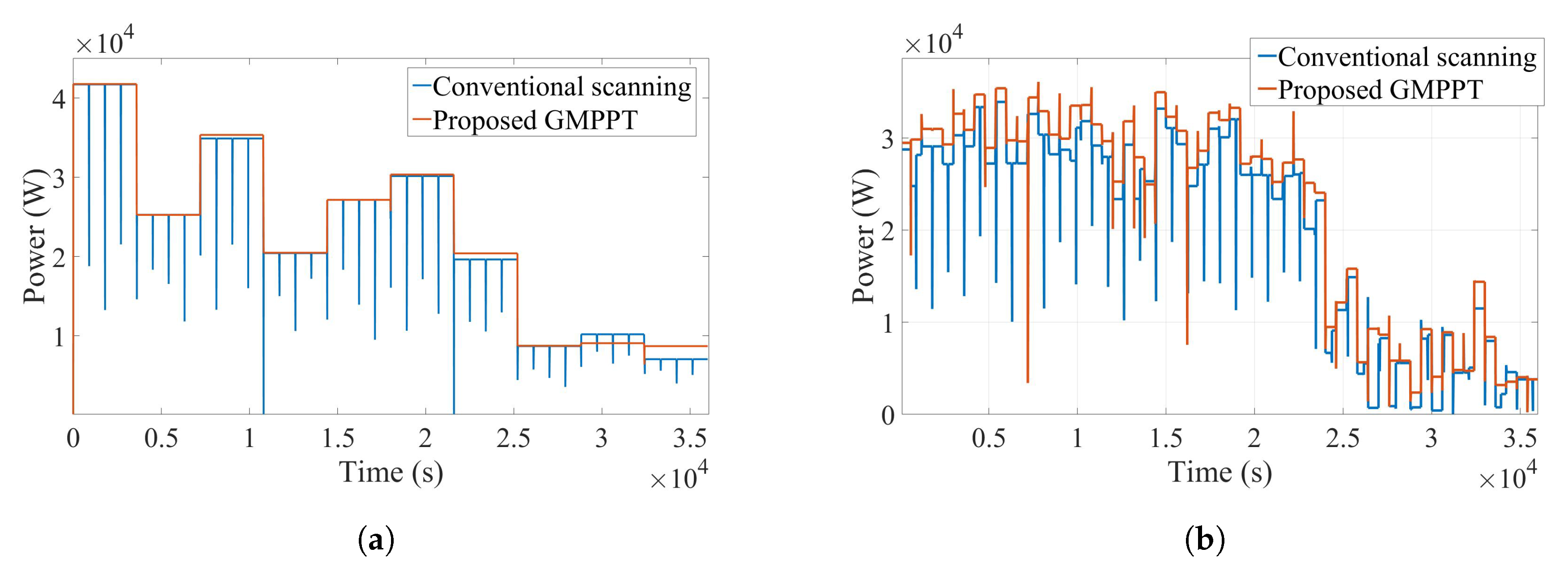
4.2. Long-term Testing

In order to perform the testing as demonstrated in the daytime operation similar to what the PV system operates in one day, the long-term test simulates different weather conditions in a period of 10 h (36,000 s). The test divides into a steady and rapid change of weather conditions, in which the information is collected from the real measured data at Shibaura Institute of Technology, Tokyo, Japan in June 2018. Figure 12a,b shows the graphical results of tracking power using the scanning and proposed algorithm. The scanning is set to be as default every 15 min, as described in the introduction.
Table 5 presents the numerical results for long-term testing. Results show the total power achieved per day, per annum, and estimated revenue achieved using an energy selling rate in Tokyo, Japan in 2018 (20 JPY per kWh).
This shows the proposed GMPPT can increase revenue and have more additional income compared to the conventional scanning method, which creates benefits in the operating day. Additionally, for the rapid change condition, the proposed method can enhance the total energy of 8.55% compared to the conventional algorithm. As described from short-term testing, the advantage of the proposed algorithm is not only the performance to operate in both steady and rapid change weather conditions; the tracking speed enhancement also reduces power loss. To summarize, the tracking speed enhancement is shown in the short-term testing, where each track has less power loss than conventional scanning. Consequently, it increases the energy generated from the PV system when operated in long-term.

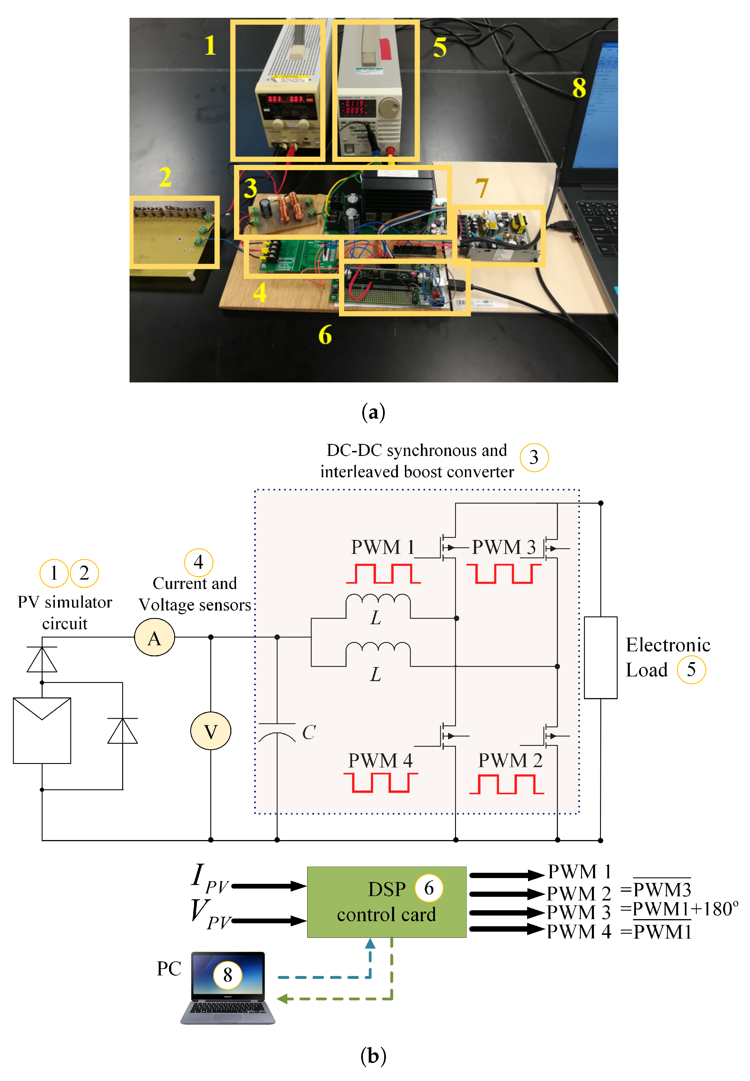
5. Experimental Results

For the experiment, the primary circuit system used is the synchronous and interleaved DC-DC boost converter shown in Figure 13a. The MPPT algorithm is programmed using a Texas instrument F28335 digital signal processor (DSP) control card where the input voltage and current is inputted via the sensor unit to scale down the parameters before inputting to the control card. The PWM signals (PWM 1 to 4) are generated and sent to the switches. Figure 13a shows the photo of the experiment system; the list of the components includes (1) a DC power supply, (2) a PV simulator circuit, (3) a DC-DC synchronous and interleaved boost converter, (4) a voltage and current sensor, (5) electronic load, (6) a DSP control card, (7) 12V DC power supply and (8) a laptop for data acquisition. The switching control of this converter is performed by setting up the phase shift, according to Figure 13b. The inverted switching waveform consists of PWM4 (inverted from PWM1) and PWM2 (inverted from PWM3); the phase shift is set to be fixed at 180° for PWM3 (shifted from PWM1 which is the primary signal).
The test consists of two different short-circuit current values set using the DC power supply to represent the different irradiation. The current is set as 1.03 A for level I of irradiation and 0.89 A for level II. The programs have a task to track the power changed from level I to II before restoring to level I again. The setup parameters for the experiment included the sampling frequency as 10 kHz for the scanning and proposed method, and the incremental step is 0.2 s, which is the minimum step in which the tested DC-DC converter can operate efficiently. The experimental results are achieved from the voltage and current sensors connected to the converter’s circuit, then evaluated in the control card and imported to the PC. Figure 14a,b shows the graphical results of tracking.
From the result shown in Figure 14a, the conventional scanning takes approximately 4.96 s to track the power from level I to level II, which gives the value of 16.3 W and 12.6 W, respectively. As for the proposed method in Figure 14b, it takes approximately 0.42 s The result confirms the simulation outcome that scanning consumes more time to scan throughout all values of power. The experiment verifies the performance of both algorithms.

6. Conclusions

This research proposes the studies of P-V characteristic curves, partial shading detection, and a global maximum power point tracking algorithm. As irradiation and temperature affect generated power, the work presents an analysis using mathematical equations. The simulation result shows the tracking process is successful, with accuracy and requiring less tracking time compared to conventional scanning. More energy is achieved by 8.55% from the long-term study, which also increases revenue. The experimental result shows successful tracking when the change of irradiation happens. This paper’s proposed algorithm is advantageous because it requires fewer samples and less power loss, while tracking increases the energy achieved.

Author Contributions

J.G. conceived the methodology, developed the theory, performed the computations, and prepared this paper. G.F. performed the supervision, provided critical feedback, and helped to shape the research.

Funding

This research received no external funding.

Acknowledgments

The authors would like acknowledge the assistance of two researchers and a student from Shibaura Institute of Technology. Firstly, thanks to Duy-Dinh Nguyen for the technical support. Secondly, thanks to Kawabata Machiya for providing the weather information data used in this research.

Conflicts of Interest

The authors declare no conflict of interest.

Abbreviations

The following abbreviations are used in this manuscript:
ANNArtificial neural network
dDuty cycle
DSPDigital signal processor
GIrradiation
GMPPTGlobal maximum power point tracking
I-VCurrent–voltage
InCIncremental conductance
JPYJapanese Yen
MDPIMultidisciplinary Digital Publishing Institute
MOSFETMetal-Oxide Semiconductor Field-Effect Transistor
MPPMaximum power point
MPPTMaximum power point tracking
P&OPerturb and pbserve
P-VPower–voltage
PSOParticle swarm pptimization
PVPhotovoltaic
PWMPulse width modulation
SEPICSingle-ended primary-inductor converter
STCStandard test conditions
TTemperature

References

  1. Romero-Cadaval, E.; Spagnuolo, G.; Franquelo, L.G.; Ramos-Paja, C.A.; Suntio, T.; Xiao, W.M. Grid-Connected Photovoltaic Generation Plants: Components and Operation. IEEE Ind. Electron. Mag. 2013, 7, 6–20. [Google Scholar] [CrossRef] [Green Version]
  2. Patel, H.; Agarwal, V. MATLAB-Based Modeling to Study the Effects of Partial Shading on PV Array Characteristics. IEEE Trans. Energy Convers. 2008, 23, 302–310. [Google Scholar] [CrossRef]
  3. Femia, N.; Lisi, G.; Petrone, G.; Spagnuolo, G.; Vitelli, M. Distributed maximum power point tracking of photovoltaic arrays: Novel approach and system analysis. IEEE Trans. Ind. Electron. 2008, 55, 2610–2621. [Google Scholar] [CrossRef] [Green Version]
  4. Gao, L.; Dougal, R.A.; Liu, S.; Iotova, A.P. Parallel-Connected Solar PV System to Address Partial and Rapidly Fluctuating Shadow Conditions. IEEE Trans. Ind. Electron. 2009, 56, 1548–1556. [Google Scholar] [Green Version]
  5. Eftichios, K. A New Technique for Tracking the Global Maximum Power Point of PV Arrays Operating Under Partial-Shading Conditions. IEEE J. Photovolt. 2012, 2, 184–190. [Google Scholar] [Green Version]
  6. Daraban, S.; Petreus, D.; Morel, C.; Machmoum, M. A novel global MPPT algorithm for distributed MPPT systems. In Proceedings of the 15th European Conference on Power Electronics and Applications (EPE), Lille, France, 2–6 September 2013; pp. 1–10. [Google Scholar]
  7. Pillai, D.S.; Rajasekar, N. A comprehensive review on protection challenges and fault diagnosis in PV systems. Renew. Sustain. Energy Rev. 2018, 18–40. [Google Scholar] [CrossRef]
  8. Veerachary, M. PSIM circuit-oriented simulator model for the nonlinear photovoltaic sources. IEEE Trans. Aerosp. Electron. Syst. 2006, 42, 735–740. [Google Scholar] [CrossRef]
  9. Tey, K.S.; Mekhilef, S. Modified Incremental Conductance Algorithm for Photovoltaic System Under Partial Shading Conditions and Load Variation. IEEE Trans. Ind. Electron. 2014, 61, 5384–5392. [Google Scholar]
  10. Ji, Y.; Jung, D.; Won, C.; Lee, B.; Kim, J. Maximum power point tracking method for PV array under partially shaded condition. In Proceedings of the IEEE Energy Conversion Congress and Exposition, San Jose, CA, USA, 20–24 September 2009; pp. 307–312. [Google Scholar]
  11. Sera, D.; Mathe, L.; Kerekes, T.; Spataru, S.V.; Teodorescu, R. On the Perturb-and-Observe and Incremental Conductance MPPT Methods for PV Systems. IEEE J. Photovolt. 2013, 3, 1070–1078. [Google Scholar] [CrossRef]
  12. Nguyen, T.L.; Low, K. A Global Maximum Power Point Tracking Scheme Employing DIRECT Search Algorithm for Photovoltaic Systems. IIEEE Trans. Ind. Electron. 2010, 57, 3456–3467. [Google Scholar] [CrossRef]
  13. Malik, S. MPPT Schemes for PV System under Normal and Partial Shading Condition: A Review. Int. J. Renew. Energy Dev. 2016, 2, 79–94. [Google Scholar]
  14. Alik, R.; Jusoh, A.; Shukri, N.A. An improved perturb and observe checking algorithm MPPT for photovoltaic system under partial shading condition. In Proceedings of the IEEE Conference on Energy Conversion (CENCON), Johor Bahru, Malaysia, 19–20 October 2015. [Google Scholar]
  15. Kapić, A.; Zečević, Ž.; Krstajić, B. An efficient MPPT algorithm for PV modules under partial shading and sudden change in irradiance. In Proceedings of the 23rd International Scientific-Professional Conference on Information Technology (IT), Zabljak, Montenegro, 19–24 February 2018. [Google Scholar]
  16. Duan, Q.; Leng, J.; Duan, P.; Hu, B.; Mao, M. An Improved Variable Step PO and Global Scanning MPPT Method for PV Systems under Partial Shading Condition. In Proceedings of the 7th International Conference on Intelligent Human-Machine Systems and Cybernetics, Hangzhou, China, 26–27 August 2015. [Google Scholar]
  17. Başoğlu, M.E.; Çakir, B. Experimental evaluations of global maximum power point tracking approaches in partial shading conditions. In Proceedings of the 2017 IEEE International Conference on Environment and Electrical Engineering and 2017 IEEE Industrial and Commercial Power Systems Europe (EEEIC/I&CPS Europe), Milan, Italy, 6–9 June 2017. [Google Scholar]
  18. Bidyadhar, S. A Comparative Study on Maximum Power Point Tracking Techniques for Photovoltaic Power Systems. IEEE Trans. Sustain. Energy 2013, 4, 89–97. [Google Scholar]
  19. Kinattigal, S. Enhanced Energy Output From a PV System Under Partial Shading Conditions through Artifical Bee Colony. IEEE Trans. Sustain. Energy 2015, 6, 198–209. [Google Scholar]
  20. Hiren, P. Maximum Power Point Tracking Scheme for PV Systems Operating under Partially Shaded Conditions. IEEE Trans. Ind. Electron. 2008, 55, 1689–1698. [Google Scholar]
  21. Jubaer, A. An Enhanced Adaptive P&O MPPT for Fast and Efficient Tracking under Varying Environment. IEEE Trans. Ind. Electron. 2008, 55, 1689–1698. [Google Scholar]
  22. Korey Sener, P. A New MPPT Method for PV Array System under Partially Shaded Conditions. In Proceedings of the 3rd International Symposium on Power Electronics for Distributed Generation Systems (PEDG), Aalborg, Denmark, 25–28 June 2012; pp. 437–441. [Google Scholar]
  23. Kobayashi, K.; Takano, I.; Sawada, Y. A study on a two stage maximum power point tracking control of a photovoltaic system under partially shaded insolation conditions. In Proceedings of the IEEE Power Engineering Society General Meeting (IEEE Cat. No. 03CH37491), Toronto, ON, Canada, 13–17 July 2003; pp. 2612–2617. [Google Scholar]
  24. Irisawa, K.; Saito, T.; Takano, I.; Sawada, Y. Maximum power point tracking control of photovoltaic generation system under non-uniform insolation by means of monitoring cells. In Proceedings of the Conference Record of the Twenty-Eighth IEEE Photovoltaic Specialists Conference, Anchorage, AK, USA, 15–22 September 2000; pp. 1707–1710. [Google Scholar]
  25. Bekker, B.; Beukes, H.J. Finding an optimal PV panel maximum power point tracking method. In Proceedings of the 2004 IEEE Africon 7th Africon Conference in Africa, Gaborone, Botswana, 15–17 September 2004; pp. 1125–1129. [Google Scholar]
  26. Nguyen, D.; Lehman, B. An Adaptive Solar Photovoltaic Array Using Model-Based Reconfiguration Algorithm. IEEE Trans. Ind. Electron. 2008, 2644–2654. [Google Scholar] [CrossRef]
  27. Gules, R.; Pacheco, J.D.P.; Hey, H.L.; Imhoff, J. A Maximum Power Point Tracking System with Parallel Connection for PV Stand-Alone Applications. IEEE Trans. Ind. Electron. 2008, 55, 2674–2683. [Google Scholar] [CrossRef]
  28. Uno, M.; Kukita, A. Current sensorless single-switch voltage equalizer using multi-stacked buck-boost converters for photovoltaic modules under partial shading. In Proceedings of the 9th International Conference on Power Electronics and ECCE Asia (ICPE-ECCE Asia), Seoul, Korea, 1–5 June 2015; pp. 645–651. [Google Scholar]
  29. Yuan, X.; Yang, D.; Liu, H. MPPT of PV system under partial shading condition based on adaptive inertia weight particle swarm optimization algorithm. In Proceedings of the IEEE International Conference on Cyber Technology in Automation, Control, and Intelligent Systems (CYBER), Shenyang, China, 8–12 June 2015. [Google Scholar]
  30. Miyatake, M.; Veerachary, M.; Toriumi, F.; Fujii, N.; Ko, H. Maximum Power Point Tracking of Multiple Photovoltaic Arrays: A PSO Approach. IEEE Trans. Aerosp. Electron. Syst. 2011, 47, 367–380. [Google Scholar] [CrossRef]
  31. Ishaque, K.; Salam, Z. A Deterministic Particle Swarm Optimization Maximum Power Point Tracker for Photovoltaic System under Partial Shading Condition. IEEE Trans. Ind. Electron. 2013, 60, 3195–3206. [Google Scholar] [CrossRef]
  32. Ishaque, K.; Salam, Z.; Amjad, M.; Mekhilef, S. An Improved Particle Swarm Optimization (PSO)—Based MPPT for PV with Reduced Steady-State Oscillation. IEEE Trans. Power Electron. 2012, 27, 3627–3638. [Google Scholar] [CrossRef]
  33. Alajmi, B.N.; Ahmed, K.H.; Finney, S.J.; Williams, B.W. A Maximum Power Point Tracking Technique for Partially Shaded Photovoltaic Systems in Microgrids. IEEE Trans. Ind. Electron. 2013, 60, 1596–1606. [Google Scholar] [CrossRef]
  34. ABB. ABB UNO PVI-3.0-3.6-3.8-4.2-TL-OUTD-S-US (-A) Product Manual. ABB Sol. Invert. 2016. Available online: https://library.e.abb.com/public/5c56393f1c9c734185257cda007edfe3/PVI-3.0-3.6-3.8-4.2-TL-OUTD-S-US%20(-A)%20Product%20manual.pdf (accessed on 12 October 2018).
  35. SMA, Sunny Boy 3000TL/3600TL/4000TL/5000TL Product manual. SMA Sol. Invert. 2016. Available online: http://files.sma.de/dl/15330/SB30-50TL-21-BE-en-11.pdf (accessed on 12 October 2018).
  36. Lyden, S.; Haque, M.E.; Gargoom, A.; Negnevitsky, M. Review of Maximum Power Point Tracking approaches suitable for PV systems under Partial Shading Conditions. In Proceedings of the Australasian Universities Power Engineering Conference (AUPEC), Hobart, Australia, 29 September–3 October 2013; pp. 1–6. [Google Scholar]
  37. Bastidas-Rodriguez, J.D.; Franco, E.; Petrone, G.; Ramos-Paja, C.A.; Spagnuolo, G. Maximum power point tracking architectures for photovoltaic systems in mismatching conditions: A review. IET Power Electron. 2014, 7, 1396–1413. [Google Scholar] [CrossRef]
  38. Karim, D. Backstepping sliding mode control for maximum power point tracking of a photovoltaic system. Electr. Power Syst. Res. 2017, 143, 182–188. [Google Scholar]
  39. Alireza, R. Global Maximum Power Point Tracking Method for Photovoltaic Arrays under Partial Shading Conditions. IEEE Trans. Ind. Electron. 2017, 64, 2855–2864. [Google Scholar]
  40. Moballegh, S.; Jiang, J. Modeling, Prediction, and Experimental Validations of Power Peaks of PV Arrays under Partial Shading Conditions. IEEE Trans. Sustain. Energy 2014, 5, 293–300. [Google Scholar] [CrossRef]
  41. Mohammad Amin, G. Partial Shading Detection and Smooth Maximum Power Point Tracking of PV Arrays under PSC. IEEE Trans. Power Electron. 2016, 31, 6281–6292. [Google Scholar]
  42. Wang, Y. High-Accuracy and Fast-Speed MPPT Methods for PV String under Partially Shaded Conditions. IEEE Trans. Ind. Electron. 2016, 63, 235–245. [Google Scholar] [CrossRef]
  43. Ahmed, J. An accurate method for MPPT algorithm to detect the Partial shading Occurrence in a PV system. IEEE Trans. Ind. Inform. 2017, 13, 2151–2161. [Google Scholar] [CrossRef]
  44. Kim, R.-Y. An improved global maximum power point tracking scheme under partial shading conditions. J. Int. Conf. Electr. Mach. Syst. 2013, 2, 65–68. [Google Scholar] [CrossRef]
  45. Yi-Hwa, L. A particle swarm optimization-based maximum power point tracking algorithm for PV systems operating under partially shaded conditions. IEEE Trans. Energy Convers. 2012, 27, 1027–1035. [Google Scholar]
  46. Seyedmahmoudian, M. Simulation and hardware implementation of new maximum power point tracking technique for partially shaded PV system using hybrid DEPSO method. IEEE Trans. Sustain. Energy 2015, 6, 850–862. [Google Scholar] [CrossRef]
  47. Carrasco, M.; Laudani, A.; Lozito, G.M.; Mancilla-David, F.; Riganti Fulginei, F.; Salvini, A. Low-Cost Solar Irradiance Sensing for PV Systems. Energies 2017, 10, 998. [Google Scholar] [CrossRef]
  48. Huang, H.; Xu, J.; Peng, Z.; Yoo, S.; Yu, D.; Huang, D.; Qin, H. Cloud motion estimation for short term solar irradiation prediction. In Proceedings of the 2013 IEEE International Conference on Smart Grid Communications (SmartGridComm), Vancouver, BC, Canada, 21–24 October 2013. [Google Scholar]
  49. Gosumbonggot, J.; Nguyen, D.D.; Fujita, G. Partial Shading and Global Maximum Power Point Detection Enhancing MPPT for Photovoltaic Systems Operated in Shading Condition. In Proceedings of the 53rd International Universities Power Engineering Conference (UPEC), Glasgow City, UK, 4–7 September 2018. [Google Scholar]
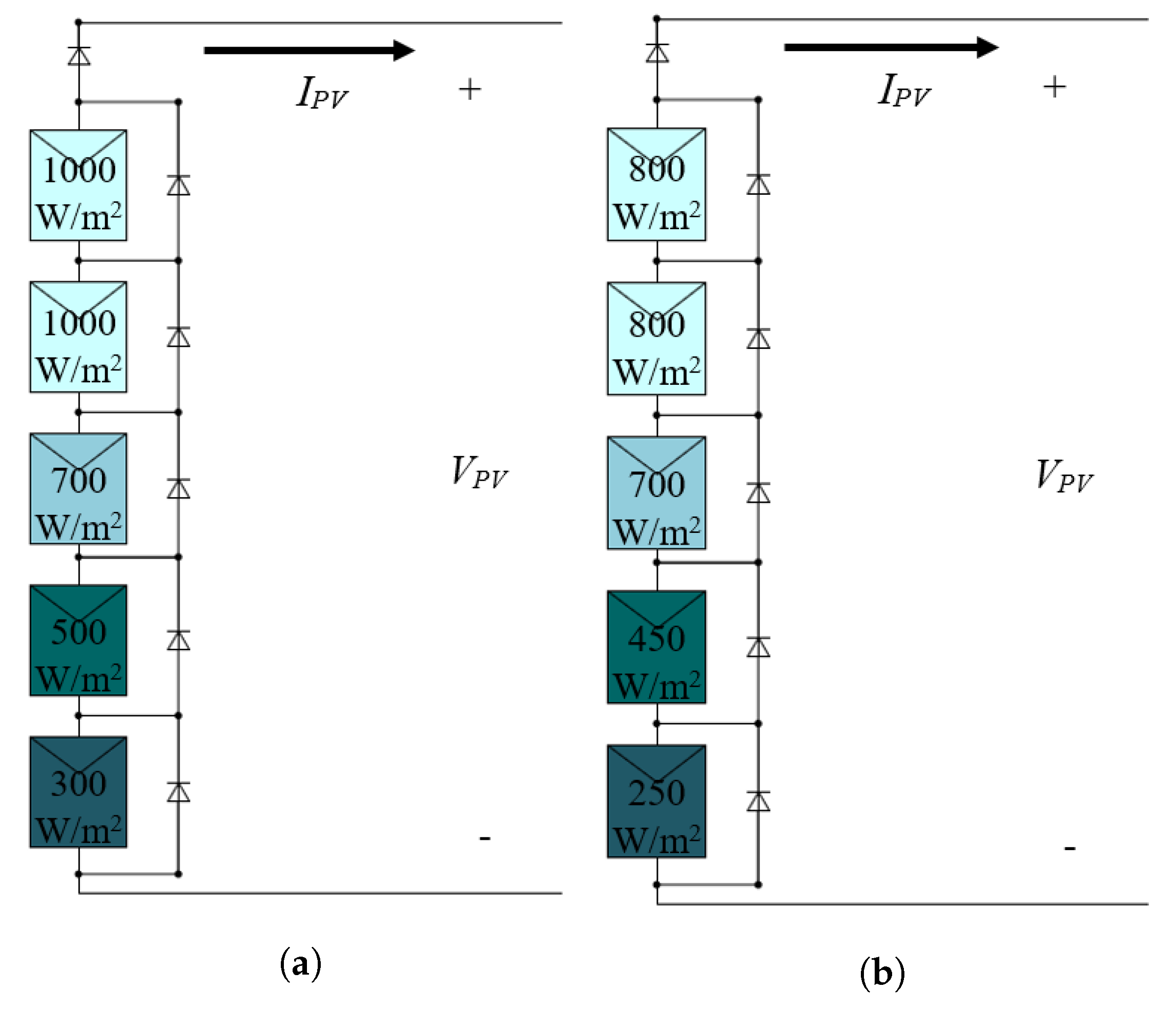
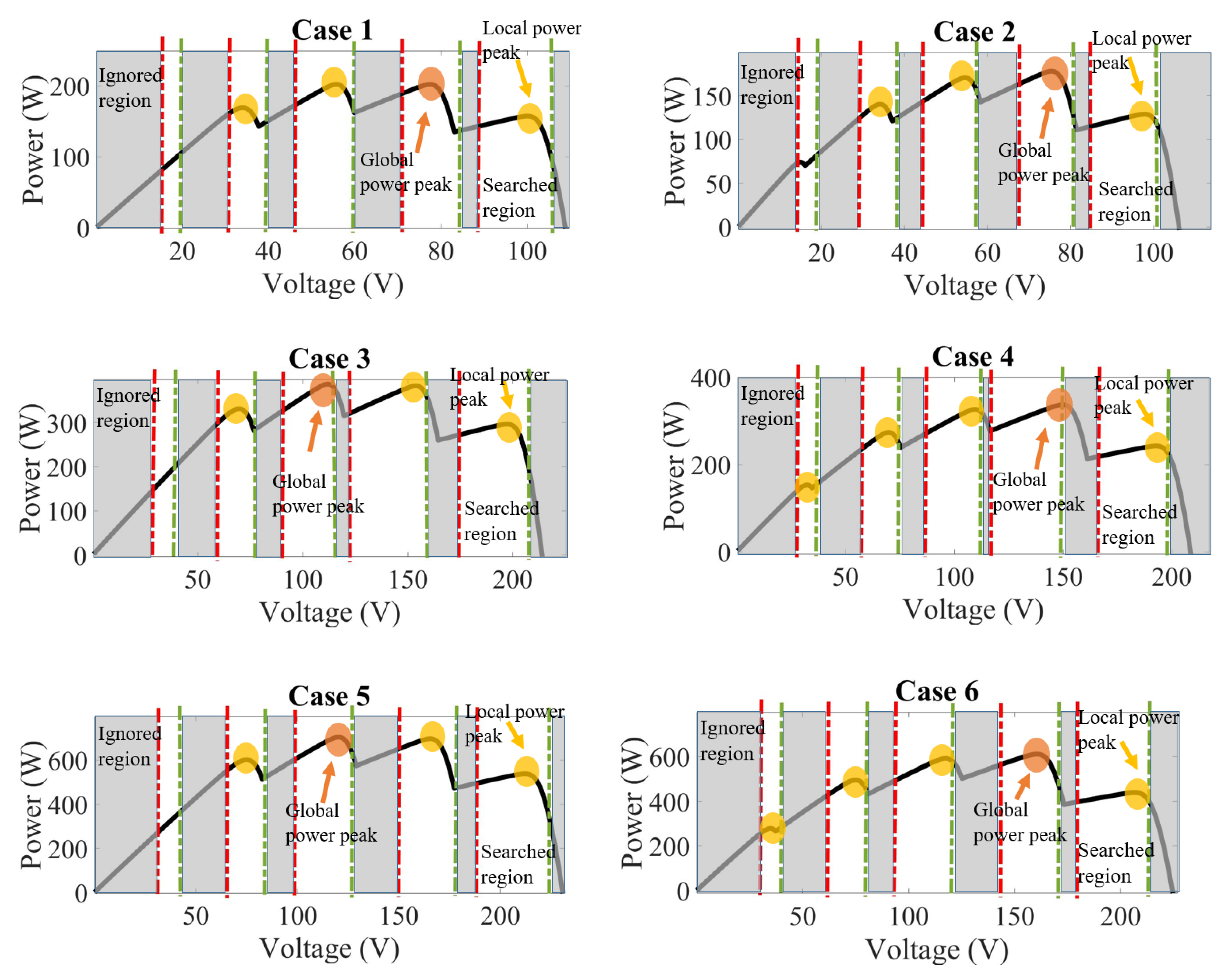
Figure 1. (a) Normal condition at 25 °C, (b) partial shading condition at 25 °C, (c) power-voltage (P-V) characteristic curves for both conditions.
Energies 12 00202 g001
Figure 2. Photovoltaic (PV) module equivalent circuit.
Energies 12 00202 g002
Figure 3. (a) Pattern A at 25 °C, (b) pattern B at 30 °C.
Energies 12 00202 g003
Figure 4. P-V characteristic curves for Cases 1–6.
Energies 12 00202 g004
Figure 5. Basic PV system with the DC-DC boost converter.
Energies 12 00202 g005
Figure 6. Flowchart of proposed global maximum power point tracking method (MPPT) algorithm.
Energies 12 00202 g006
Figure 7. (a) Pattern C at 25 °C, (b) pattern D at 30 °C.
Energies 12 00202 g007
Figure 8. Example current-voltage (I-V) characteristic curves for patterns C and D.
Energies 12 00202 g008
Figure 9. Example of P-V characteristic curves for patterns C and D.
Energies 12 00202 g009
Figure 10. System diagram for MPPT testing.
Energies 12 00202 g010
Figure 11. Short-term testing. (a) P-V characteristic curves for short-term testing; (b) result of tracked power.
Energies 12 00202 g011
Figure 12. Tracking power for long-term testing at tested weather conditions. (a) Steady change; (b) rapid change.
Energies 12 00202 g012
Figure 13. (a) Photograph of the experimental system. (b) Diagram of the experimental system.
Energies 12 00202 g013
Figure 14. Experimental results. (a) Conventional scanning; (b) proposed GMPPT algorithm.
Energies 12 00202 g014
Table 1. Summarized information of example cases.
CasePV Module’s SpecificationIrradiation Pattern V OC per Module ( V )
Case 1Canadian Solar Cs5C-90MA22.20
Case 2B21.24
Case 3Trina Solar TSM-170DA43.60
Case 4B41.72
Case 5Jinko Solar JKM310M-72A47.10
Case 6B44.90
Table 2. Parameters for Single PV module.
ParametersValue
Maximum power425 W
Current at maximum power5.83 A
Voltage at maximum power72.9 V
Short-circuit current6.18 A
Open-circuit voltage85.6 V
Voltage Temperature coefficient−0.36099 (%/°C)
Current Temperature coefficient0.102 (%/°C)
Table 3. Summarized result for Global MPPT using slope calculation of pattern C and D.
Region ( N ) Reference DataSlopeDecisionPower Tracked ( W )
P HIGH ( W ) V HIGH ( V ) P LOW ( W ) V LOW ( V )
1527.6943.56568.2047.839.48Not detected-
21220.00128.981230.00138.001.11Not detected-
31570.00215.121560.00219.18−1.96Detected1570.00
41700.00296.301680.00300.36−5.37Detected1710.00
58.21381.543.45385.60−1.17Detected1640.20
Table 4. Performance comparison of conventional scanning and proposed GMPPT algorithm using short-term testing.
Shading PatternTracking MethodPower ( W ) Tracking Speed ( s ) Maximum Power from P-V Curve ( W ) Efficiency (%)
1Conventional scanning41.672.3541.7599.81
Proposed GMPPT41.722.3399.93
2Conventional scanning25.242.4925.2699.92
Proposed GMPPT25.250.9199.96
3Conventional scanning34.712.5735.3698.16
Proposed GMPPT35.330.8799.92
4Conventional scanning17.422.0620.4885.06
Proposed GMPPT20.470.7199.95
5Conventional scanning21.612.7927.1479.62
Proposed GMPPT27.120.9199.93
6Conventional scanning30.102.4130.3799.11
Proposed GMPPT30.340.7799.90
7Conventional scanning19.633.3920.3996.27
Proposed GMPPT20.380.5699.95
8Conventional scanning8.872.658.9099.66
Proposed GMPPT8.730.7498.09
9Conventional scanning10.172.1010.1999.80
Proposed GMPPT9.050.7188.81
10Conventional scanning8.592.608.7198.62
Proposed GMPPT8.690.7899.77
Table 5. Performance comparison and revenue of scanning and proposed GMPPT algorithm using long-term testing.
Weather ConditionTracking MethodEnergy Extracted per Day ( kWh ) Annual Energy ( kWh ) Revenue in JPYAdditional Income in JPY
Steady changeConventional scanning224.8382,0621,641,259-
Proposed GMPPT227.1882,9211,658,41817,159
Rapid changeConventional scanning206.5175,3761,507,520-
Proposed GMPPT224.1681,8181,636,360128,840

