Multi-Objective Optimisation-Based Tuning of Two Second-Order Sliding-Mode Controller Variants for DFIGs Connected to Non-Ideal Grid Voltage

Abstract

In this paper, a posteriori multi-objective optimisation (MOO) is applied to tune the parameters of a second-order sliding-mode control (2-SMC) scheme commanding the grid-side converter (GSC) of a doubly-fed induction generator (DFIG) subject to unbalanced and harmonically distorted grid voltage. Two variants (i.e., design concepts) of the same 2-SMC algorithm are assessed, which only differ in the format of their switching functions and which contain six and four parameters to be adjusted, respectively. A single set of parameters which stays valid for nine different operating regimes of the DFIG is also sought. As two objectives, related to control performances of grid active and reactive powers, are established for each operating regime, the optimisation process considers 18 objectives simultaneously. A six-parameter set derived in a previous work without applying MOO is taken as reference solution. MOO results reveal that both the six- and four-parameter versions can be tuned to overcome said reference solution in each and every objective, as well as showing that performances comparable to those of the six-parameter variant can be achieved by adopting the four-parameter one. Overall, the experimental results confirm the latter and prove that the performance of the reference parameter set can be significantly improved by using either of the six- or four-parameter versions.

1. Introduction

As wind energy becomes a prevailing source of power generation, grid codes for interconnection of wind energy conversion systems (WECS), in order to ensure the reliable and safe operation of the electricity grid, have become more and more demanding. As a result, wind turbine technology must be developed accordingly.

The doubly-fed induction generator (DFIG) (refer to Figure 1) and the so-called full-scale converter wind generator are the dominating technologies in the present wind industry [1]. Both wind turbine configurations contain a power converter stage, which is usually comprised of two identical (three-phase, two-level) voltage source converters (VSCs). Thereby, the control system associated to the grid-side power converter (GSC) plays a critical role in the accomplishment of different grid codes, such as the capability to tolerate voltage and frequency deviations, control of active and reactive powers, fault ride-through (FRT) operation, and power quality-related requirements, such as low total harmonic distortion (THD) of the current fed into the grid.

At present, to satisfy such demands, control systems of grid-connected VSCs must have the ability to control not only the fundamental component of their current positive sequence, but also other current components, such as the negative sequence, harmonics of any order, and subharmonics, that may arise due to grid disturbances.

In this context, proportional-integral (PI)- and PI+resonant (PI+R)-based control algorithms were, at first, predominant in the literature [2,3,4]. However, the main drawback of those kinds of solutions consists in the lack of versatility against uncertainties in the type of grid voltage disturbance. That is, said solutions require particularising at the beginning of the design phase, which are the specific disturbed grid voltage scenarios they are intended to cope with. Therefore, if a particular type of disturbance arises which was not contemplated in advance, it is more than likely that the control algorithm does not have enough bandwidth to perform well.

Hence, a less grid voltage-dependent solution, which is capable of dealing with diverse non-ideal grid voltage profiles, is desirable. In this sense, the high-performance dynamic response and robustness naturally conferred by the different variants of sliding-mode control (SMC)-based algorithms make them excellent candidates. The constant switching frequency imposed on the commanded power converter, as well as the ability to mitigate the chattering phenomenon, are probably the two main strengths of second-order SMC (2-SMC) algorithms and, therefore, they have become a reasonable choice for addressing the design of the GSC controller.

The following handicaps, however, arise with 2-SMC:

• It is complex to predict the expressions for the switching functions that lead to the best system performance; that is, to the best possible control of the active and reactive powers.
• They have a considerable number of parameters to be adjusted, whose tuning is not yet as intuitive as, for example, that of proportional-integral-derivative (PID)-type controllers.
• Simulation results obtained by running an empirically tuned controller have shown that, for each specific operation mode of the GSC (i.e., amount of active and reactive powers, wind turbine speed, degree and type of grid voltage disturbance, transient and steady-state of said grid voltage perturbation, and so on), there exists a different set of controller parameters giving rise to better performance, in terms of active and reactive power control.
• Tuning of a specific parameter may lead to improved behaviour of a given controlled variable (e.g., active power), while negatively affecting others (e.g., reactive power).

Thus, far from trial-and-error tuning methods, a more scientific adjustment procedure for 2-SMC-based algorithms needs to be approached, such that a unique set of controller parameters remains valid for a good number of representative GSC operating regimes. Certainly, this requirement can be met by posing a multi-objective optimisation problem (MOOP).

In this sense, there are few works published, at present, in the literature (which have been oriented towards very disparate applications) focused on optimally tuning a SMC-based algorithm under a multi-objective (MO) approach [5,6,7,8,9,10]. However, the MOOPs tackled by those papers considered between two and (at most) five objectives to be minimised, which may not cover all the possible operating regimes of the system under study. Moreover, the SMC variant adopted by practically all papers in the literature was the first-order SMC (1-SMC) in its different versions (i.e., combining every possibility: With/without equivalent control term and with/without boundary layer), whereas there has been a lack of solutions focused on the 2-SMC. In addition, most, though not all, have validated their results by simulation, while only a few proved that results derived from experimental tests were consistent with those obtained through simulation [8,9].

As a consequence, throughout this paper, a tuning analysis based on multi-objective optimisation (MOO) is tackled for a 2-SMC algorithm. The parameter tuning derived in [11] for the same system without applying any MOO approach, as well as the results to which such tuning leads, are adopted as baseline.

In particular, two versions (i.e., design concepts) of the same 2-SMC-based algorithm are compared under a MO approach: The first one containing six parameters to be tuned, including integral terms in its switching functions; whereas these integral terms have been removed from the second one, which contains just four parameters to adjust. To set the MOOP, two measures of the control performance, the integral of the absolute value of the error (IAE) for the active power and the standard deviation (SD) for the reactive power, in nine different operating regimes of the DFIG are taken into account. Therefore, 18 objectives are simultaneously considered.

An a posteriori MOO approach [12] is employed. First, both the Pareto front and set are obtained in the MOO stage and, second, the final solution is chosen in the decision-making stage. Under this approach, it is not necessary to aggregate objectives and, as a result, the designer avoids weighting them a priori. Furthermore, obtaining the Pareto front can help the designer to grasp the trade-off among objectives, as well as to select the final solution in a more informed way.

The MOO stage is solved by making use of the ev-MOGA algorithm [13], which is a multi-objective evolutionary algorithm (EA) capable of handling complex optimisation problems with non-convex and disjoint Pareto fronts. Thanks to the population nature of EAs, ev-MOGA obtains the Pareto front in a single run, as well as the majority of EAs [14].

Dealing with MOOPs with high number of objectives (18, in this particular case) makes the Pareto front analysis more difficult. In order to assist the designer in this task, the interactive tool of level diagrams (LDs) [15,16] is employed. LDs are a powerful graphical tool, allowing comparison of design concepts—for this paper, the two 2-SMC-based algorithms with four and six parameters, respectively—in a synchronised m-dimensional objective space. They have been successfully applied in a number of MOOPs, helping to analyse Pareto fronts in a more understandable way, such as multi-loop PI controller design [17], non-linear model identification [18], or for the tuning of biological synthetic devices [19].

The posed results of the MOOP corroborate that it is possible to tune the aforementioned 2-SMC algorithms for both of the proposed design concepts, such that they improve upon the performance of the reference 2-SMC scheme proposed in [11], in each and every one of the 18 objectives proposed. In addition, it is observed that the four-parameter variant of the 2-SMC algorithm exhibits similar behaviour to that of six-parameter version in practically all the objectives, hence leading us to conclude that the four-parameter version may be more suitable than its six-parameter counterpart, due to its greater simplicity.

With the aim of experimentally verifying these conclusions on a physical prototype, two specific controllers (one for each design concept) are selected, which present similar performances in simulation. These controllers, as well as the reference 2-SMC one, are tested 30 times each in the physical prototype. A statistical analysis of the obtained results is carried out, which confirms the conclusions derived from the simulation.

The rest of the paper is structured as follows: Section 2 is devoted to presenting the two variants of the 2-SMC algorithm adopted to command the GSCs of DFIGs, as well as the MOO tools to be used in order to tune their respective parameters. In Section 3, the framework designed to tackle the MOO-based tuning of said parameters is described in depth. Both simulation and experimental results derived from such MOO-assisted parameter tuning are provided and interpreted in Section 4. Finally, Section 5 draws the conclusions.

2. Theoretical Considerations

2.1. DFIG-Based Wind Turbine

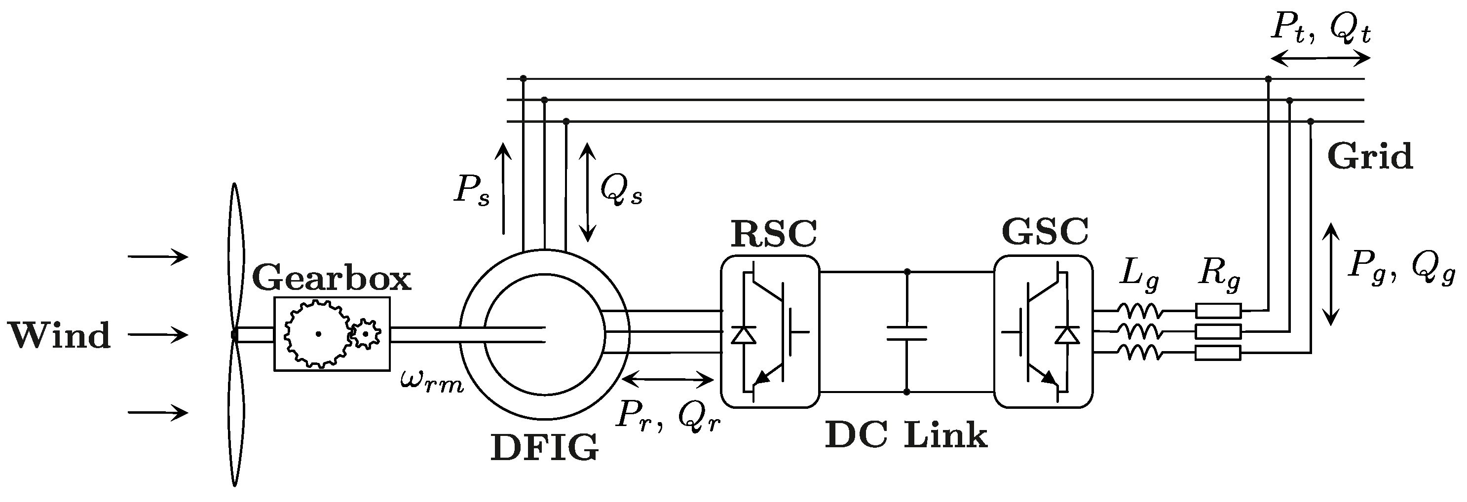
Figure 1 shows the general structure of a DFIG-based wind turbine. Like any other wind turbine topology able to operate at variable speed, in addition to the electric generator, it is equipped with a power converter stage which, when adequately commanded, enables full control of the active and reactive powers interchanged with the electricity grid. Thereby, the stator of the generator is directly connected to the grid, whereas its rotor is linked to the power converter stage. Essentially, the latter comprises two identical three-phase, two-level VSCs—named the rotor-side converter (RSC) and the GSC—linked to each other by means of a DC bus. Likewise, the GSC is connected to the electricity grid through an L-type filter.

Although each power converter possesses its own control algorithm, certain co-ordination between them is required to satisfy the specific control targets, related to the overall wind turbine performance, that arise during electricity network disturbances.

Even if the present study is solely focused on the GSC control algorithm, the control goals of both converters are detailed next, aiming at providing a clear insight into the task of controller parameter tuning that is to be faced.

2.1.1. RSC and GSC Control Targets

The RSC control system is in charge of governing the active and reactive powers interchanged between the stator of the generator and the grid ($P_s$ and $Q_s$, respectively). According to the maximum power point tracking (MPPT) curve [20], the higher the speed of rotation of the wind turbine, the higher the average value of the stator active power set-point, $P_{sav}^{*}$, should be.

During grid disturbances (e.g., imbalances, harmonics, or both) though, in order to prevent harmful fluctuations in the electromagnetic torque of the generator, it is necessary to add an oscillating active power component to the aforementioned set-point average value. Accordingly, the reference value of the stator active power can be expressed as the sum of two terms; that is, $P_s^{*}=P_{sav}^{*}+P_{sosc}^{*}$.

In contrast, the stator reactive power set-point, $Q_s^{*}$, does not fluctuate and, unless the system operator asks for a different value, it is kept near to zero most of the time. This guarantees a power factor close to unity.

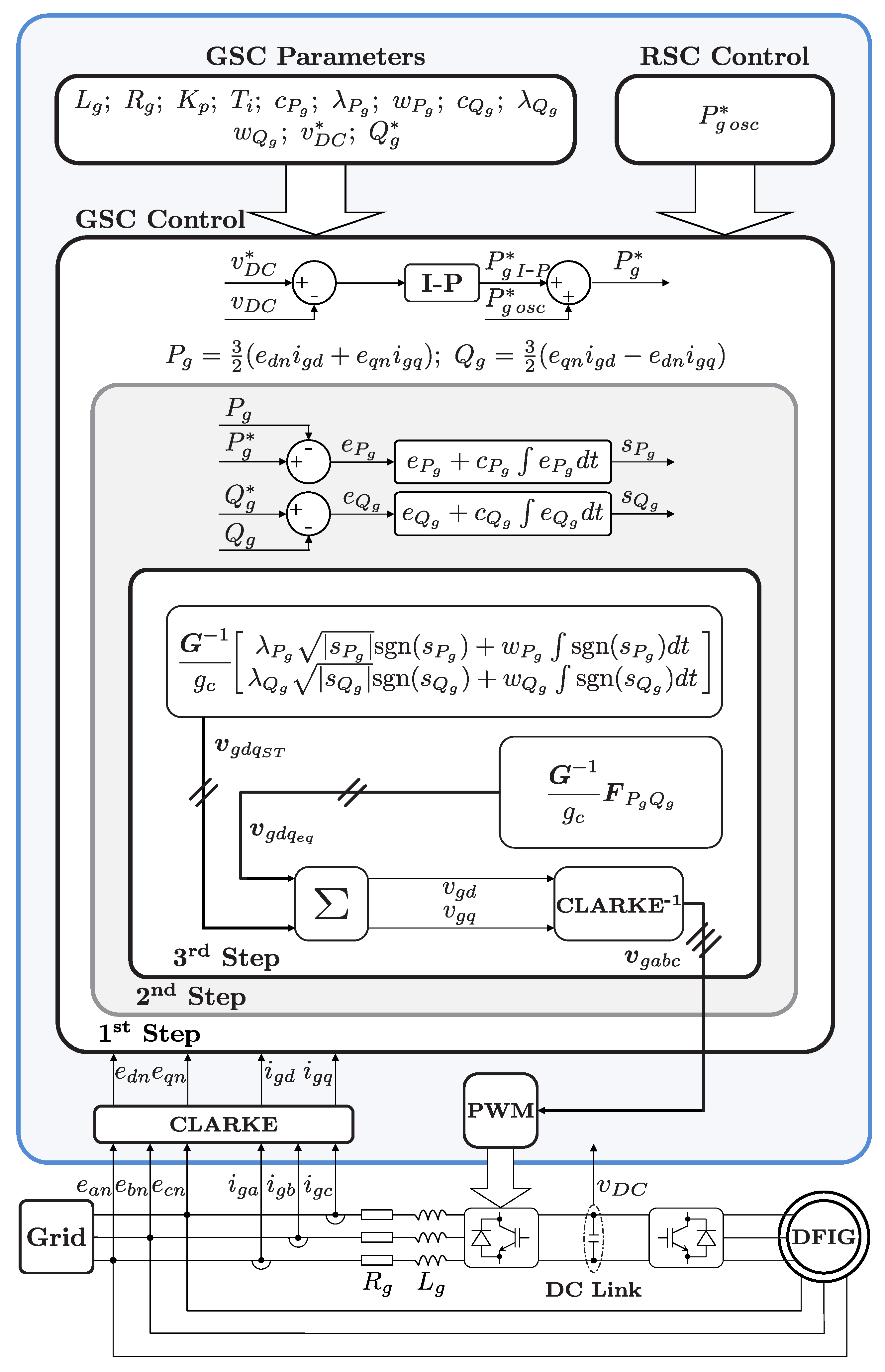
With regard to the GSC control system, it is designed to command the instantaneous active and reactive powers flowing between the GSC and the grid ($P_g$ and $Q_g$, respectively). In particular, the functional diagram displayed in Figure 2 corresponds to the GSC control algorithm adopted in this work, where “CLARKE” and “CLARKE ${}^{-1}$” stand for the Clarke’s and inverse Clarke’s transforms, respectively [21]. This algorithm must be implemented from the outer to the inner layer of the diagram; labelled, respectively, as “1st Step” and “3rd Step” at their bottom left-hand corners. In coherence with the latter, it is assumed that any variable present in a given layer of the diagram is also available to the layers inside.

As in many other works [11], the active power set-point, $P_g^{*}$, is established by an integral-proportional (I-P) controller aimed at keeping the DC-link voltage steady at its rated value. Again, the reactive power set-point, $Q_g^{*}$, is usually fixed to zero under non-faulty conditions.

Pushed by increasingly demanding grid codes, during grid voltages subject to imbalances or harmonic pollution, the GSC control system accomplishes additional control targets, the following two being the most common, as well as incompatible with each other [11,22,23]:

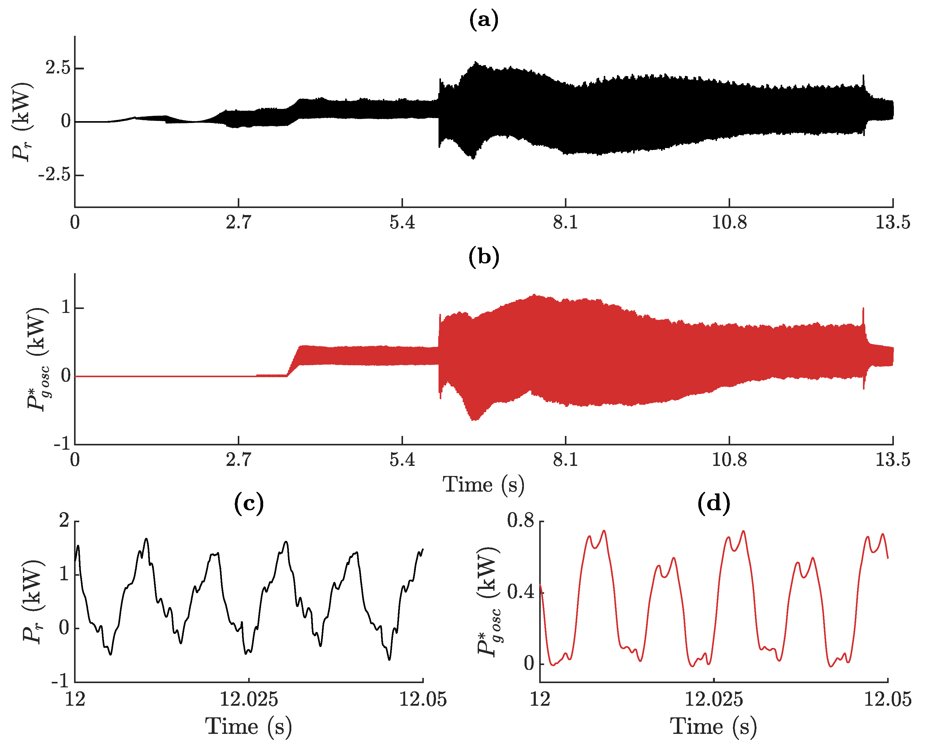
• To add on an oscillating active power term, $P_{gosc}$, that compensates for the above-mentioned oscillatory component of the stator active power, $P_{sosc}$, at the point where the DFIG is connected to the grid. As a result, a non-fluctuating total active power, $P_t=P_s+P_g$, is achieved by the whole wind turbine.
• To compensate the stator current imbalance and/or harmonic distortion, if any, thus balancing the overall current injected by the wind turbine into the grid and/or decreasing its THD as far as possible, respectively.

The first strategy is precisely the one adopted throughout this paper. As a result, not only the total active and reactive powers, $P_t$ and $Q_t$, remain free of fluctuations, but also DC-link voltage oscillations are avoided (which is not possible with the second strategy). In return, in comparison with the approach numbered above as 2, the THD of the overall current injected into the grid turns out to be higher.

Thereby, for the selected strategy, the reference value of the grid-side active power is computed as follows [11]:

$$\begin{array}{cc}\hfill P_g^{*}& =P_{gI-P}^{*}+P_{gosc}^{*},\hfill \end{array}$$

(1)

where $P_{gosc}^{*}$ depends on variables related to the electric generator, and may be estimated as

$$\begin{array}{cc}\hfill P_{gosc}^{*}& =T_e{\omega }_{rm}-P_s,\hfill \end{array}$$

(2)

with $T_e$ and ${\omega }_{rm}$ being the generator electromagnetic torque and rotational speed, respectively.

The output of each power converter’s control system is the three-phase voltage, to be applied by said converter at its AC side. Thus, fixing the appropriate three-phase AC voltage, the aforementioned active and reactive powers can be governed. However, as is usual in three-phase AC power systems, both the RSC and GSC control algorithms are designed, as well as run, in the so-called vector space.

Thus, it is important to clarify that, in the case at hand, the control signals generated by the 2-SMC algorithm under study correspond to the stationary-frame d-q components of the GSC output voltage.

2.1.2. GSC and Grid Filter Modelling

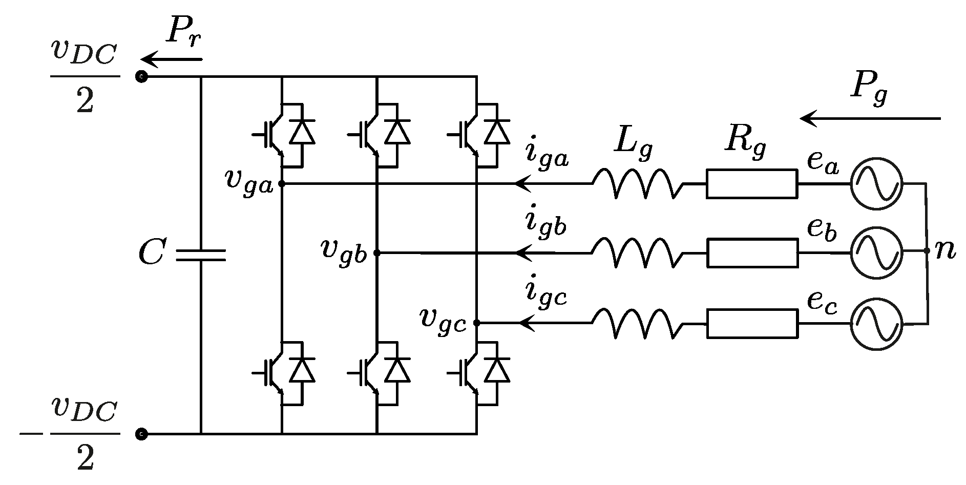
According to Figure 3, adopting the rectifier convention and expressing all variables in the stationary reference frame, the grid-side active and reactive powers can be derived as follows:

$$\begin{array}{cc}\hfill P_g& =\frac{3}{2}\left(e_{dn}{i}_{gd}+e_{qn}{i}_{gq}\right)\hfill \end{array}$$

(3)

$$\begin{array}{cc}\hfill Q_g& =\frac{3}{2}\left(e_{qn}{i}_{gd}-e_{dn}{i}_{gq}\right),\hfill \end{array}$$

(4)

with $e_{dn}$, $e_{qn}$, and $i_{gd}$, $i_{gq}$ being, respectively, the direct- and quadrature-axis components of the grid voltage and current. The dynamics of the latter have been provided, in [11], as

$$\begin{array}{cc}\hfill {\dot{i}}_{gd}& =\frac{1}{L_g}\left(e_{dn}-v_{gd}-R_g{i}_{gd}\right)\hfill \end{array}$$

(5)

$$\begin{array}{cc}\hfill {\dot{i}}_{gq}& =\frac{1}{L_g}\left(e_{qn}-v_{gq}-R_g{i}_{gq}\right),\hfill \end{array}$$

(6)

where $v_{gd}$ and $v_{gq}$ denote the outputs of the GSC control algorithm, while $R_g$ and $L_g$ represent the equivalent resistance and inductance of the grid filter, respectively. Given that such filter is assumed to be of type L, $R_g$ is typically close to zero.

2.2. 2-SMC Scheme Adopted for the GSC

2.2.1. Switching Functions Selected

Considering that $P_g$ and $Q_g$ are the variables to be controlled, the following two switching functions are defined:

$$\begin{array}{cc}\hfill s_{P_g}& =\stackrel{e_{P_g}}{\overbrace{P_g^{*}-P_g}}+c_{P_g}{\int }_0^t{e}_{P_g}(\tau )d\tau \hfill \end{array}$$

(7)

$$\begin{array}{cc}\hfill s_{Q_g}& =\underset{e_{Q_g}}{\underbrace{Q_g^{*}-Q_g}}+c_{Q_g}{\int }_0^t{e}_{Q_g}(\tau )d\tau ,\hfill \end{array}$$

(8)

where the integral terms are aimed at steering possible steady-state errors to zero [24]. Regarding the weighting constants $c_{P_g}$ and $c_{Q_g}$, which need to be tuned, two alternatives will be explored in this paper; namely:

• To assume they both can take any strictly positive value. Specifically, MOO is applied in this work in order to select $c_{P_g}$ and $c_{Q_g}$ from within a wide range of possible values.
• To force them to zero, hence simplifying both switching functions and, in turn, the global control scheme for the GSC.

2.2.2. Control Laws

Taking the time derivatives of Equations (7) and (8), and making use of Equations (3)–(6), the following dynamics arise for the switching functions $s_{P_g}$ and $s_{Q_g}$:

$$\left[\begin{array}{c}{\dot{s}}_{P_g}\\ {\dot{s}}_{Q_g}\end{array}\right]=\underset{{\mathit{F}}_{P_g{Q}_g}}{\underbrace{\left[\begin{array}{c}{F}_{P_g}\\ F_{Q_g}\end{array}\right]}}-\frac{3}{2L_g}\underset{\mathit{G}}{\underbrace{\left[\begin{array}{cc}-e_{dn}& -e_{qn}\\ -e_{qn}& e_{dn}\end{array}\right]}}\left[\begin{array}{c}{v}_{gd}\\ v_{gq}\end{array}\right],$$

(9)

where

$$\begin{array}{cc}\hfill F_{P_g}& ={\dot{P}}_g^{*}-\frac{3}{2}\left({\dot{e}}_{dn}{i}_{gd}+{\dot{e}}_{qn}{i}_{gq}\right)-\frac{3}{2L_g}\left(e_{dn}^2+e_{qn}^2\right)+\frac{R_g}{L_g}{P}_g+c_{P_g}{e}_{P_g}\hfill \end{array}$$

(10)

$$\begin{array}{cc}\hfill F_{Q_g}& ={\dot{Q}}_g^{*}-\frac{3}{2}\left({\dot{e}}_{qn}{i}_{gd}-{\dot{e}}_{dn}{i}_{gq}\right)+\frac{R_g}{L_g}{Q}_g+c_{Q_g}{e}_{Q_g}.\hfill \end{array}$$

(11)

As proposed in [11], the control signals $v_{gd}$ and $v_{gq}$ are computed as a summation of two terms; namely:

• The ${\mathit{v}}_{gd{q}_{ST}}$ “super-twisting” (ST) control term, intended to attain high-performance closed-loop dynamics, ability for disturbance rejection, and robustness in the face of uncertainties, both structured and unstructured.
• The ${\mathit{v}}_{gd{q}_{eq}}$ equivalent control term, incorporated with the main purpose of reducing the control effort to be made by the ST algorithm.

The preceding approach may be mathematically expressed as

$$\underset{{\mathit{v}}_{gdq}}{\underbrace{\left[\begin{array}{c}{\mathit{v}}_{gd}\\ v_{gq}\end{array}\right]}}=\underset{{\mathit{v}}_{gd{q}_{eq}}}{\underbrace{\left[\begin{array}{c}{v}_{g{d}_{eq}}\\ v_{g{q}_{eq}}\end{array}\right]}}+\underset{{\mathit{v}}_{gd{q}_{ST}}}{\underbrace{\left[\begin{array}{c}{v}_{g{d}_{ST}}\\ v_{g{q}_{ST}}\end{array}\right]}}.$$

(12)

After forcing ${\dot{s}}_{P_g}={\dot{s}}_{Q_g}=0$ in Equation (9), the equivalent control term is derived by simply solving for $v_{gd}$ and $v_{gq}$ in said expression, which gives rise to

$${\mathit{v}}_{gd{q}_{eq}}=\frac{2}{3}{L}_g{\mathit{G}}^{-1}{\mathit{F}}_{P_g{Q}_g}=\frac{2L_g}{3\underset{{\left|{\mathit{e}}_n\right|}^2}{\underbrace{\left(e_{dn}^2+e_{qn}^2\right)}}}\left[\begin{array}{cc}-e_{dn}& -e_{qn}\\ -e_{qn}& e_{dn}\end{array}\right]{\mathit{F}}_{P_g{Q}_g},$$

(13)

where the matrix $\mathit{G}$ is invertible, except for the case in which $\left|{\mathit{e}}_n\right|=0$, corresponding to a null grid voltage. Assuming that the sliding regime is reached (i.e., $s_{P_g}=s_{Q_g}=0$), ${\mathit{v}}_{gd{q}_{eq}}$ would allow for preserving it in the absence of disturbances, as well as under both parametric and modelling uncertainties.

However, depending on the specific shapes of both $P_g^{*}$ and $Q_g^{*}$, their respective ${\dot{P}}_g^{*}$ and ${\dot{Q}}_g^{*}$ time derivatives, present in ${\mathit{F}}_{P_g{Q}_g}$ by virtue of Equations (10) and (11), are likely to bring noise, and even derivative kicks, into the ${\mathit{v}}_{gd{q}_{eq}}$ equivalent control term. Therefore, in order to elude such a jeopardy, ${\dot{P}}_g^{*}={\dot{Q}}_g^{*}=0$ is considered in Equation (13) [22].

In any case, the inaccuracies made due to that design simplification, as well as the high parameter dependency evidenced by the equivalent control in Equation (13), do not compromise the robustness of the global control algorithm in Equation (12), as said robustness relies on the ST control term that follows:

$${\mathit{v}}_{gd{q}_{ST}}=\frac{2}{3}{L}_g{\mathit{G}}^{-1}{\mathit{v}}_{P_g{Q}_{gST}}=\frac{2L_g}{3{\left|{\mathit{e}}_n\right|}^2}\left[\begin{array}{cc}-e_{dn}& -e_{qn}\\ -e_{qn}& e_{dn}\end{array}\right]{\mathit{v}}_{P_g{Q}_{gST}},$$

(14)

with

$${\mathit{v}}_{P_g{Q}_{gST}}=\left[\begin{array}{c}{v}_{P_{gST}}\\ v_{Q_{gST}}\end{array}\right]=\left[\begin{array}{c}{\lambda }_{P_g}\sqrt{\left|s_{P_g}\right|}\mathrm{sgn}\left(s_{P_g}\right)+w_{P_g}{\int }_0^t\mathrm{sgn}\left(s_{P_g}(\tau )\right)d\tau \\ {\lambda }_{Q_g}\sqrt{\left|s_{Q_g}\right|}\mathrm{sgn}\left(s_{Q_g}\right)+w_{Q_g}{\int }_0^t\mathrm{sgn}\left(s_{Q_g}(\tau )\right)d\tau \end{array}\right].$$

(15)

The terms of the form ${\lambda }_x\sqrt{\left|s_x\right|}\mathrm{sgn}\left(s_x\right)$, where $x=P_g$ or $Q_g$, are responsible for ensuring the achievement of the sliding regime in finite time.

It should be noted that there are six parameters to be tuned; namely: $c_{P_g}$, ${\lambda }_{P_g}$, $w_{P_g}$, $c_{Q_g}$, ${\lambda }_{Q_g}$, and $w_{Q_g}$. Nonetheless, as already stated at the end of Section 2.2.1, the option of forcing $c_{P_g}=c_{Q_g}=0$ will also be explored, which leads to a simplified version of the GSC control algorithm with just four parameters: ${\lambda }_{P_g}$, $w_{P_g}$, ${\lambda }_{Q_g}$, and $w_{Q_g}$.

2.3. Multi-Objective Optimisation

A MOOP with m objectives to minimise can be stated as follows [25]:

$$\underset{\mathit{x}}{min}\mathit{f}(\mathit{x})$$

(16)

subject to

$$\begin{array}{ccc}\hfill \mathit{K}(\mathit{x})\le 0& ,& \mathit{L}(\mathit{x})=0\hfill \end{array}$$

(17)

$$\begin{array}{ccc}\hfill \underline{x_i}\le x_i\le \overline{x_i}& ,& i=[1,2\dots n],\hfill \end{array}$$

(18)

where $\mathit{x}=[x_1,x_2\dots x_n]\in D$ is the decision vector, with $dim(\mathit{x})=n$; $\mathit{f}(\mathit{x})=[f_1(\mathit{x}),f_2(\mathit{x})\cdots f_m(\mathit{x})]$ is the objective vector; $\mathit{K}(\mathit{x})$ and $\mathit{L}(\mathit{x})$ are the inequality and equality constraint vectors, respectively; and $\underline{x_i}$ and $\overline{x_i}$ are the lower and upper bounds in the D decision space, respectively.

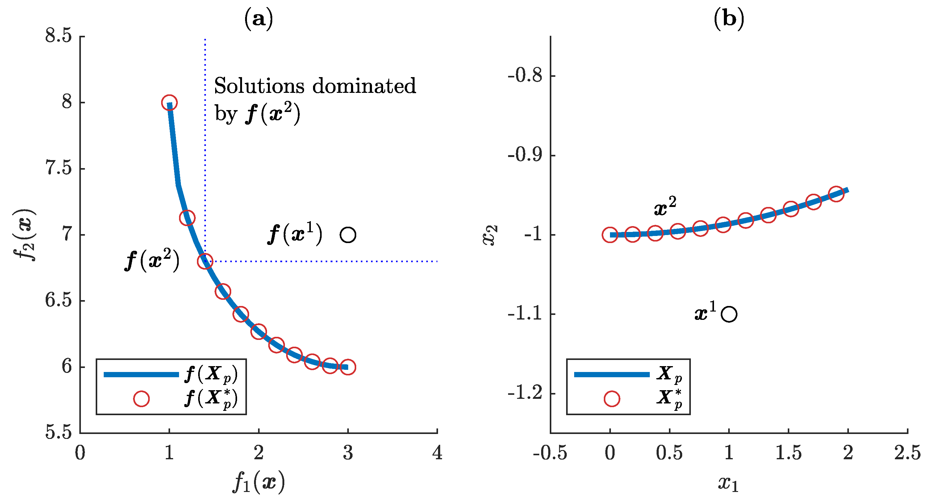
As the objectives of a MOOP are usually in opposition, there is typically no single solution that minimises all the objectives. Instead, there will exist a set of Pareto optimal solutions (i.e., non-dominated solutions).

Definition 1.

(Pareto optimality [25]): An objective vector $\mathit{f}({\mathit{x}}^2)$ is Pareto optimal if there is no other objective vector $\mathit{f}({\mathit{x}}^1)$ such that $f_i({\mathit{x}}^1)\le f_i({\mathit{x}}^2)$ for all $i\in [1,2\dots m]$ and $f_j({\mathit{x}}^1)<f_j({\mathit{x}}^2)$, for at least one j, $j\in [1,2\dots m]$.

Definition 2.

(Dominance [26]): An objective vector $\mathit{f}({\mathit{x}}^1)$ is dominated by another objective vector $\mathit{f}({\mathit{x}}^2)$ iff $f_i({\mathit{x}}^2)\le f_i({\mathit{x}}^1)$ for all $i\in [1,2\cdots m]$ and $f_j({\mathit{x}}^2)<f_j({\mathit{x}}^1)$, for at least one j, $j\in [1,2\dots m]$. This is denoted as $\mathit{f}({\mathit{x}}^2)⪯\mathit{f}({\mathit{x}}^1)$.

Therefore, the set of solutions (the Pareto set) is defined as follows:

Definition 3.

(Pareto set, ${\mathit{X}}_p$): The Pareto set is the set of all solutions in D that are not dominated by any other solution in D:

$${\mathit{X}}_p:=\{\mathit{x}\in D|\nexists {\mathit{x}}^{{}^{\prime }}\in D:\mathit{f}({\mathit{x}}^{{}^{\prime }})⪯\mathit{f}(\mathit{x})\}.$$

Each solution in the Pareto set defines an objective vector in the Pareto front.

Definition 4.

(Pareto front, $\mathit{f}({\mathit{X}}_p)$): Given a set of Pareto optimal solutions ${\mathit{X}}_p$, the Pareto front is defined as

$$\mathit{f}({\mathit{X}}_p):=\left\{\mathit{f}(\mathit{x})\right|\mathit{x}\in {\mathit{X}}_p\}.$$

Usually, ${\mathit{X}}_p$ contains an infinite number of solutions and, for this reason, it is not possible to completely obtain it. The way to proceed is to obtain a discrete set ${\mathit{X}}_p^{*}\subset {\mathit{X}}_p$, in such a way that ${\mathit{X}}_p^{*}$ characterises ${\mathit{X}}_p$. Note that the set ${\mathit{X}}_p^{*}$ is not unique. In this work, the ev-MOGA algorithm (Available at https://es.mathworks.com/matlabcentral/fileexchange/31080-ev-moga-multiobjective-evolutionary-algorithm) [13] will be used to obtain the Pareto front approximations. Figure 4 shows an example of characterisation of a bi-objective Pareto front and its corresponding Pareto set.

2.4. Comparison of Design Concepts Under MOO Approach

It is very common that several design alternatives (i.e., design concepts), C, are proposed, in order to solve a specific problem. Each design concept might, for example, represent a different control structure. Comparing the different concepts in a multi-objective scenario allows for differentiating the strengths and weaknesses of each of them, in relation to the chosen objectives [25,27]. To do so, a MOOP is set for each design concept, $Cj$, such that all MOOPs share the same objectives, $\mathit{f}$, but each of them has its own decision vector, ${\mathit{x}}^{Cj}$, related to the parameterisation of its corresponding design concept. Therefore, if s design concepts need to be compared, the MOOPs can be stated as

$$\underset{{\mathit{x}}^{Cj}}{min}\mathit{f}({\mathit{x}}^{Cj})$$

(19)

subject to

$$\begin{array}{ccc}\hfill {\mathit{K}}^{Cj}({\mathit{x}}^{Cj})\le 0& ,& {\mathit{L}}^{Cj}({\mathit{x}}^{Cj})=0\hfill \end{array}$$

(20)

$$\begin{array}{ccc}\hfill \underline{x_i^{Cj}}\le x_i^{Cj}\le \overline{x_i^{Cj}}& ,& i=[1,2\dots n^{Cj}],\hfill \end{array}$$

(21)

with $j\in [1,2\dots s]$. For each design concept, ${\mathit{x}}^{Cj}=[x_1^{Cj},x_2^{Cj}\dots x_{n^{Cj}}^{Cj}]$ is the decision vector; ${\mathit{K}}^{Cj}({\mathit{x}}^{Cj})$ and ${\mathit{L}}^{Cj}({\mathit{x}}^{Cj})$ are the inequality and equality constraint vectors, respectively; and $\underline{x_i^{Cj}}$ and $\overline{x_i^{Cj}}$ are the lower and upper bounds delimiting the searching space, respectively. In contrast, the objective vector $\mathit{f}({\mathit{x}}^{Cj})=[f_1({\mathit{x}}^{Cj}),f_2({\mathit{x}}^{Cj})\cdots f_m({\mathit{x}}^{Cj})]$ is common to the s MOOPs.

After optimising each multi-objective problem, a discrete Pareto set, ${\mathit{X}}_p^{*Cj}$, and its corresponding Pareto front, $\mathit{f}({\mathit{X}}_p^{*Cj})$, are obtained for each design concept. Thanks to the fact that all of the MOOPs share the same objectives, a comparison in the m-objective space can be made. This idea is illustrated in Figure 5, where the Pareto fronts of three design concepts are depicted in a bi-objective optimisation problem. By analysing the figure, it is possible to notice the following:

• Design concept 3 is dominated by design concepts 1 and 2. Therefore, the latter two will be preferred.
• Depending on designer preferences, design concept 1 or 2 may be preferred.
• Zone C (values of $f_2(\mathit{x})<6.06$) is only reachable by design concept 2. Consequently, if the designer demands such a trade-off, design concept 2 would be the right one.
• In Zone B ($f_1(\mathit{x})\in [1.7,2.5]$), design concept 2 dominates design concept 1. As a result, design concept 2 will be preferred over design concept 1.
• The opposite to what occurs in Zone B is observable in Zone A ($f_1(\mathit{x})<1.7$). Design concept 2 is dominated by design concept 1 and, thus, the latter will be preferred.

2.5. LDs for Design Concept Comparison

In order to efficiently compare design concepts in an m-dimensional objective space, an adequate visualisation method is required. Among the several methods provided in the literature [28], the interactive tool referred to as LDs [15,16,29] is employed in this work.

The LD tool (Available at https://es.mathworks.com/matlabcentral/fileexchange/62224-interactive-tool-for-decision-making-in-multiobjective-optimization-with-level-diagrams) transforms the m-dimensional objective space and the n-dimensional decision space into $m+n$ two-dimensional separate (but synchronised) graphs. For that purpose, first, each point of the Pareto fronts $\mathit{f}({\mathit{x}}^{Cj})$ is normalised with respect to the ideal ${\mathit{f}}^{ideal}$ and nadir ${\mathit{f}}^{nadir}$ points (see Figure 5), as given below:

$${\widehat{f}}_i({\mathit{x}}^{Cj})=\frac{f_i({\mathit{x}}^{Cj})-f_i^{ideal}}{f_i^{nadir}-f_i^{ideal}},i\in [1,2\cdots m].$$

(22)

Second, the p-norm $\parallel \widehat{\mathit{f}}({\mathit{x}}^{Cj}){\parallel }_p$ is applied to each normalised point. Typical norms are: (1) Taxicab norm—also called Manhattan norm—, $p=1$; (2) Euclidean norm, $p=2$; and (3) infinity norm—also known as maximum norm—, $p=\infty$.

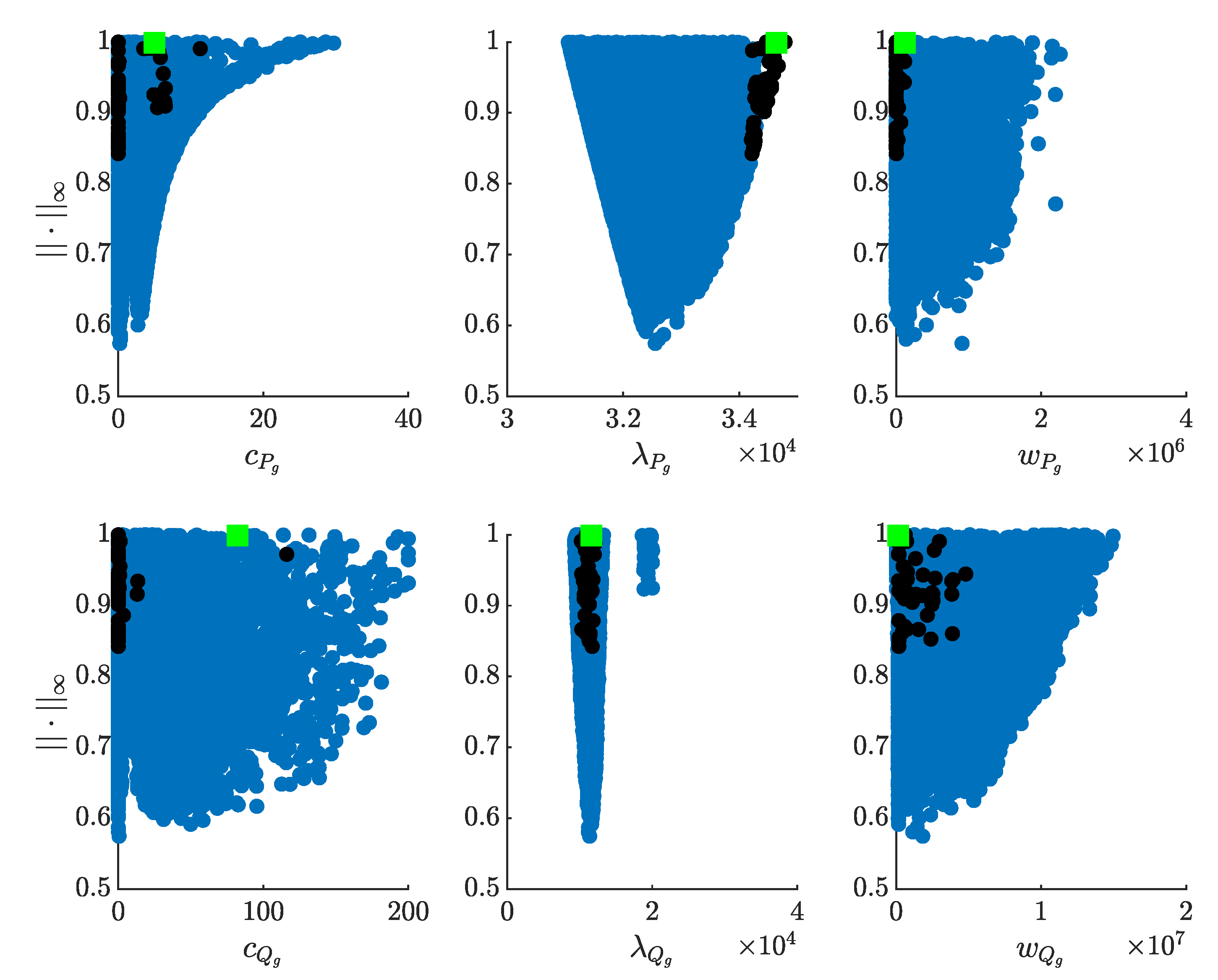
After that, the LD tool provides a two-dimensional graph for each objective and decision variable. On the abscissa axis of each graph, the values for each objective or decision variable are represented, while the ordinate axes of all graphs display the p-norm previously calculated for each solution. The latter allows graphics to stay synchronised, by means of their ordinate axes (meaning that each given solution of a design concept presents identical ordinate value in every graph) and, therefore, helps to compare solutions according to the selected norm.

Adopting the Euclidean norm, Figure 6 shows the LD corresponding to the same three design concepts presented in Figure 5. Given that, similarly to Figure 5, the search space is not contemplated, only two graphs associated to the objective space are provided, which corresponds to the bi-objective problem considered. The A, B, and C zones have been marked, in order to demonstrate their correspondence with the same zones displayed in Figure 5. It can be noticed that the solutions of design concept 2 are the closest to ${\mathit{f}}^{ideal}$, as they present lower values of $\parallel \widehat{\mathit{f}}{\parallel }_2$.

Two solutions, ${\mathit{x}}^{C1,A}$ from design concept 1 and ${\mathit{x}}^{C2,B}$ from design concept 2, have been highlighted. Although they both present low values of $f_1$ and high values of $f_2$, it is clearly observable that ${\mathit{x}}^{C1,A}$ dominates ${\mathit{x}}^{C2,B}$. It should be noted that, when more than three objectives are considered, it becomes difficult to appreciate such relations using classical visualisation tools.

3. Framework for MOO Tuning of the GSC Control Scheme

3.1. Simulation Test Designed

The proposed MOO-based tuning methodology, requiring a considerable amount of simulations to run, was applied on the 7 kW DFIG prototype employed in [11] for experimentation.

To that end, each new set of values to be tested for the GSC controller parameters (i.e., $c_{P_g}$, ${\lambda }_{P_g}$, $w_{P_g}$, $c_{Q_g}$, ${\lambda }_{Q_g}$, and $w_{Q_g}$) was evaluated on a simulation model reproducing the grid-connected GSC and the DC bus of the 7 kW DFIG prototype, as well as the DC bus $v_{DC}$ voltage I-P regulator. Its parameters are provided in

Table 1. Parameters of the 7 kW DFIG grid filter, DC bus, and $v_{DC}$ I-P regulator.

Parameter	Value
$R_g$	0 m$\Omega$
$L_g$	2 mH
C	9.4 mF
$v_{DC}$	125 V
$K_p$	45.4333 W/V
$T_i$	103.4483 ms

, where the equivalent $R_g$ resistance of the L-type grid filter was assumed to be negligible.

Considering the high amount of simulation tests to run, it is essential to keep in mind that significantly higher simulation times are required if commutation of the GSC transistors is to be reproduced by the model. Consequently, the PWM–GSC set displayed in Figure 2 is treated as if its operation was ideal, by assuming that the three-phase ${\mathit{v}}_{gabc}$ voltage applied by the GSC to the grid filter coincides exactly with that computed by its control scheme. In this way, the simulation times were drastically reduced while preserving impartiality of the comparisons, as the described simplification affected equally any parameter set to be evaluated.

It is intended that a unique set of controller parameters remains valid for a good number of representative DFIG operating regimes. For that purpose, the simulation test based on which the tuning process is tackled pushes the DFIG to transit, one after another, through the nine different stages collected and described in

Table 2. Stages of the designed test.

Time Range	Stage	Description
$t_0$–$t_1$	1	With the DFIG stator disconnected from the grid, transient of charge of the DC bus until its rated voltage is reached.
$t_1$–$t_2$	2	With its stator disconnected from the grid, initial positioning of the DFIG rotor.
$t_2$–$t_3$	3	With the DFIG stator disconnected from the grid, synchronisation of the voltage induced in the terminals of said open stator with the grid voltage.
$t_3$–$t_4$	4	Smooth connection (with no power or zero power exchange) of the DFIG stator to the grid at time $t_3$, and maintenance of said zero power for the entire $t_3$–$t_4$ interval.
$t_4$–$t_5$	5	Starting from zero power at time $t_4$, the power generated by the DFIG ramps up to its optimum value, which is reached at time $t_5$.
$t_5$–$t_6$	6	Generation of the optimum power corresponding to the DFIG rotor speed at which the test is carried out.
$t_6$–$t_7$	7	A two-phase E-type imbalance affects the grid voltage between time instants $t_6$ and $t_8$. This $t_6$–$t_7$ time interval corresponds to the transient following the start of said imbalance.
$t_7$–$t_8$	8	Steady state resulting from the two-phase E-type imbalance.
$t_8$–$t_9$	9	Transient following the conclusion of the two-phase E-type imbalance.

. The specific values assigned to the different time instants displayed in Table 2 are provided in

Table 3. Values for the time instants delimiting the stages of the designed test.

Time Instant	${\mathit{t}}_0$	${\mathit{t}}_1$	${\mathit{t}}_2$	${\mathit{t}}_3$	${\mathit{t}}_4$	${\mathit{t}}_5$	${\mathit{t}}_6$	${\mathit{t}}_7$	${\mathit{t}}_8$	${\mathit{t}}_9$
Value (s)	0	0.5	2	3	3.5	3.7033	6	11.3	13	13.5

.

In order to run simulations under realistic conditions of harmonic pollution, the three-phase $e_{an}$, $e_{bn}$, and $e_{cn}$ grid voltage profile adopted for simulation was registered in the laboratory housing the 7 kW DFIG prototype. A detail suggesting the level of harmonic distortion present in said grid voltage profile is provided in Figure 7a. Furthermore, in accordance with Table 2 and Table 3, such a grid voltage profile also presents a two-phase E-type imbalance of approximately 15% between time instants $t_6=6$ and $t_8=13$ s, as evidenced by Figure 7b,c.

Concerning the effect of the RSC, it was incorporated into the so-far described simulation model by means of a disturbance representing the rotor active power, $P_r$, as shown in Figure 3. In particular, Figure 8a displays the specific $P_r$ profile under which every set of GSC controller parameters considered was tested. Consequently, fairness of comparisons is preserved, as all possible sets of GSC controller parameters were evaluated under identical conditions.

As far as grid power reference values are concerned, $Q_g^{*}$ was set to zero, while $P_g^{*}$ was derived by adding the feedforward $P_{gosc}^{*}$ term displayed in Figure 8b to the control signal generated by the DC bus voltage I-P regulator, as dictated by Equations (1) and (2), and as represented in Figure 2. An 100 Hz oscillation in both $P_r$ and $P_{gosc}^{*}$ indicative of the presence of a negative sequence and, in turn, of an imbalance in the grid voltage, is made visible in the detail of Figure 8c,d.

In order to derive the $P_r$ and $P_{gosc}^{*}$ profiles in Figure 8a,b, the test described in Table 2 was first run on a complete simulation model, reproducing not only the global 7 kW DFIG prototype considered in [11], but also its RSC and GSC control schemes, tuned as explicitly stated in Table 2 of said paper. It should be pointed out that the angular speed of the DFIG was kept constant, at 1320 rpm, during the entire test. This way, it was sought that the disturbance due to the wind speed variability affected the nine operating regimes equally, as the value of ${\omega }_{rm}$ is a direct consequence of the wind speed.

3.2. Indices Selected

Bearing in mind the two control targets specified for the GSC in Section 2.1.1, as well as the nine different DFIG operating regimes tackled, the following four considerations were made in order to define the performance indices on which the MOOP to be solved was based:

• As evidenced by Equations (1) and (2), if the grid voltage is harmonically distorted or/and unbalanced, a strongly fluctuating $P_g^{*}$ reference must be closely tracked by the active power $P_g$. Accordingly, the performance index referred to as IAE seems suited for determining the quality of tracking achieved.
• Reactive power $Q_g$ has to be regulated around 0. Consequently, deviations of $Q_g$ from 0 and, as a result, the level of chatter in $Q_g$ may be somehow quantified by means of a SD index.
• The two indices suggested above are to be computed for each of the nine stages of the simulation test described in Table 2, thus giving rise to $2\times 9=18$ indices in total. Given that the nine DFIG operating regimes considered are significantly different from each other, computing a single IAE and a single SD for the entire test leads to a loss of valuable information and skews the results [30].
• As the IAE index is cumulative, it is highly dependent on the time interval over which it is calculated. For that reason, the IAE index computed for each of the nine test stages is divided by its corresponding time interval, so that the resulting nine “IAE per unit of time” indices are equitably comparable with each other.

As a consequence, the 18 performance indices considered were as follows:

$$\begin{array}{cc}\hfill f_{{P_g}_i}& =\frac{IA{E}_{{P_g}_i}}{t_i-t_{i-1}}=\frac{{\int }_{t_{i-1}}^{t_i}\left|{P_g}^{*}-P_g\right|dt}{t_i-t_{i-1}};i\in [1,2,3\dots 9]\hfill \end{array}$$

(23)

$$\begin{array}{cc}\hfill f_{{Q_g}_i}& =S{D}_{{Q_g}_i};i\in [1,2,3\dots 9],\hfill \end{array}$$

(24)

where the i subscript accompanying a given performance index indicates the index to correspond to the ith stage of the test.

3.3. Statement of the MOOP

In brief, the objective consists of minimising the 18 indices established in Equations (23) and (24) by properly tuning the parameters of the 2-SMC scheme, commanding both $P_g$ and $Q_g$. As indicated at the end of Section 2.2.2, two alternative 2-SMC structures were actually considered; that is,

• Design concept 1: All the six controller parameters (explicitly listed at the end of Section 2.2.2) are assumed to be strictly positive (non-zero). Hence, the vector of controller parameters to be adjusted is given by

  $${\mathit{x}}^{C{1}_{6p}}=\left[c_{P_g}{\lambda }_{P_g}{w}_{P_g}{c}_{Q_g}{\lambda }_{Q_g}{w}_{Q_g}\right].$$

  (25)
• Design concept 2: The parameters $c_{P_g}$ and $c_{Q_g}$ are set to zero in Equation (25), thus removing the integral terms from the switching functions in Equations (7) and (8). As a result, only four parameters need to be tuned in this particular case, therefore yielding

  $${\mathit{x}}^{C{2}_{4p}}=\left[{\lambda }_{P_g}{w}_{P_g}{\lambda }_{Q_g}{w}_{Q_g}\right].$$

  (26)

On the other hand, the parameter set

$${\mathit{x}}^{C{1}_{6p},ref}=\left[96.666733.6256\times {10}^{3}23.3611\times {10}^{6}96.666710.6333\times {10}^{3}2.3361\times {10}^6\right],$$

(27)

derived in [11] for the GSC 2-SMC scheme, was adopted as the baseline solution. In particular, only those parameter sets improving each and every one of the 18 indices resulting from application of the baseline solution in Equation (27) will be considered. The values for the indices corresponding to the baseline solution are reflected in

Table 4. Values of the 18 indices produced by ${\mathit{x}}^{C{1}_{6p},ref}$.

i	1	2	3	4	5	6	7	8	9
$f_{{P_g}_i}({\mathit{x}}^{C{1}_{6p},ref})$	83.803	10.144	10.458	10.838	11.312	13.204	25.749	22.653	13.995
$f_{{Q_g}_i}({\mathit{x}}^{C{1}_{6p},ref})$	69.702	3.383	3.576	3.64	5.814	7.368	12.389	11.853	7.852

.

Consequently, the two MOOPs to be solved are formally stated as follows:

• MOOP for design concept 1:

  $${\mathit{X}}_p^{*C{1}_{6p}}=\underset{{\mathit{x}}^{C{1}_{6p}}}{min}\mathit{f}=\underset{{\mathit{x}}^{C{1}_{6p}}}{min}\left[\left[f_{{P_g}_1},f_{{P_g}_2},f_{{P_g}_3}\dots f_{{P_g}_9}\right],\left[f_{{Q_g}_1},f_{{Q_g}_2},f_{{Q_g}_3}\dots f_{{Q_g}_9}\right]\right]$$

  (28)

  subject to constraints

  $$\begin{array}{cc}\hfill f_{{P_g}_i}({\mathit{x}}^{C{1}_{6p}})& \le f_{{P_g}_i}({\mathit{x}}^{C{1}_{6p},ref});i\in [1,2,3\dots 9]\hfill \end{array}$$

  (29)

  $$\begin{array}{cc}\hfill f_{{Q_g}_i}({\mathit{x}}^{C{1}_{6p}})& \le f_{{Q_g}_i}({\mathit{x}}^{C{1}_{6p},ref});i\in [1,2,3\dots 9]\hfill \end{array}$$

  (30)

  $$\underline{{\mathit{x}}^{C{1}_{6p}}}\le {\mathit{x}}^{C{1}_{6p}}\le \overline{{\mathit{x}}^{C{1}_{6p}}},$$

  (31)

  with

  $$\begin{array}{cc}\hfill \underline{{\mathit{x}}^{C{1}_{6p}}}& =\left[0{10}^3{10}^{3}0{10}^3{10}^3\right]\hfill \end{array}$$

  (32)

  $$\begin{array}{cc}\hfill \overline{{\mathit{x}}^{C{1}_{6p}}}& =\left[2005\times {10}^{4}3\times {10}^{7}2005\times {10}^{4}3\times {10}^7\right].\hfill \end{array}$$

  (33)
• MOOP for design concept 2:

  $${\mathit{X}}_p^{*C{2}_{4p}}=\underset{{\mathit{x}}^{C{2}_{4p}}}{min}\mathit{f}=\underset{{\mathit{x}}^{C{2}_{4p}}}{min}\left[\left[f_{{P_g}_1},f_{{P_g}_2},f_{{P_g}_3}\dots f_{{P_g}_9}\right],\left[f_{{Q_g}_1},f_{{Q_g}_2},f_{{Q_g}_3}\dots f_{{Q_g}_9}\right]\right]$$

  (34)

  subject to constraints

  $$\begin{array}{cc}\hfill f_{{P_g}_i}({\mathit{x}}^{C{2}_{4p}})& \le f_{{P_g}_i}({\mathit{x}}^{C{1}_{6p},ref});i\in [1,2,3\dots 9]\hfill \end{array}$$

  (35)

  $$\begin{array}{cc}\hfill f_{{Q_g}_i}({\mathit{x}}^{C{2}_{4p}})& \le f_{{Q_g}_i}({\mathit{x}}^{C{1}_{6p},ref});i\in [1,2,3\dots 9]\hfill \end{array}$$

  (36)

  $$\underline{{\mathit{x}}^{C{2}_{4p}}}\le {\mathit{x}}^{C{2}_{4p}}\le \overline{{\mathit{x}}^{C{2}_{4p}}},$$

  (37)

  with

  $$\begin{array}{cc}\hfill \underline{{\mathit{x}}^{C{2}_{4p}}}& =\left[{10}^3{10}^3{10}^3{10}^3\right]\hfill \end{array}$$

  (38)

  $$\begin{array}{cc}\hfill \overline{{\mathit{x}}^{C{2}_{4p}}}& =\left[5\times {10}^{4}3\times {10}^{7}5\times {10}^{4}3\times {10}^7\right].\hfill \end{array}$$

  (39)

4. Results and Evaluation

In order to perform the two MOOs defined in Equations (28) and (34), ev-MOGA was applied with the following configuration:

• $Nin{d}_P$ = 1000,
• $Nin{d}_G$ = 8,
• $Iterations$ = 5000, and
• $N_{box}$ = 15.

For the definition of the remaining parameters, the default values suggested by [31] were adopted.

4.1. MOO Results and Analysis

As a result of the optimisation process, a Pareto front approximation with 13,649 solutions was obtained for design concept 1 ($\mathit{f}({\mathit{X}}_p^{*C{1}_{6p}})$) and another one containing 6494 solutions for design concept 2 ($\mathit{f}({\mathit{X}}_p^{*C{2}_{4p}})$), hence proving that it is possible to find 2-SMC controllers, for both the six- and four-parameter cases, that outperform the reference 2-SMC controller in each and every objective. Both Pareto fronts are simultaneously displayed in Figure 9 by means of the LD tool with ∞-norm, while their corresponding Pareto sets are provided in Figure 10 and Figure 11 for design concepts 1 (${\mathit{X}}_p^{*C{1}_{6p}}$) and 2 (${\mathit{X}}_p^{*C{2}_{4p}}$), respectively. In addition,

Table 5. Minimum values of the 18 performance indices achievable by the six-parameter controllers of design concept 1.

i	1	2	3	4	5	6	7	8	9
$f_{{P_g}_i}$	41.0553	8.0831	8.0372	8.3810	9.7569	12.2202	21.2045	18.7141	12.9973
$f_{{Q_g}_i}$	4.6689	2.8165	2.9554	3.1834	5.2693	6.3064	10.9742	10.9207	6.7105

and

Table 6. Minimum values of the 18 performance indices achievable by the four-parameter controllers of design concept 2. The five performance indices for which concept 2 does not reach the minimum values attainable by concept 1 are highlighted in bold.

i	1	2	3	4	5	6	7	8	9
$f_{{P_g}_i}$	41.0553	8.0831	8.0372	8.3810	9.7749	12.3491	21.2045	18.7141	13.1103
$f_{{Q_g}_i}$	4.6689	2.8165	2.9554	3.1834	5.2693	6.3064	11.0244	10.9207	7.0129

reflect the respective minimum values reached by $\mathit{f}({\mathit{X}}_p^{*C{1}_{6p}})$ and $\mathit{f}({\mathit{X}}_p^{*C{2}_{4p}})$ for each of the 18 performance indices.

A thoughtful analysis of Figure 9, Figure 10 and Figure 11, as well as of Table 5 and Table 6, leads to the following conclusions:

• Figure 9 shows that the Pareto fronts corresponding to design concepts 1 ($\mathit{f}({\mathit{X}}_p^{*C{1}_{6p}})$) and 2 ($\mathit{f}({\mathit{X}}_p^{*C{2}_{4p}})$) practically overlap, their main differences being enclosed by dashed lines. It can be observed that there exist solutions of design concept 1 presenting a slight improvement, with respect to those of design concept 2, for the objectives $f_{{P_g}_5}$, $f_{{P_g}_6}$, $f_{{P_g}_9}$, $f_{{Q_g}_7}$, and $f_{{Q_g}_9}$, in accordance with that suggested by Table 5 and Table 6. However, it was found that, in return, such solutions lose performance in the objectives $f_{{P_g}_1}$, $f_{{P_g}_8}$, and $f_{{Q_g}_1}$.
• The minimum values of the ∞-norm for design concepts 1 and 2 are, respectively, 0.575 and 0.613 (with a less than 4% difference), which means that the normalised distance to the ideal point, ${\mathit{f}}^{ideal}$, is practically the same.
• Aiming at illustrating the trade-off existing among objectives in more detail for both design concepts, the points of both Pareto fronts yielding lower values in $f_{{P_g}_7}$ were selected (see the black dots in Figure 9). Thanks to the synchronisation between objectives carried out by the LD tool, it becomes evident that the objectives $f_{{P_g}_2}$, $f_{{P_g}_3}$, $f_{{P_g}_4}$, $f_{{P_g}_5}$, $f_{{P_g}_6}$, and $f_{{P_g}_9}$ are in opposition to both $f_{{P_g}_7}$ and $f_{{P_g}_8}$, while no clear opposition is observable between objectives $f_{{Q_g}_i}$ and $f_{{P_g}_i}$.
• As the above-mentioned synchronisation also applies to the decision variables, the controller parameters marked with black dots in Figure 10 and Figure 11 are precisely those leading to the solutions represented by black dots in Figure 9. In particular, analysis of the black dots in Figure 10 reveals that they are grouped around two different values of the parameter $c_{P_g}$ (i.e., $c_{P_g}\simeq 0$ and $c_{P_g}\simeq 5$), whereas the great majority lead to a $c_{Q_g}\simeq 0$. The latter confirms that controllers with $c_{P_g}=c_{Q_g}=0$, corresponding to the four-parameter 2-SMC variant, presented similar features to those of the six-parameter one.

Considering all four aspects above, it can be concluded that, although design concept 1 was slightly better than design concept 2, the greater simplicity of the four-parameter 2-SMC variant, compared to that with six parameters, may encourage the designer to eventually opt for the former.

4.2. Selection of 2-SMC Parameter Sets

In general terms, examination of the LDs displayed in Figure 9 reveals that, excluding the indices corresponding to the first stage of the test ($f_{P_{g_1}}$ and $f_{Q_{g_1}}$), the most unfavourable were those resulting from the seventh and eighth stages. Nevertheless, it should be considered that, while the latter two stages were intrinsic to common operation under non-ideal grid voltage, the former corresponded to a short-duration sporadic operating regime.

Accordingly, it is intended that the parameter sets selected for experimental evaluation correspond to solutions yielding outstanding values for $f_{P_{g_7}}$ and $f_{P_{g_8}}$, as those indices were related to the most demanding, though usual, operating conditions. Under this premise, two parameter sets giving rise to extremely similar $f_{P_{g_7}}$ and $f_{P_{g_8}}$ indices were chosen: One from design concept 1, referred to as ${\mathit{x}}^{C{1}_{6p},A}$ henceforward, and the other from design concept 2, designated as ${\mathit{x}}^{C{2}_{4p},B}$.

In particular, the parameter sets ${\mathit{x}}^{C{1}_{6p},A}$ and ${\mathit{x}}^{C{2}_{4p},B}$ are those leading, respectively, to the performance indices highlighted using green squares and yellow diamonds in the LDs of Figure 9. The exact values for the parameters of said two sets, displayed in Figure 10 and Figure 11 following the same format, are those given as follows:

$$\begin{array}{cc}\hfill {\mathit{x}}^{C{1}_{6p},A}& =\left[534.64\times {10}^{3}121.67\times {10}^{3}82.311.606\times {10}^{3}133.095\times {10}^3\right]\hfill \end{array}$$

(40)

$$\begin{array}{cc}\hfill {\mathit{x}}^{C{2}_{4p},B}& =\left[34.79\times {10}^3{10}^{3}10.91\times {10}^{3}477.355\times {10}^3\right].\hfill \end{array}$$

(41)

The precise values of the objectives that result from adopting parameter sets ${\mathit{x}}^{C{1}_{6p},A}$ and ${\mathit{x}}^{C{2}_{4p},B}$ are those provided in

Table 7. Values of the 18 indices produced by ${\mathit{x}}^{C{1}_{6p},A}$.

i	1	2	3	4	5	6	7	8	9
$f_{{P_g}_i}({\mathit{x}}^{C{1}_{6p},A})$	64.432	10.141	10.005	10.328	11.180	12.950	21.450	19.076	13.616
$f_{{Q_g}_i}({\mathit{x}}^{C{1}_{6p},A})$	10.938	3.337	3.447	3.631	5.623	6.946	11.627	11.397	7.573

and

Table 8. Values of the 18 indices produced by ${\mathit{x}}^{C{2}_{4p},B}$.

i	1	2	3	4	5	6	7	8	9
$f_{{P_g}_i}({\mathit{x}}^{C{2}_{4p},B})$	43.288	10.129	10.098	10.373	11.251	13.050	21.204	18.714	13.633
$f_{{Q_g}_i}({\mathit{x}}^{C{2}_{4p},B})$	21.180	3.218	3.319	3.493	5.581	6.993	11.645	11.327	7.634

, respectively.

4.3. Experimental Evaluation

4.3.1. Description of the Experimental Rig

As already pointed out at the beginning of Section 3.1, the whole tuning study presented in Section 4.1 was based on a simulation model of the 7 kW DFIG prototype adopted in [11] for experimentation. A diagram displaying how the main components of that prototype are connected to each other is depicted in Figure 12a, while the physical aspect of those main components is observable in Figure 12b,c.

As sketched in Figure 12a and evidenced by Figure 12b, a 15 kW armature-controlled DC motor, commanded by a commercial adjustable speed drive, is in charge of driving the 7 kW DFIG at the desired rotational speed. On the other hand, the low-cost equipment shown in Figure 12c was employed, so as to emulate two-phase voltage imbalances in a controlled manner.

In order to implement and run both the RSC and GSC control algorithms, rapid control prototyping was carried out by means of the Opal-RT OP5600 platform. As in the simulation test designed in Section 3.1, the adopted RSC control scheme (tuning included) was precisely that proposed in [11]. In good logic, the algorithm detailed in the functional diagram of Figure 2 was responsible for GSC control. In particular, the values for the $K_p$ and $T_i$ parameters of the DC bus voltage I-P controller were those provided in Table 1, while the $\mathit{x}$ parameter set was modified according to the solution to be evaluated.

A 10 kHz switching frequency was adopted for both the GSC and the RSC, while their respective control algorithms were run at a 20 kHz sample rate.

4.3.2. Experimental Results

To conclude, the performances which the two parameter sets selected in Section 4.2 led to were experimentally evaluated and compared to each other, as well as to that resulting from applying the baseline solution. For that purpose, the simulation test described throughout Section 3.1 was reproduced experimentally, in the most faithful way possible. Nonetheless, specific features related to the generation of grid voltage imbalances and harmonic distortion needed to be accounted for, as well.

On one hand, it is well-known that the severity of the transients immediately following both the start and the conclusion of a given imbalance is highly dependent on the angles shown by the grid voltage space-vector at the initial and final instants of said imbalance [32]. Consequently, to prevent this factor from distorting the experimental results, the instants at which the imbalance begins and ends were controlled so that they always took place at the same angles of the grid voltage space-vector.

On the other hand, given that the available imbalance generator did not provide any control over the harmonic content of the grid voltage during the experimental tests, said grid voltage exhibited exactly the same harmonics naturally present in the grid of the laboratory that houses the DFIG prototype. This obviously implies that it was not possible to reproduce a grid voltage profile with identical harmonic content for any two different tests.

In order to minimise, as far as possible, the dispersion that differences in the harmonic content might cause in the performance indices, each of the three parameter sets under consideration did not undergo a unique experimental test, but a considerable number of them: 30 tests, specifically. Moreover, it was sought to perform the tests under grid conditions as similar as possible for each of the parameter sets under study. Accordingly, the trials for those three parameter sets were alternated with each other, repeating the ${\mathit{x}}^{C{1}_{6p},ref}$, ${\mathit{x}}^{C{1}_{6p},A}$, ${\mathit{x}}^{C{2}_{4p},B}$ pattern 30 times; hence, completing 90 tests in total.

The results of those 90 tests are compiled in Figure 13, where each subfigure corresponds to one of the 18 performance indices. Three blue boxes are displayed in each subfigure, one for each parameter set assessed. Hence, for any given index, 30 data points lie behind each of such three boxes. The horizontal red line inside a certain box represents the median of those 30 data points, while its lower and upper edges delimit the 25th and 75th percentiles, respectively. Moreover, excluding outliers (shown as individual red crosses), the vertical black dashed lines outside the boxes extend up and down to the most extreme data points.

As expected, the numerical values for the 18 indices differed from those obtained by running the simulation model, mainly because (as was already pointed out at the beginning of Section 3.1) the latter treated the PWM–GSC set as ideal and did not reproduce the commutation of the GSC transistors. Furthermore, other non-idealities characteristic of experimentation, such as measurement errors and noise, also contributed towards increasing that discrepancy. In any case, it can be concluded that, generally speaking, the experimental results followed the same trends of the simulated ones for the different indices, except for those corresponding to the first stage.

Beyond confirming that the indices which the three parameter sets selected lead to were, in general, comparable to each other, a systematic analysis is required to discern, for each index, if any set of parameters performed significantly better than the other two. With that purpose, a multiple comparison test and a two-way analysis of variance (ANOVA2) were carried out for the three sets of 30 data points available, for each of the 18 performance indices.

The results of those studies are summarised in

Table 9. Comparison, in pairs, of the parameter sets ${\mathit{x}}^{C{1}_{6p},ref}$, ${\mathit{x}}^{C{1}_{6p},A}$, and ${\mathit{x}}^{C{2}_{4p},B}$ for each performance index. Black, blue, and red cells highlight those indices for which the solutions ${\mathit{x}}^{C{1}_{6p},ref}$, ${\mathit{x}}^{C{1}_{6p},A}$, and ${\mathit{x}}^{C{2}_{4p},B}$ are significantly better, respectively.

	${\mathit{x}}^{\mathit{C}{1}_{6\mathit{p}},\mathit{A}}$ & ${\mathit{x}}^{\mathit{C}{1}_{6\mathit{p}},\mathit{ref}}$		${\mathit{x}}^{\mathit{C}{2}_{4\mathit{p}},\mathit{B}}$ & ${\mathit{x}}^{\mathit{C}{1}_{6\mathit{p}},\mathit{ref}}$		${\mathit{x}}^{\mathit{C}{1}_{6\mathit{p}},\mathit{A}}$ & ${\mathit{x}}^{\mathit{C}{2}_{4\mathit{p}},\mathit{B}}$
$f_{{P_g}_1}$
$f_{{P_g}_2}$
$f_{{P_g}_3}$					-
$f_{{P_g}_4}$	-		-		-
$f_{{P_g}_5}$	-		-		-
$f_{{P_g}_6}$			-
$f_{{P_g}_7}$			-
$f_{{P_g}_8}$	-		-		-
$f_{{P_g}_9}$	-		-		-
$f_{{Q_g}_1}$	-		-		-
$f_{{Q_g}_2}$	-		-		-
$f_{{Q_g}_3}$	-		-		-
$f_{{Q_g}_4}$					-
$f_{{Q_g}_5}$	-		-		-
$f_{{Q_g}_6}$	-		-		-
$f_{{Q_g}_7}$					-
$f_{{Q_g}_8}$
$f_{{Q_g}_9}$	-		-		-

. Each of its three columns compares a different pair of the three parameter sets selected, while each of its 18 rows specifies the performance index for which the comparison was made. Black, blue, and red cells identify when significantly better indices were obtained by adopting the parameter sets ${\mathit{x}}^{C{1}_{6p},ref}$, ${\mathit{x}}^{C{1}_{6p},A}$, and ${\mathit{x}}^{C{2}_{4p},B}$, respectively. In contrast, white cells indicate that the resulting indices were not significantly different from each other.

Consequently, the first column of Table 9 reveals that, compared to the baseline solution, the parameter set ${\mathit{x}}^{C{1}_{6p},A}$ led to poorer $f_{{P_g}_1}$ and $f_{{Q_g}_8}$ performance indices, but to significantly better $f_{{P_g}_2}$, $f_{{P_g}_3}$, $f_{{P_g}_6}$, $f_{{P_g}_7}$, $f_{{Q_g}_4}$, and $f_{{Q_g}_7}$ indices. It can, therefore, be concluded that the parameter set ${\mathit{x}}^{C{1}_{6p},A}$ was overall better than the baseline one. Identical reasoning applied to the second column yields that the parameter set ${\mathit{x}}^{C{2}_{4p},B}$ was also globally better than the baseline solution. Similarly, the last column demonstrates that the performance of solution ${\mathit{x}}^{C{2}_{4p},B}$ was overall comparable to that of the parameter set ${\mathit{x}}^{C{1}_{6p},A}$.

As a whole, it can thus be considered that both ${\mathit{x}}^{C{1}_{6p},A}$ and ${\mathit{x}}^{C{2}_{4p},B}$ parameter sets were better than the baseline solution, as well as comparable to each other, according to what the simulation results predicted.

5. Conclusions

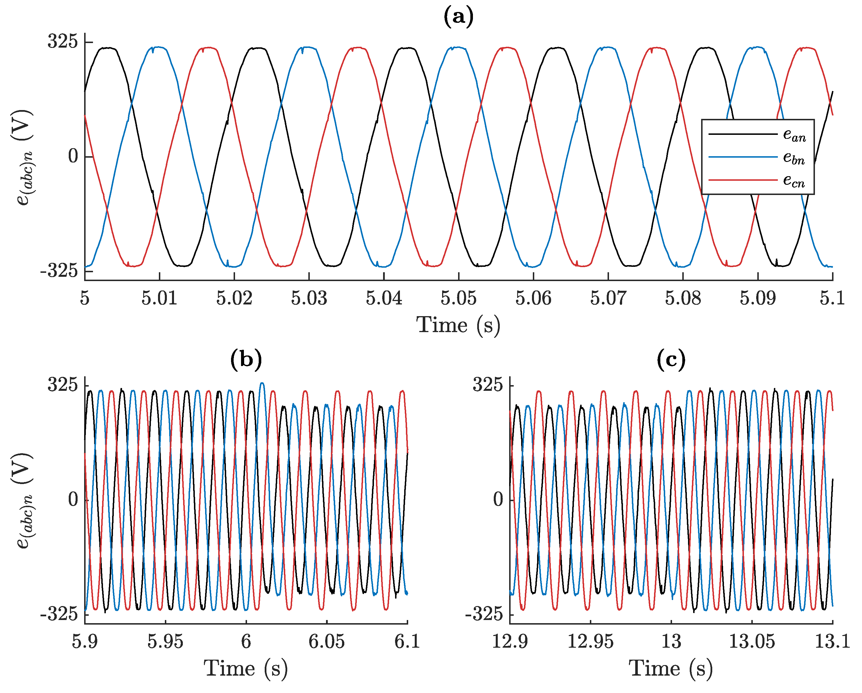
With the aim of tuning the parameters of a 2-SMC scheme commanding the GSC of a DFIG, an a posteriori MOO approach has been presented and successfully applied in this paper, both in simulation and experimentally. Two variants (i.e., design concepts) of the same 2-SMC algorithm, which only differed in the switching functions adopted, were tuned and their respective performances were compared to each other. The first algorithm contained six parameters to be tuned, while the second, whose switching functions were simplified versions of those defined for the first one, contained just four. The grid voltage was assumed to be continuously harmonically polluted, as well as subject to imbalances. In this context, the tuning process was carried out in such a way that a single set of controller parameters was valid for nine possible operating regimes of the DFIG, three of which were directly related to the appearance of imbalances in the grid voltage.

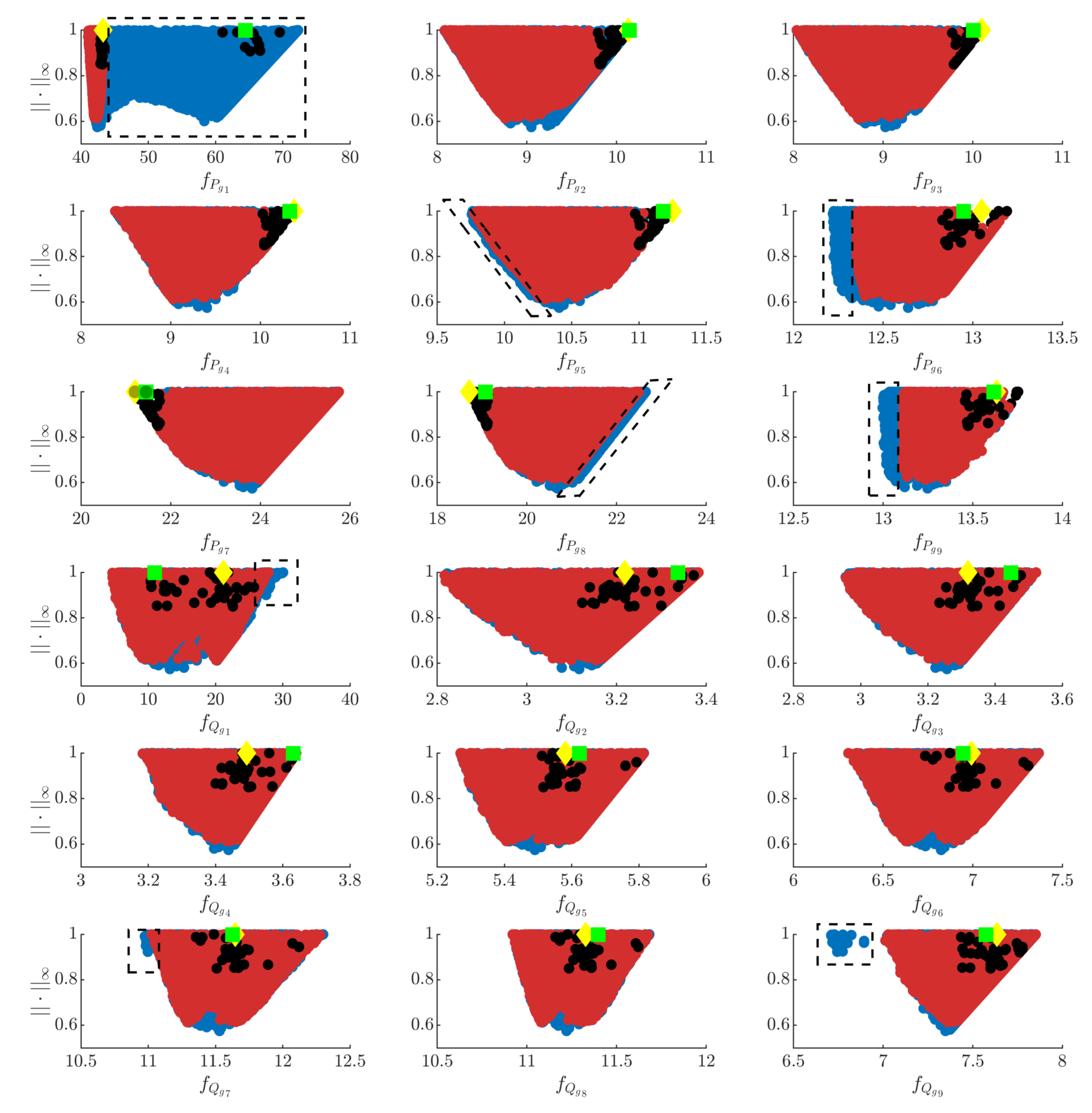
In particular, two performance indices, $f_{P_g}$ and $f_{Q_g}$, were defined for each of those nine operating regimes, which, respectively, quantify to what extent the reference values set for the grid active and reactive powers were complied with. As a result, the MOOP, on which the tuning is based, was set out by considering 18 indices in total. Driven by the high number of indices to be accounted for, the interactive tool of LDs was employed during the decision-making stage, with the purpose of facilitating analysis of the Pareto fronts (trade-off among objectives) and assisting selection of the preferred parameter sets.

The optimisation process gave rise to a Pareto front for each of the two design concepts considered. Analysis of those two Pareto fronts led to the following conclusions:

• Taking a set of experimentally validated parameters as starting point, multiple solutions to the MOO-based tuning problem were found, through simulation, by demanding that each and every one of the 18 performance indices they lead to were better than those obtained when applying the baseline parameter set.
• As expected, trade-offs among some of the $f_{{P_g}_i}$ performance indices, with $i=1,2,3\dots 9$, became evident. In contrast, the compromise between indices $f_{{P_g}_i}$ and $f_{{Q_g}_i}$ was found to be not as marked as intuitively thought beforehand.
• Although a number of solutions for the six-parameter 2-SMC algorithm behaved slightly better than those corresponding to the four-parameter variant for five of the performance indices, they also gave poorer values for another three. In summary, the six-parameter variant of the 2-SMC algorithm does not dominate that of four-parameter variant.

Considering the designer preferences, two sets of parameters (one from each design concept) were selected and compared experimentally to each other, as well as to the baseline parameter set. To that end, aiming at reducing the impact that the variability of the harmonic distortion present in the grid voltage can have on the performance indices, each of those three parameter sets underwent the same test 30 times.

A statistical analysis of the results derived from the total of 90 experimental tests carried out allows us to draw the following main conclusions:

• In good logic, it has been corroborated that the two solutions selected globally improve the performance of the parameter set adopted as a baseline solution.
• Performances comparable to those resulting from application of the six-parameter 2-SMC algorithm are achievable by using its simplified four-parameter version.

References

1. Yaramasu, V.; Wu, B.; Sen, P.C.; Kouro, S.; Narimani, M. High-power wind energy conversion systems: State-of-the-art and emerging technologies. Proc. IEEE 2015, 103, 740–788. [Google Scholar] [CrossRef]
2. Xu, L. Coordinated control of DFIG’s rotor and grid side converters during network unbalance. IEEE Trans. Power Electron. 2008, 23, 1041–1049. [Google Scholar]
3. Hu, J.; He, Y.; Xu, L.; Williams, B.W. Improved control of DFIG systems during network unbalance using PI-R current regulators. IEEE Trans. Ind. Electron. 2009, 56, 439–451. [Google Scholar] [CrossRef]
4. Xu, H.; Hu, J.; He, Y. Operation of wind-turbine-driven DFIG systems under distorted grid voltage conditions: Analysis and experimental validations. IEEE Trans. Power Electron. 2012, 27, 2354–2366. [Google Scholar] [CrossRef]
5. Sharifi, M.; Shahriari, B.; Bagheri, A. Optimization of sliding mode control for a vehicle suspension system via multi-objective genetic algorithm with uncertainty. J. Basic Appl. Sci. Res. 2012, 2, 6724–6729. [Google Scholar]
6. Mahmoodabadi, M.J.; Arabani Mostaghim, S.; Bagheri, A.; Nariman-zadeh, N. Pareto optimal design of the decoupled sliding mode controller for an inverted pendulum system and its stability simulation via Java programming. Math. Comput. Modell. 2013, 57, 1070–1082. [Google Scholar] [CrossRef]
7. Alitavoli, M.; Taherkhorsandi, M.; Mahmoodabadi, M.J.; Bagheri, A.; Miripour-Fard, A. Pareto design of sliding-mode tracking control of a biped robot with aid of an innovative particle swarm optimization. In Proceedings of the International Symposium on Innovations in Intelligent Systems and Applications, Trabzon, Turkey, 2–4 July 2012; pp. 1–5. [Google Scholar]
8. Elgammal, A.A.A.; El-naggar, M.F. MOPSO-based optimal control of shunt active power filter using a variable structure fuzzy logic sliding mode controller for hybrid (FC-PV-Wind-Battery) energy utilisation scheme. IET Renew. Power Gener. 2017, 11, 1148–1156. [Google Scholar] [CrossRef]
9. Qin, Z.C.; Xiong, F.R.; Ding, Q.; Hernández, C.; Fernandez, J.; Schütze, O.; Sun, J.Q. Multi-objective optimal design of sliding mode control with parallel simple cell mapping method. J. Vib. Control 2017, 23, 46–54. [Google Scholar] [CrossRef]
10. Trebi-Ollennu, A.; White, B.A. Multiobjective fuzzy genetic algorithm optimisation approach to nonlinear control system design. IEE Proc.-Control Theory Appl. 1997, 144, 137–142. [Google Scholar] [CrossRef]
11. Martínez, M.I.; Susperregui, A.; Tapia, G. Second-order sliding-mode-based global control scheme for wind turbine-driven DFIGs subject to unbalanced and distorted grid voltage. IET Electr. Power Appl. 2017, 11, 1013–1022. [Google Scholar] [CrossRef]
12. Mattson, C.A.; Messac, A. Pareto frontier based concept selection under uncertainty, with visualization. Optim. Eng. 2005, 6, 85–115. [Google Scholar] [CrossRef]
13. Herrero, J.M.; Reynoso-Meza, G.; Martínez, M.; Blasco, X.; Sanchis, J. A smart-distributed Pareto front using the ev-MOGA evolutionary algorithm. Int. J. Artif. Intell. Tools 2014, 23, 1450002. [Google Scholar] [CrossRef]
14. Coello, C.A.; Lamont, G.L.; van Veldhuizen, D.A. Evolutionary Algorithms for Solving Multi-Objective Problems, 2nd ed.; Genetic and Evolutionary Computation; Springer: Berlin/Heidelberg, Germany, 2007. [Google Scholar]
15. Blasco, X.; Herrero, J.M.; Sanchis, J.; Martínez, M. A new graphical visualization of n-dimensional Pareto front for decision-making in multiobjective optimization. Inf. Sci. 2008, 178, 3908–3924. [Google Scholar] [CrossRef]
16. Blasco, X.; Herrero, J.M.; Reynoso-Meza, G.; Martínez Iranzo, M.A. Interactive tool for analyzing multiobjective optimization results with level diagrams. In Proceedings of the Genetic and Evolutionary Computation Conference Companion, Berlin, Germany, 15–19 July 2017; pp. 1689–1696. [Google Scholar]
17. Huilcapi, V.; Blasco, X.; Herrero, J.M.; Reynoso-Meza, G. A loop pairing method for multivariable control systems under a multi-objective optimization approach. IEEE Access 2019, 7, 81994–82014. [Google Scholar] [CrossRef]
18. Huilcapi, V.; Lima, B.; Blasco, X.; Herrero, J.M. Optimización multiobjetivo en modelado y control de un péndulo invertido rotatorio. Rev. Iberoam. Autom. Inf. Ind. 2018, 15, 363–373. [Google Scholar] [CrossRef]
19. Boada, Y.; Reynoso-Meza, G.; Picó, J.; Vignoni, A. Multi-objective optimization framework to obtain model-based guidelines for tuning biological synthetic devices: An adaptive network case. BMC Syst. Biol. 2016, 10, 27. [Google Scholar] [CrossRef] [PubMed]
20. Beltran, B.; Benbouzid, M.E.H.; Ahmed-Ali, T. Second-order sliding mode control of a doubly fed induction generator driven wind turbine. IEEE Trans. Energy Convers. 2012, 27, 261–269. [Google Scholar] [CrossRef]
21. Vas, P. Sensorless Vector and Direct Torque Control, 1st ed.; Oxford University Press: New York, NY, USA, 1998. [Google Scholar]
22. Martinez, M.I.; Susperregui, A.; Tapia, G.; Xu, L. Sliding-mode control of a wind turbine-driven double-fed induction generator under non-ideal grid voltages. IET Renew. Power Gener. 2013, 7, 370–379. [Google Scholar] [CrossRef]
23. Rodriguez, P.; Timbus, A.V.; Teodorescu, R.; Liserre, M.; Blaabjerg, F. Flexible active power control of distributed power generation systems during grid faults. IEEE Trans. Ind. Electron. 2007, 54, 2583–2592. [Google Scholar] [CrossRef]
24. Utkin, V.; Guldner, J.; Shi, J. Sliding Mode Control in Electro-Mechanical Systems, 2nd ed.; CRC Press: Boca Raton, FL, USA, 2009. [Google Scholar]
25. Miettinen, K.M. Nonlinear Multiobjective Optimization, 1st ed.; Kluwer Academic Publishers: Boston, MA, USA, 1999. [Google Scholar]
26. Coello, C.A.; Lamont, G.B. Applications of Multi-Objective Evolutionary Algorithms, 1st ed.; World Scientific: Singapore, 2004. [Google Scholar]
27. Reynoso-Meza, G.; Blasco, X.; Sanchis, J.; Herrero, J.M. Comparison of design concepts in multi-criteria decision-making using level diagrams. Inf. Sci. 2013, 221, 124–141. [Google Scholar] [CrossRef] [Green Version]
28. Tušar, T.; Filipič, B. Visualization of Pareto front approximations in evolutionary multiobjective optimization: A critical review and the prosection method. IEEE Trans. Evol. Comput. 2015, 19, 225–245. [Google Scholar] [CrossRef]
29. Reynoso, G.; Blasco, X.; Sanchis, J.; Herrero, J.M. Controller Tuning with Evolutionary Multiobjective Optimization: A Holistic Multiobjective Optimization Design Procedure, 1st ed.; Springer International Publishing AG: Gewerbestrasse, Switzerland, 2017. [Google Scholar]
30. Pajares, A.; Blasco, X.; Herrero, J.M.; Reynoso-Meza, G. A new point of view in multivariable controller tuning under multiobjetive optimization by considering nearly optimal solutions. IEEE Access 2019, 7, 66435–66452. [Google Scholar] [CrossRef]
31. Herrero, J.M. Identificación Robusta de Sistemas no Lineales mediante Algoritmos Evolutivos. Ph.D. Thesis, Universitat Politècnica de València, València, Spain, October 2006. [Google Scholar]
32. López, J.; Gubía, E.; Sanchis, P.; Roboam, X.; Marroyo, L. Wind turbines based on doubly-fed induction generator under asymmetrical voltage dips. IEEE Trans. Energy Convers. 2008, 23, 321–330. [Google Scholar] [CrossRef]
Figure 1. Structure of a doubly-fed induction generator (DFIG)-based wind turbine.
Energies 12 03782 g001
Figure 2. Functional diagram of the control scheme adopted for a DFIG grid-side converter (GSC).
Energies 12 03782 g002
Figure 3. Scheme of the GSC and L-type grid filter.
Energies 12 03782 g003
Figure 4. (a) Pareto front f ( X p ) for a bi-objective multi-objective optimisation problem (MOOP); and (b) the Pareto set X p in the decision space. f ( X p * ) and X p * represent a possible characterisation of f ( X p ) and X p , respectively.
Energies 12 03782 g004
Figure 5. Three design concepts in a bi-objective optimisation problem. Example of comparison in the objective space.
Energies 12 03782 g005
Figure 6. Comparison of design concepts 1, 2, and 3 by employing level diagrams (LDs) with the Euclidean norm. (a) LD graph for objective f 1 ; and (b) LD graph for objective f 2 .
Energies 12 03782 g006
Figure 7. Grid voltage profile: (a) Harmonic distortion in the absence of imbalance; (b) zoom at the start of the imbalance; and (c) zoom at the end of the imbalance.
Energies 12 03782 g007
Figure 8. Profiles for P r and P g o s c * throughout the test: (a) P r ; (b) P g o s c * ; (c) detail of P r at the steady state of the imbalance; and (d) detail of P g o s c * at the steady state of the imbalance.
Energies 12 03782 g008
Figure 9. Comparison of Pareto fronts by means of LDs with the -norm. Blue and red dots correspond to design concepts 1 ( f ( X p * C 1 6 p ) ) and 2 ( f ( X p * C 2 4 p ) ), respectively. Dashed lines delimit regions where differences between the two design concepts become more evident. Black dots denote solutions selected to illustrate the trade-off existing among the values of the objectives. The green square and yellow diamond mark, respectively, the preferred six-parameter ( f ( x C 1 6 p , A ) ) and four-parameter ( f ( x C 2 4 p , B ) ) solutions.
Energies 12 03782 g009
Figure 10. Pareto set of design concept 1 ( X p * C 1 6 p ) resulting from application of LD with -norm. Black dots correspond to solutions selected to illustrate the trade-off among objectives. The green square marks the preferred six-parameter solution, x C 1 6 p , A .
Energies 12 03782 g010
Figure 11. Pareto set of design concept 2 ( X p * C 2 4 p ) resulting from application of LD with -norm. Black dots correspond to solutions selected to illustrate the trade-off among objectives. The yellow diamond marks the preferred four-parameter solution, x C 2 4 p , B .
Energies 12 03782 g011
Figure 12. Experimental rig: (a) Connection diagram; (b) snapshot of the test bench containing the 7 kW DFIG prototype; and (c) controlled two-phase imbalance generator.
Energies 12 03782 g012
Figure 13. Comparison, for each performance index, of the boxplots representing the data points collected experimentally for the three parameter sets assessed.
Energies 12 03782 g013