Earth Fault Location Using Negative Sequence Currents

Abstract

In this paper, a new method for locating single-phase earth faults on non-effectively earthed medium voltage distribution networks is proposed. The method requires only current measurements and is based on the analysis of the negative sequence components of the currents measured at secondary substations along medium voltage (MV) distribution feeders. The theory behind the proposed method is discussed in depth. The proposed method is examined by simulations, which are carried out for different types of networks. The results validate the effectiveness of the method in locating single-phase earth faults. In addition, some aspects of practical implementation are discussed. A brief comparative analysis is conducted between the behaviors of negative and zero sequence currents along a faulty feeder. The results reveal a considerably higher stability level of the negative sequence current over that of the zero sequence current.

1. Introduction

Feeder automation is one of the distinguishing features of smart grids. It aims at developing self-healing systems, able to locate faults and perform isolation and supply restoration automatically. Reliable fault location and indication is the key to this functionality. For short circuit faults, there are established methods for locating them, whereas, for locating earth faults, there is not a universally accepted, reliable and cost-effective method in the market for isolated neutral or compensated networks. However, a number of methods have been put forward to address this matter. A comprehensive review of the state-of-the-art methods for locating single-phase earth faults in medium voltage (MV) distribution networks is provided in Reference [1].

There are different types of fault location methods. Impedance-based methods [2,3,4,5,6,7] work based on calculating the apparent impedance seen when looking into the line from an end (measuring point) during the fault condition [8]. Since the line length between the measuring point and the fault location is proportional to the calculated impedance, by knowing the line impedance per unit length, the fault distance can be estimated. In Reference [2], the fault location and resistance are estimated using an iterative method. In Reference [3], a model developed for high-impedance faults consisting of two antiparallel diodes is proposed. A parameter estimation procedure is performed which uses the proposed model along with voltage and current signals to estimate the fault distance and other parameters. In Reference [4], the whole load of the feeder is modelled as one equivalent load tap located where the voltage drop due to the fault is at a maximum. Two assumptions are made i.e., once the load tap is assumed to be located before the fault point and once it is assumed to be after the fault. By solving the equations corresponding to those assumptions, the fault distance is estimated in unearthed networks. The method presented in Reference [5] scans the data obtained from power quality monitors and relays to estimate the fault distance in terms of the line impedance. The concept introduced in Reference [4] can be adapted for compensated distribution networks as presented in Reference [6]. In Reference [7], a method for fault distance calculation for compensated networks is put forward which requires a fewer number of settings compared to the method presented in Reference [4]. Despite all the efforts, these impedance-based methods are subject to errors as the fault impedance is unknown. Moreover, to locate single-phase to ground faults, the phase to ground voltages must be available [4], which is cost prohibitive. Generally, these methods are more suitable in transmission lines.

Travelling-wave based methods [9,10,11,12,13] work based on the transient voltages and currents (impulses) which are generated at the fault location. These waves propagate away from the fault point in both directions towards the ends. As these types of waves travel at the speed of light, by measuring the wave and their reflection arrival times at either terminal of the line, the fault distance can be determined [8]. A concept to create travelling waves is proposed in Reference [9], which is based on earthing the neutral via a controlled thyristor that provides a short period of high fault current. The method in Reference [10] works based on frequency spectrum components of waves generated as a result of fault occurrence. Reference [11] is based on the wave velocity of zero and aerial mode components and their arriving timestamps. Some results from field tests are reported in Reference [12] indicating the limitations of applying travelling wave fault location on distribution networks. In Reference [13], the frequency information of travelling voltage waves is integrated with their time domain information using continuous wavelet transform to locate faults. However, the main problem when using travelling-wave based methods is that due to the large number of branches and laterals in distribution networks, the reflections captured at the beginning of the feeder, may come from different sources and not necessarily from the fault location only. This makes the use of traveling wave-based methods problematic in distribution networks.

Signal injection-based methods are another type of fault location method [14,15,16]. The idea is to inject a pulsating current into the neutral of the system following a fault occurrence. The injected signal is detectable only in the faulted feeder and from the injection point up to the fault point. Although, this method has been field tested, the results show that it can be used for fault resistances only up to 300 Ω (without voltage measurement). In addition, the use of this method is limited to only compensated networks where the injection device can be coupled with the Petersen coil.

In References [17,18,19,20], earth fault location using zero sequence components is proposed. Despite the simplicity this approach offers, it suffers from a shortcoming i.e., false indication in networks where the length of the faulty feeder is long and the fault occurs close to the beginning of the feeder. In addition, this method in the manner proposed in Reference [20], when applied to compensated networks, requires connection and disconnection of the resistor in parallel with the Petersen coil in the right time, which could cause complexity.

Despite all these efforts, earth fault location in isolated and compensated neutral distribution networks remains a problem for which there does not seem to be a widely adopted solution and thus it is worth studying. Fault indication and location is a more challenging task in isolated and compensated neutral networks because their fault currents are so low that the simple threshold detection will often lead to poor results. One solution is to utilize neutral voltage measurement, in addition to current measurement. However, this neutral voltage measurement is not usually preferred at the MV side due to additional costs [18]. Therefore, there is a need for an earth fault indication method which is based on current measurement only. On the other hand, recent developments in smart grids have enabled communication between different parts of the network. By taking advantage of this feature, better solutions can be achieved as measurements from different parts of the network can be utilized to locate the fault.

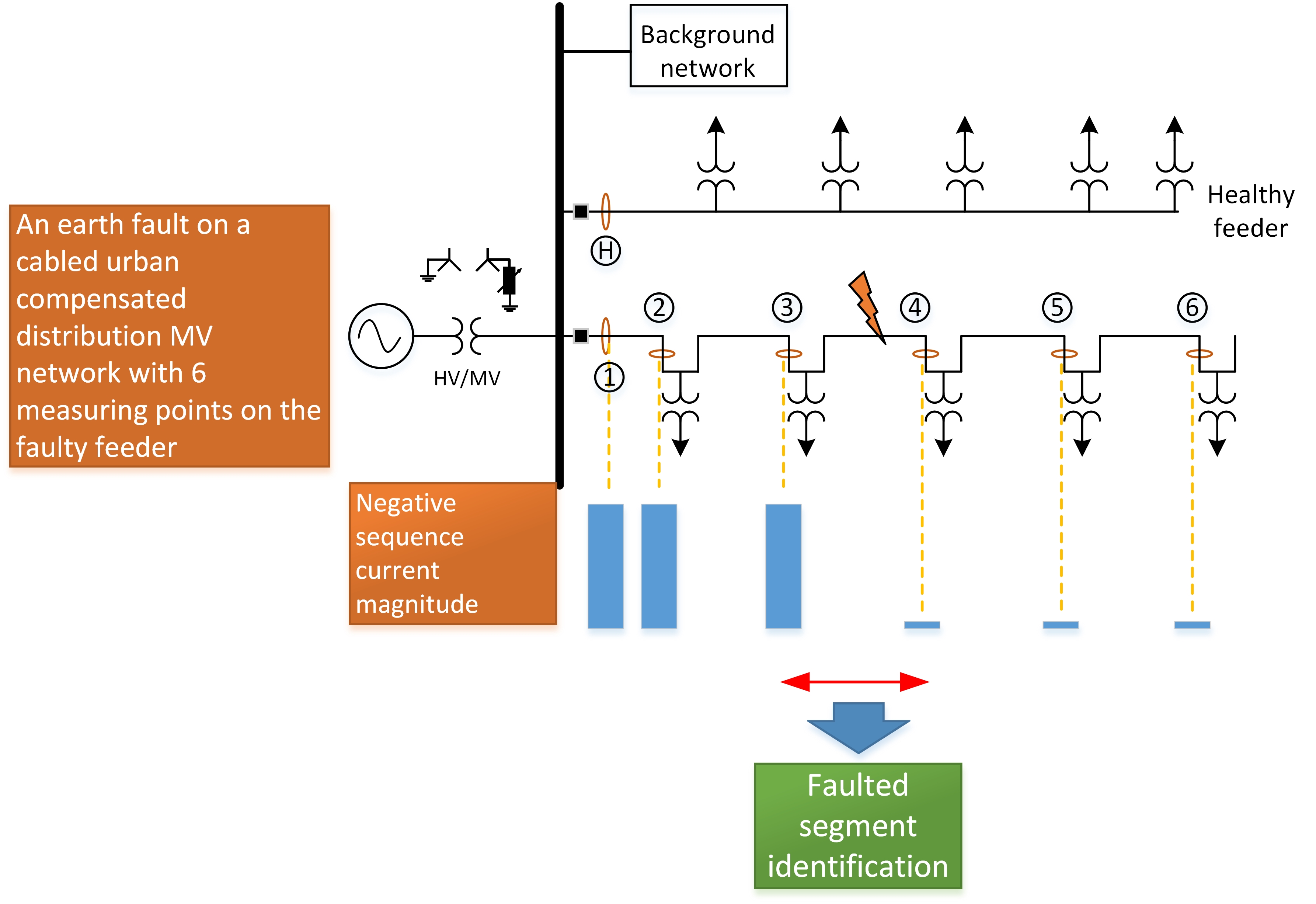
In this paper, a new method for identifying the faulted segment (the segment between two secondary substations on which fault has occurred) in case of a single-phase to ground fault is presented. It is purely based on current measurements and no voltage measurement is required, which can be considered as an advantage. The proposed method employs the negative sequence current components to locate the fault. First, In Section 2, the negative sequence current along a faulted feeder is analysed in depth to gain insights into its behaviour. Then, based on that analysis, the fault location procedure is established in Section 3. In Section 4, the effectiveness of the method is evaluated by means of simulation using various types of medium voltage distribution networks. Lastly, some aspects of implementing the proposed method are discussed in Section 5.

2. Theoretical Background of the Proposed Method

In this section, to gain some insight into the proposed fault location method, the negative sequence currents on different locations on a feeder following a fault occurrence are discussed. The focus is on the difference between the negative sequence currents before and after the fault point.

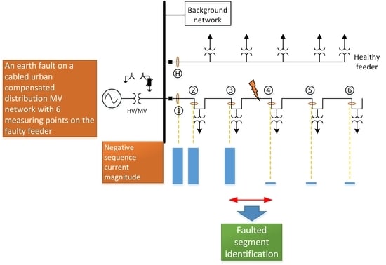
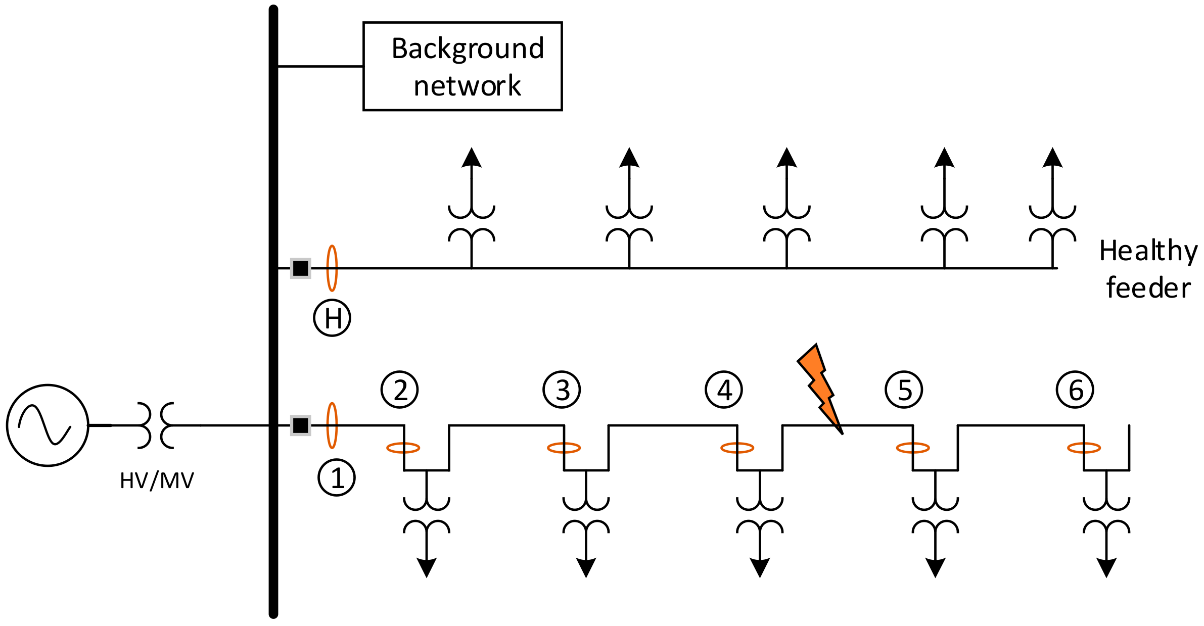
To have a better understanding of the fault current, an MV distribution network with one healthy feeder and one with a single-phase to ground fault on it is shown in Figure 1. Earth capacitances and the flow of currents following a fault occurrence are shown in the figure. Fault current, especially in isolated neutral networks, is determined by network capacitances and mostly by the undamaged parts of the network.

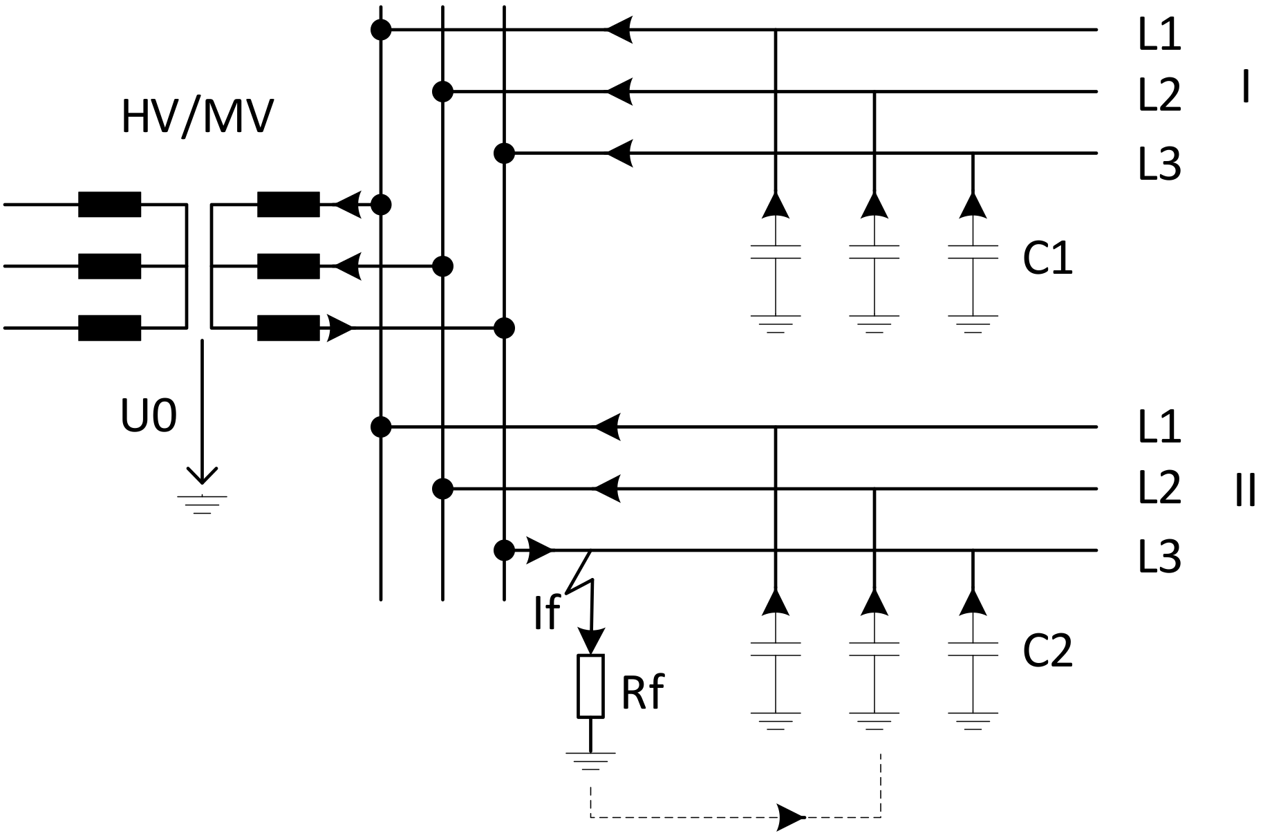
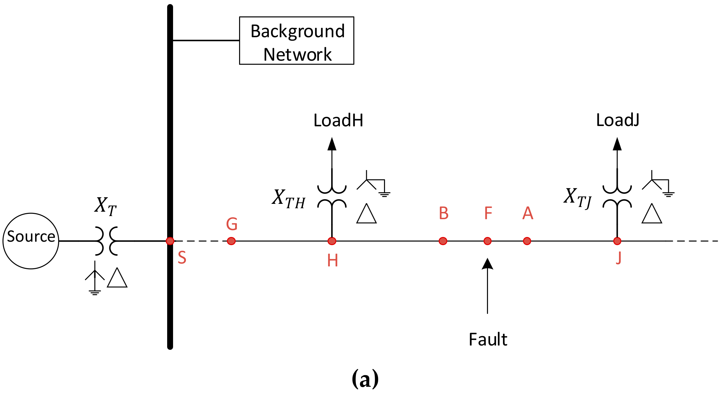
For studying the fault location problem with more details, the MV distribution network shown in Figure 2 is used. In this paper, the style of single line diagrams is derived from Reference [22]. A typical MV network consists of several feeders but from a theoretical viewpoint, only the faulty feeder needs to be studied with more details and others can be represented by a simple electrical equivalent circuit This aspect is considered in the figure using the single block “Background network” representing all the healthy feeders. A single-phase to ground fault occurs on the feeder under study between two secondary substations H and J at point F with the fault resistance $R_F$. The dashed lines indicate that the feeder can be of any length and can have any number of secondary substations. 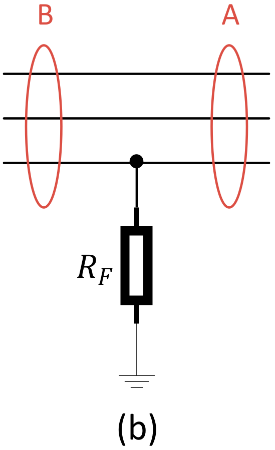In Figure 2a, two arbitrary secondary substations are shown which indicates that the following analysis is valid for any point on the feeder. The goal here is to analyse the negative sequence current at point B, which is before the fault point and the negative sequence current after the fault location at point A. Note that points B and A are not electrically the same location. This is shown, for clarification, in Figure 2b.

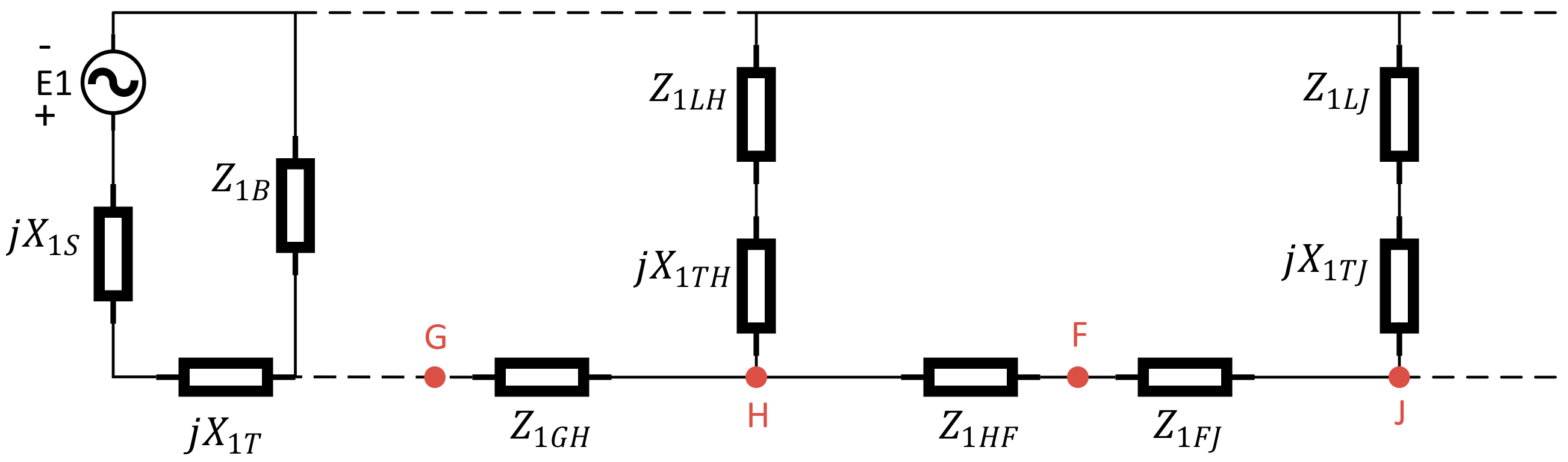
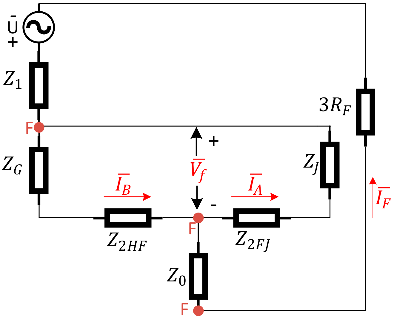
The sequence equivalent networks of the MV distribution system shown in Figure 2 can be obtained, as shown in Figure 3, Figure 4 and Figure 5 (see also the notations list presented at the beginning of the paper). Note that line (to earth) capacitances only appear in the zero sequence network. In case of a single phase to ground fault, the sequence networks will be connected in series. The complete sequence network of the faulted network under study is shown in Figure 6. It can be simplified, as shown in Figure 7 where $Z_G$ and $Z_J$ are equivalent impedances of the parts marked on Figure 6. The currents $\overline{I_B}$ and $\overline{I_A}$ are the fundamental frequency components of the negative sequence currents at points B (before the fault) and A (after the fault) in Figure 2, respectively.

The values of load impedances are normally rather large compared to the system impedances, so that they have a negligible effect on the faulted phase current. Therefore, it is common practice in fault analysis to neglect load impedances for shunt faults [22]. However, in the following, both scenarios are discussed, i.e., one where the effect of load is neglected and another where its effect is considered.

2.1. With No Load

Consider Figure 6. Shunt branches consist of transformers’ reactance in series with load impedances. With no load assumption, the values of all the load impedances in the shunt branches are infinite and hence no current flows through the shunt branches in the positive and negative sequence networks. As a result, the negative sequence current measured at any point from beginning of the feeder to the fault point is constant and it is zero after the fault point. Therefore:

$$I_B>I_A$$

(1)

where, $I_B$ and $I_A$ are the magnitudes of the phasors $\overline{I_B}$ and $\overline{I_A}$, respectively.

2.2. With Load

In Figure 6, when taking load impedances into account, the negative sequence current measured along the feeder from S to F is not constant anymore as some currents will flow through the shunt branches as well. In addition, similarly, due to the flow of current through shunt branches after the fault point, the negative sequence current after the fault point is not zero anymore.

In practice, the series impedances in Figure 6 are negligible when compared to the shunt impedances, with the exception of $Z_{2B}$ and $X_{2s}$. Indeed, $Z_{2B}$ is comparatively low as it is the equivalent negative sequence impedance of several feeders i.e., the background network.

Now, consider Figure 7 which shows the simplified network where $Z_G$ and $Z_J$ are the total negative sequence impedances before and after the fault point, respectively. In Figure 7, the following is valid.

$${\overline{I}}_B={\overline{I}}_A+{\overline{I}}_F$$

(2)

$${\overline{I}}_B=\frac{{\overline{V}}_f}{Z_G+Z_{2HF}}$$

(3)

$${\overline{I}}_A=-\frac{{\overline{V}}_f}{Z_{2FJ}+Z_J}$$

(4)

As $Z_G$ represents the part of the network which consists of negligible series impedances and the shunt branch $Z_{2B}$, it is a comparatively low impedance. In contrast, $Z_J$ is a comparatively high impedance so that:

$$abs(Z_G+Z_{2HF})<abs(Z_{2FJ}+Z_J)$$

(5)

Equations (3)–(5) yield:

$$I_B>I_A$$

(6)

Therefore, the negative sequence current before the fault point is higher than the negative sequence current after the fault point in both scenarios i.e., with and without considering the load.

3. Outline of the Implementation of the Method

Considering the theory discussed in the previous section, when a single-phase-to-ground fault occurs, the negative sequence current exists and varies only a little in the section between the primary substation and the fault location whereas after the fault point, it is very low. This is simply illustrated in Figure 8.

Therefore, the proposed new fault location procedure is structured as follows:

• The (change in the) negative sequence current at secondary substations (ideally at every substation) is obtained, following a fault occurrence.
• These values are compared with a pre-set threshold at secondary substations.
• Only from those secondary substations in which the threshold is exceeded, the fault detection information is sent to the control room.
• The faulted segment is identified as the section between the last secondary substation that sends the fault detection information and the first secondary substation from which comes no signal.

For example, in Figure 8, the fault information is sent to the control room from those measuring points at which the magnitude of the negative sequence current has exceeded the threshold i.e., measuring points 1–4. The last three secondary substations (points 5–7) send no signal to the control room and therefore the faulted segment is identified as the one linking measuring points 4 and 5.

4. Simulation Results

To evaluate the validity of the proposed method, a set of simulations was carried out with PSCAD™/EMTDC™. The effectiveness of the proposed method was studied with different fault resistances in each of the following network types:

• Cabled urban compensated network;
• Cabled urban isolated neutral network;
• Rural compensated network;
• Rural isolated neutral network.

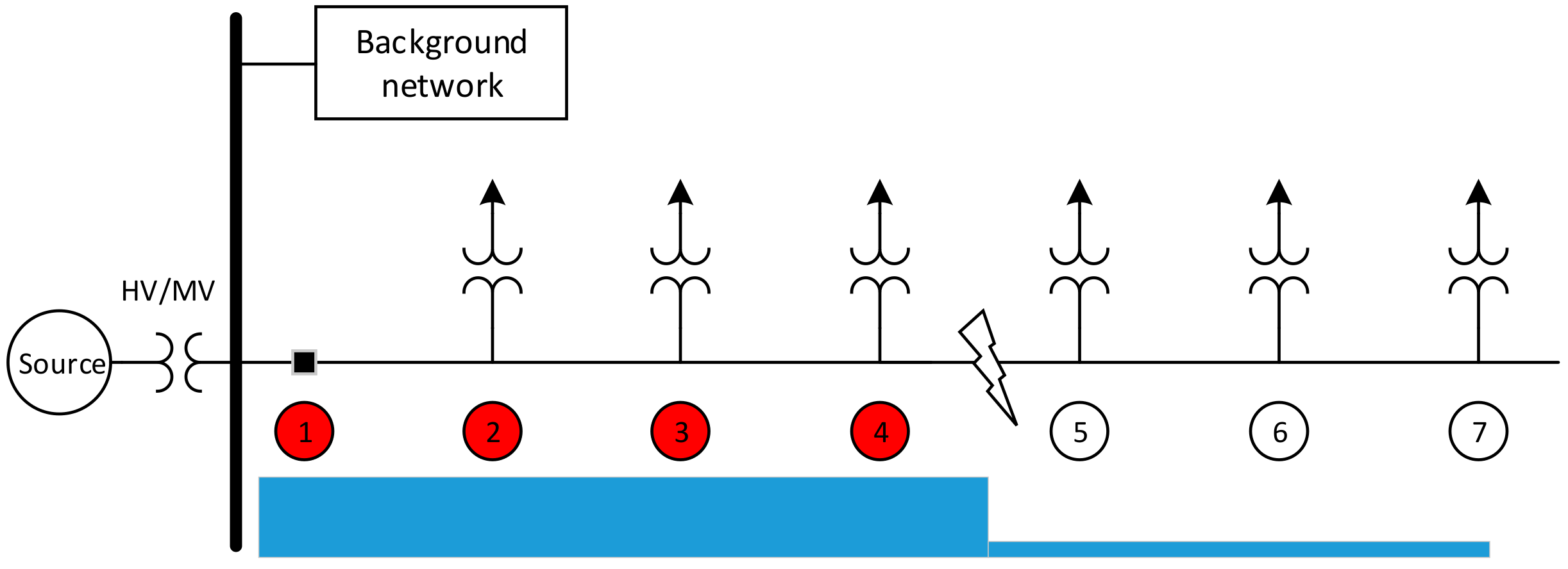
The network shown in Figure 9 is an urban compensated medium voltage distribution network with compensation degree 0.95. The voltage level in the medium voltage side is 20 kV which is fed from a 110-kV supply network using a 40 MVA transformer. The length of the feeder under study is 5.4 km consisting of AHXAMK underground cables. The feeder under study has five secondary substations equipped with current measurements. The current measurement points 2–6 are the secondary substations along the feeder, points 1 is at the beginning of the feeder and H refers to the measuring point at the beginning of an adjacent healthy feeder. A single-phase-to-earth fault, with the resistance of 30 Ω, occurs at 2.5 km from the beginning of the feeder.

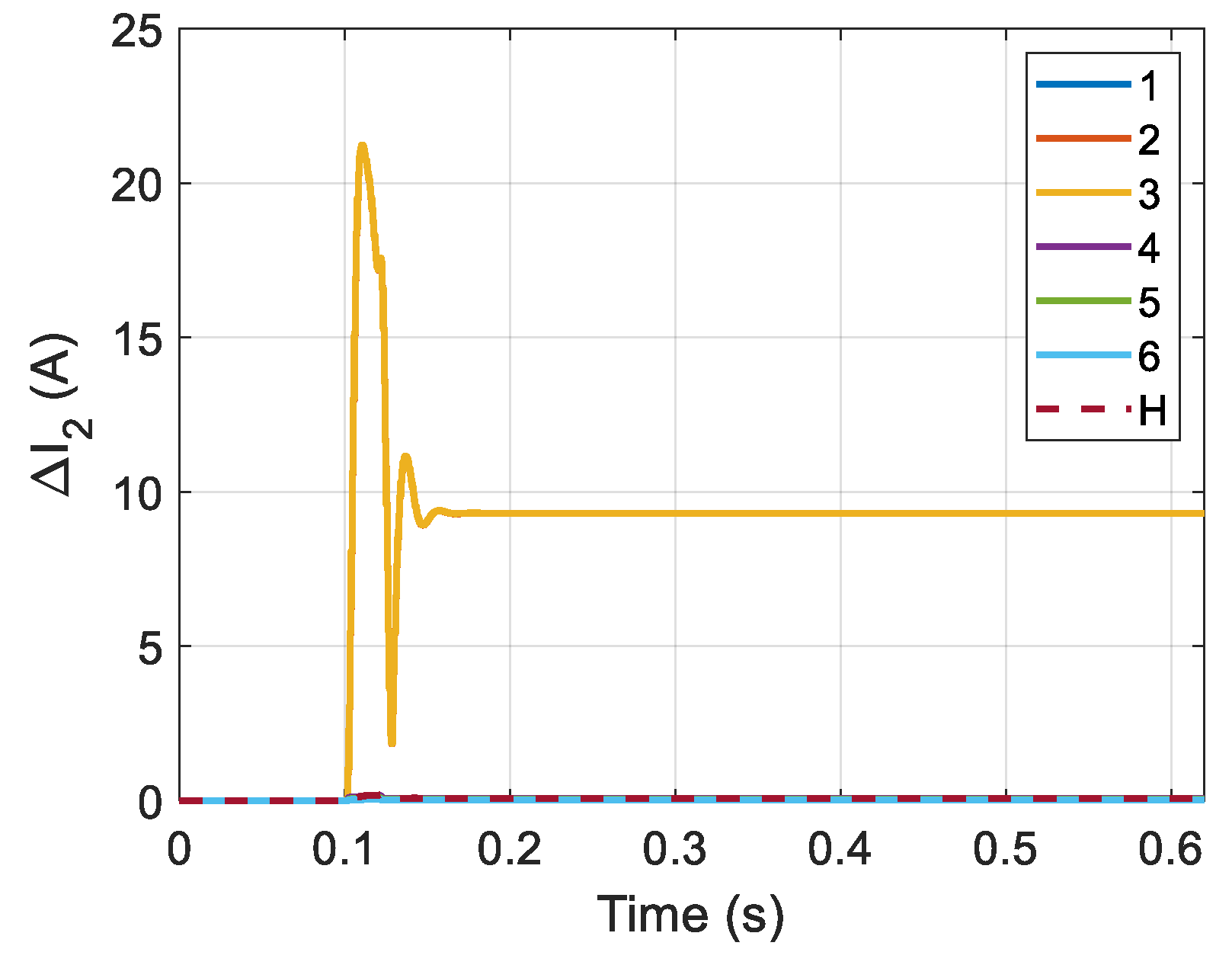
The magnitudes of the fundamental frequency phasors of the negative sequence currents with respect to time for faulty and healthy feeders are shown in Figure 10. The stabilized values obtained at $t=0.2 s$ are shown in a separate figure (Figure 11). Using the proposed method, one can readily determine the faulted section i.e., the one between secondary substations with measuring points 3 and 4. There is a considerable difference in the amplitude of the negative sequence currents before and after the fault points so that the negative sequence current is practically negligible after the fault point. It is worth noticing that the negative sequence current of the healthy feeder behaves in a similar way as that of the points after the fault point.

In addition, the variations of the negative sequence currents along the feeder from the beginning of it up to the fault point are so insignificant that the first three graphs (corresponding to locations before the fault point) are almost matched. This highlights the strength of using the negative sequence current in locating faults.

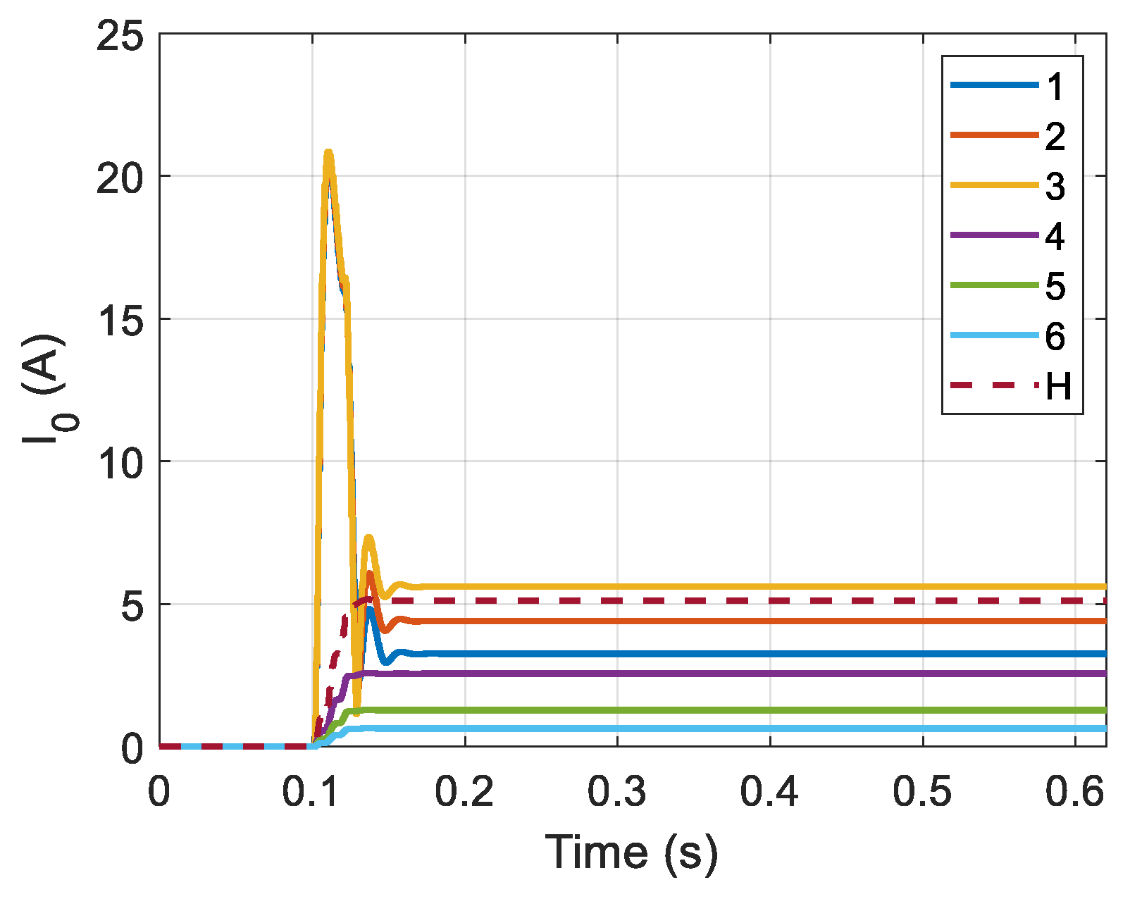
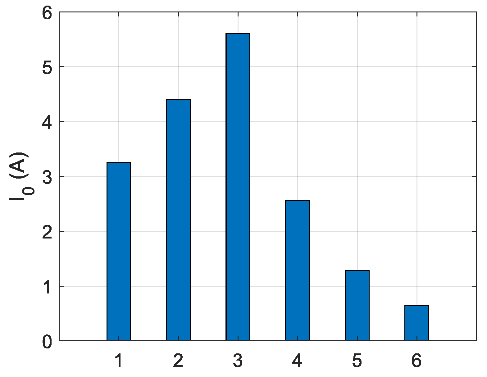
To enable a comparison between negative and zero sequence currents, similar types of graphs are obtained for the zero sequence currents and shown in Figure 12 and Figure 13. Contrary to the negative sequence current, the zero-sequence current varies considerably along the feeder and is not negligible after the fault point. This reveals the shortcoming of using the zero-sequence current over the negative sequence current.

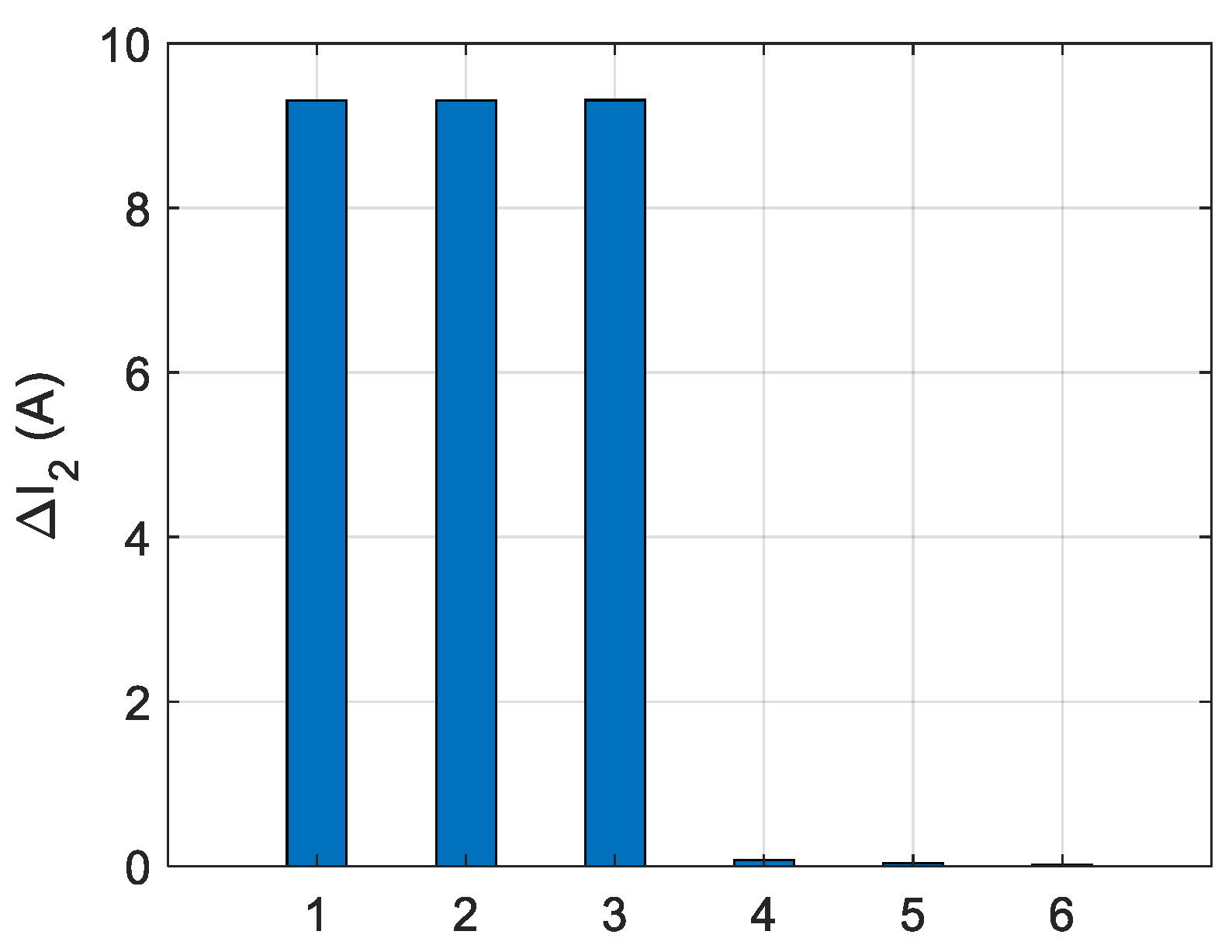
To further investigate the validity and performance of the proposed method, five fault resistances are studied ranging from 0.01 Ω up to 1 kΩ. The changes in the negative sequence currents, caused by the fault, at the beginning of the healthy and faulty feeders and at each secondary substation of the faulty feeder are provided in

Table 1. Negative sequence currents in urban compensated network.

Rf (Ω)	∆In1 (A)	∆In2 (A)	∆In3 (A)	∆In4 (A)	∆In5 (A)	∆In6 (A)	∆InH (A)
0.01	9.57	9.57	9.57	2.6	0.04	0.02	0.08
1	9.48	9.48	9.49	2.6	0.04	0.02	0.08
10	9.41	9.41	9.41	2.59	0.04	0.02	0.08
100	8.81	8.81	8.82	2.42	0.03	0.02	0.07
1000	3.38	3.37	3.38	0.92	0.01	0.01	0.03

. The choice of the threshold might vary from network to network. Developing a procedure to decide the proper threshold for a given network is not the focus of this paper. For simulations presented in this paper, the threshold is chosen to be 3 A for urban networks and 2 A for rural networks. For fault resistances between 0.01 Ω and 1000 Ω, it is clear from the table that for points 1 to 3, negative sequence currents exceed the threshold (3 A) whereas these values are below the threshold for points 4 to 6. Therefore, the faulted segment is the one between the second and third secondary substations i.e., between points 3 and 4.

The same procedure can be applied to isolated networks, as shown in Figure 14. The changes in the negative sequence currents, following the fault occurrence, are provided in

Table 2. Negative sequence currents in urban isolated network.

Rf (Ω)	∆In1 (A)	∆In2 (A)	∆In3 (A)	∆In4 (A)	∆In5 (A)	∆In6 (A)	∆InH (A)
0.01	58.91	58.9	58.94	56.54	0.26	0.13	0.48
1	58.89	58.88	58.92	56.51	0.26	0.13	0.48
10	58.06	58.06	58.09	55.72	0.25	0.13	0.48
100	31.73	31.73	31.75	30.45	0.14	0.07	0.26
1000	3.85	3.85	3.85	3.68	0.02	0.01	0.03

. Using the table and the same 3 A threshold, the faulted segment can be determined successfully for all the 5 fault resistances.

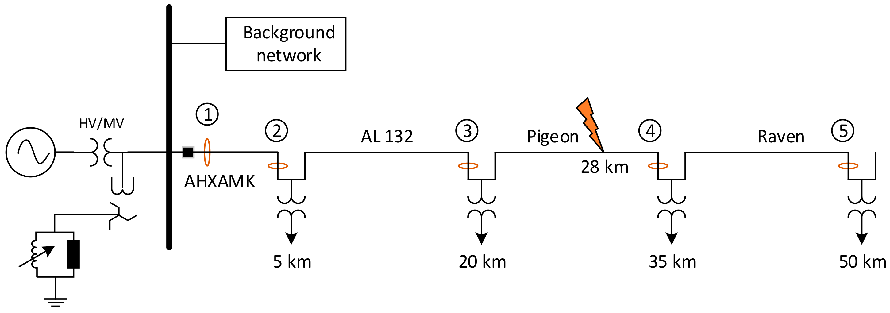
Now consider the rural compensated network shown in Figure 15. The first 5 km of the feeder under study consists of cables and the rest 45 km is overhead lines. The cable and overhead lines types modelled in the simulations are shown on the figure. A single-phase to ground occurs at 28 km from the beginning of the feeder. Similarly, using a threshold of 2 A and

Table 3. Negative sequence currents in rural compensated network.

Rf (Ω)	$\mathbf{\Delta }$ln1 (A)	$\mathbf{\Delta }$ln2 (A)	$\mathbf{\Delta }$ln3 (A)	$\mathbf{\Delta }$ln4 (A)	$\mathbf{\Delta }$ln5 (A)
0.01	5.25	5.25	5.26	0.59	0.29
1	5.25	5.24	5.26	0.59	0.29
10	5.21	5.21	5.22	0.59	0.29
100	4.94	4.94	4.95	0.56	0.27
1000	2.39	2.38	2.39	0.27	0.13

, the faulted segment is successfully identified, as the one between the second and third secondary substations (points 3 and 4).

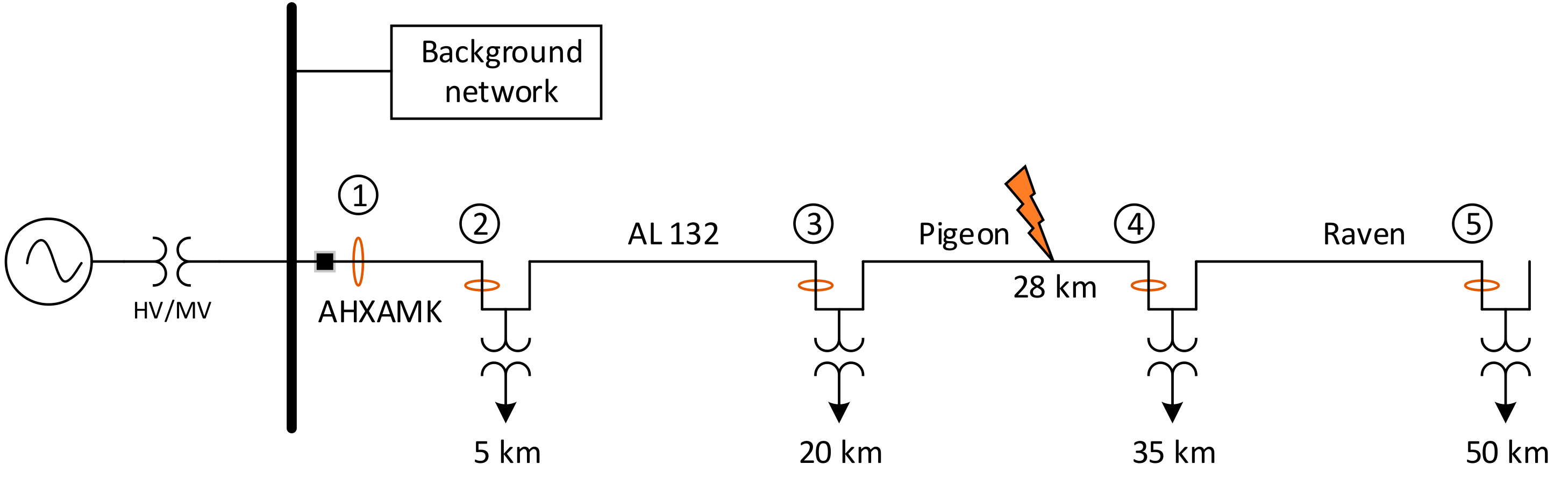
Lastly, in Figure 16, a rural isolated neutral network is shown. The change in the magnitude of the negative sequence currents for the points marked on the figure are shown in

Table 4. Negative sequence currents in rural isolated network.

Rf (Ω)	$\mathbf{\Delta }$ln1 (A)	$\mathbf{\Delta }$ln2 (A)	$\mathbf{\Delta }$ln3 (A)	$\mathbf{\Delta }$ln4 (A)	$\mathbf{\Delta }$ln5 (A)
0.01	15.21	15.19	15.23	1.72	0.85
1	15.21	15.19	15.23	1.72	0.85
10	15.16	15.13	15.18	1.72	0.84
100	13.4	13.37	13.41	1.52	0.74
1000	3	3	3.01	0.34	0.17

. In a similar fashion, the faulted segment is determined as the one between points 3 and 4 using the same 2 A threshold.

5. Discussion

In practice, current measurements at each secondary substation can be made using Rogowski coils, which are also suitable for retrofit installations. In the tables presented in Section 4, there are current values which are very low. It should be noted that the accuracy of the negative sequence current depends on the accuracy of CTs or current sensors (Rogowski coils) used and that decides the lowest possible value of the negative sequence current that can be reliably measured.

When a fault occurs on a distribution feeder, the information on the fault conditions must be delivered to the control room where SCADA system or DMS processes the information to visualize the fault location to the operator or to generate an automatic FLIR (fault location, isolation and restoration) switching sequence. The proposed method requires some level of communication between secondary substations and the primary substation. However, as communication will be widespread in future distribution networks, the proposed method is worth considering.

In an ideal symmetrical network, the negative zero sequence measured at any point is zero under normal condition. However, in practice, there is some level of negative sequence current even under no fault condition, for example due to asymmetry of loads. Therefore, it is important to note that the proposed method is based on the change in the negative sequence current and not the negative sequence current alone.

Compared to the current injection method presented in Reference [14], the proposed method in this paper has a clear advantage as there is no need for any extra injecting device. In addition, the pulse injection method works only with compensated neutral networks where the injection device can be connected in parallel with the Petersen coil. For isolated neutral networks where there is no possibility for connecting the injection device, the pulse injection method cannot be used.

In case of a single-phase-to-ground fault, unlike the zero sequence current, the negative sequence current remains almost constant with negligible variations along the feeder as shown in Section 4. Moreover, in compensated networks, the difference in the zero sequence current level for points before and after the fault could be too low for finding suitable and reliable criteria for locating the fault. Therefore, there is a need to increase this deference level somehow. Reference [20] suggests to connect and control an additional resistor in parallel with the Petersen coil. However, that action may lead to more complexity when it comes to practical implementation. In addition, there is a risk that in case of a long feeder, the line to ground capacitances of that part of the feeder, which is located after the fault point, provide a considerable amount of zero sequence current so that the zero-sequence based method fails to operate. This highlights the advantage of using the negative sequence current over the zero sequence current in locating faults in distribution networks.

In summary, the main advantages the negative sequence current based method offers are:

• No voltage measurement is required;
• Applicable to both isolated and compensated distribution networks;
• No need for any additional injection device or resistance.

6. Conclusions

Earth fault location on MV distribution networks using the negative sequence currents in the manner proposed in this paper appears to be promising. The proposed method is applicable to both compensated and isolated neutral networks. When using this method, only current measurements are required and not voltage measurements, which is an advantage. The theoretical reasoning to justify the proposed method was discussed in detail and simulation results obtained from different types of practical MV distribution networks confirmed the validity and performance of the method. Some further studies are still needed to address the aspects relating to practical implementation and for example the effects of decentralized compensation.