Abstract
The need for efficient electrical energy consumption has greatly expanded in the process industries. In this paper, efforts are made to recognize the electrical energy consumption in a two-echelon supply chain model with a stochastic lead-time demand and imperfect production, while considering the distribution free approach. The initial investments are made for quality improvement and setup cost reduction, which ultimately reduce electrical energy consumption. The inspection costs are considered in order to ensure the good qualities of the product. Centralized and decentralized strategies are used to analyze the proposed supply chain model. The main objective of this study is to reduce the overall cost through efficient electrical energy consumption in supply chain management by optimizing the lot size, the number of shipments, the setup cost, and the failure rate. A quantity-based transportation discount policy is applied to reduce the expected annual costs, and a service-level constraint is incorporated for the buyer to avoid a stockout situation. The impact of the decision variables on the expected total costs is analyzed, and sensitivity analysis is carried out. The results show a significant reduction in overall cost, with quality improvement and setup cost reduction ultimately reducing electrical energy consumption.
1. Introduction
The supply chain is a complex process consisting of several parameters that need to be controlled. Among them, the few parameters that can be controlled by making some additional investments include the setup cost, lead time, and quality of the products, as shown by Sarkar and Sarkar [1]. Certain parts of the manufacturing units need to be improved with state-of-the-art technology to reduce the energy consumption and enhance the quality of the products. These parts are replaced with some additional investment for setup cost and process quality improvement. Managers seek to optimize the supply chain costs; therefore, they analyze various aspects of the supply chain management systems. In the process industries, the cost of energy consumption is usually a small portion of the overall production cost. Therefore, less attention is given to energy consumption. Among the various types of energies used in the supply chain operation, electrical energy is the most consumed. Thus, efforts are made in this model to recognize the cost associated with electrical energy consumption.
In the supply chain management literature, most of the supply chain models have considered a fixed setup cost, constant lead time, and the perfect quality of the products, as indicated by Sarkar et al. [2]. However, the manufacturing setup cost can be reduced, the process quality can be improved, and the lead time can be controlled by making smart investments in various aspects of the system. The production system moves from an in-control state to an out-of-control state due to the following reasons: persistent usage of the machinery, inadequate process control, human negligence, and mishandling during the shipment. Therefore, imperfect-quality products are manufactured with the perfect-quality products in a long-run production system. These imperfect products add some additional cost to the vendor in the shape of replacement costs for defective items, and during this long process, an enormous amount of energy is consumed. In the imperfect production process, a huge amount of energy is consumed during the inspection process, defective unit replacement, ordering time, and setup time. In such situations, with the enormous amount of energy consumption, the risk of product shortage may occur, which may lead to damage to the brand image.
A number of quality management practices have been reported in the production management literature to deal with the uncertainties in the production systems. In this course of action, Salameh and Jaber [3] extended the basic economic production quantity (EPQ) model to an imperfect production system by incorporating a full inspection of the entire lot, but there is not a single assumption in their model related to energy consumption during the production. The basic inventory model is extended to the case of an imperfect production process in several studies, and effective polices are provided for the overall system cost reduction. However, these studies did not consider efficient energy consumption in the production system [4,5,6]. Several models in this direction considered the defective rate as a constant, such as those in the research of Salameh and Jaber [3], Khan et al. [7], and Chung [8]. However, in many studies, the random defective rate is considered (see Tayyab and Sarkar [9] and Cárdenas-Barrón et al. [10]). Moreover, the emergence of philosophies such as “just-in-time” in the recent past has enabled managers to focus on the reduction of lead-time components. These components include the order preparation time, transit time, lead time of the supplier, time of delivery, and the setup time. In fact, the lead time is reduced by incurring an additional amount as the crashing cost on lead-time components. These costs include administrative costs, agile transportation, and the vendor’s process speed-up cost for the reduction in waiting time. There are several advantages of the reduction of the lead time in the form of a high service level, quick response time, and—due to the lead-time reduction—less energy being consumed. This can provide an advantage to overcome the uncertainties of product demand in a competitive environment (see Ben-Daya and Hariga Sarkar [5]).
Based on the above perspective, the objective of this study is to design an optimization model with the objective to reduce the total costs of the system while considering the imperfect production and the efficient electrical energy consumption. A two-echelon supply chain model with two strategies is developed in this study. The first model is developed based on a centralized framework, while the second model provides a decentralized approach. In the decentralized policy, the interactive decisions between the retailer and the manufacturer are based on the Stackelberg approach. The imperfect production process is considered with a variable lead time, and the buyer’s lead time is reduced by adding a crashing cost. Additional initial investments are made to improve the process quality and reduce the setup cost. These investments are used to update the technologies, which helps produce good quality products with less energy consumption; in turn, this will reduce the overall supply-chain costs. The initial investment made for quality improvement retains the production system in the in-control state, which saves energy consumption due to this state having a smaller number of production system failures than the existing one. The service-level constraint is used to meet the demand from the existing stock. The transportation discounts are allowed on a quantity basis, and the optimal lot size is determined. The distribution-free approach (Scarf [11] and Gallego and Moon [12]) is used to solve the model.
In this model, costs related to shortages are not considered for the buyers because of the high penalty costs associated with shortages. Due to the stockout situations, the buyer can face the worst situation in the form of goodwill or brand image loss, and if the shortage occurs during the production process, an enormous amount of energy is wasted to backorder. In the inventory management and operation management literature, it is suggested that the cost associated with shortages and service-level constraints have an equal impact on the overall cost of the model simultaneously. Due to the use of service-level constraint, the consumption of electrical energy reduces. Therefore, the service-level constraint is used as the replacement of shortages in the system. In the literature, the shortage cost is replaced with the condition on service level, and it is assumed that the buyer has set a certain service level in terms of the fill rate that satisfies the corresponding proportion of demand from the available stock [13,14,15,16]. Therefore, the service-level constraint sets a limit on the proportion of demand that was not met from the available stock, which should not exceed a specified value. Consequently, the buyer service level measure reflects that a certain fraction of the demand, which is satisfied regularly, is expressed by .
The basic inventory model by Harris [17] assumes that arriving goods are of perfect quality, although the supply process of goods rarely conforms to the specification. This results in the deviation in quantity or time, which leads to delay and might also negatively affect the brand image. To meet the inferior quality manifestations, many researchers relaxed the perfect supply assumption made in the basic inventory model. Considering the inventory model, Salameh and Jaber [3] analyzed the lot size with imperfect quality items and entire lot inspection. During the screening period in their model, defective items are collected (in batches), and those batches are sold in secondary markets that did not consider the cost associated with the energy consumption during the production. Cárdenas-Barrón [18] provided the corrected solution for the Salameh and Jaber [3] model. Ciavotta et al. [19] minimized the general setup cost within a two-stage production system. They organized the production in batches by considering identical jobs. A robust methodology is developed in the model of Dellino et al. [20] for an uncertain environment. They explained the classical economic ordered quantity with the robust optimization technique. However, no one has considered the amount and associated cost of energy consumption in their models.
To determine the imperfect items in the production model, Goyal and Cárdenas-Barrón [21] discussed a simple approach with optimal results compared to the Salameh and Jaber model [3]. Huang [22] proposed an extension to the Salameh and Jaber [3] model by integrating the inventory model and considering a single-supplier single-buyer integrated-inventory model with an imperfect production system along with inspection activity during the just-in-time environment. Their extension was amazing in the inventory field. However, with the passage of time and increasing competition, certain other parameters need to be recognized, as the energy cost is not much compared to other cost. Still, it possesses some value, which they did not recognize in their model. There are some other additional parameters in this model, such as the introduction of transportation discounts, lead-time reduction, and service-level constraints, which improve the process of the efficient utilization of energy. Ben-Daya and Hariga [5] developed an integrated inventory model to obtain the optimal lot size, the reorder point with imperfect items, and the number of shipments. They considered that the lead demand follows a normal distribution and depends on the lot size and the transportation delay. A vendor–buyer integrated inventory model was developed by Dey and Giri [6] considering the random lead-time demand, the product inspection, and the quality improvement with the shortages. Kim et al. [23] extended the integrated inventory model of Ben-Daya and Hariga [5], and proposed an improved way of calculating imperfect items with backorder items. Still, no one recognizes the cost associated with the electrical energy consumption in their modeling. The efficient electrical energy utilization can only be done once the importance of the energy is recognized.
The inventory model with a finite replenishment rate was developed by Sarkar [24] for the retailer considering the permissible delay-in-payments and stock dependent demand. The imperfect multi-stage lean production system is considered with a rework and random defective rate in the research of Tayyab and Sarkar [9]; however, in their model, rework is performed on the defective items. They did not consider the initial investment for quality improvement in an imperfect production system; by rework, additional costs are incurred on the products, and sometimes, rework is not possible for quality improvement. No author has thought about the cost associated with electrical energy consumption during defective product production. The increase in energy-related costs, including its demand, legislation, and its consumer’s environmental awareness in recent times has influenced the industries to consider carefully the energy consumption and the associated cost. Therefore, the recent studies related to the production model have considered the energy-related costs. Tang et al. [25] investigated the production planning problem in a stochastic environment, and considered the energy consumption costs for the steel production process. In their model, the energy consumption cost was the nonlinear function of production quantity. Gahm et al. [26] developed the energy-efficient scheduling approaches to improve the energy efficiency. Furthermore, they introduced three energy dimensions: energy supply, energy demand, and energetic coverage. Keller and Reinhart [27] considered an approach that integrated energy supply information in the enterprise resource planning system, and they had the idea of energy flexibility, energy efficiency, and industry internal and external energy supply.
Du et al. [28] and Todde et al. [29] developed the models considering energy consumption and energy analysis. In the Tomić and Schneider [30] model, the energy recovery methods were explained from the waste by applying a closed-loop energy recovery approach. Haraldsson and Johansson [31] studied the various types of the energy efficiency in a production system; however, their model did not consider the imperfect production system. Although energy is consumed throughout the production system, these energy consumption-related costs are usually low, which is why due importance is generally not given to them compared with the other production-related costs. Specially, the main gap in the existing literature is in the supply chain model, where the energy-related costs are not considered. These costs have an enormous impact on overall cost as well as environmental impact. This study initiates the use of energy consumption cost in a two-echelon supply with an imperfect production process.
Managers dealing with production decisions under uncertain conditions must know the lead-time distribution of the demand. However, it’s very challenging and time-consuming to find the accurate distribution pattern. Therefore, it’s crucial for industries and researchers to find a way of calculating the total system cost without having the data on lead-time demand distribution. To deal with this problem, Scarf [11] first introduced the distribution-free newsboy issue with a known standard deviation and mean of the lead-time demand. Gallego and Moon [12] modified the ordering rule of [11]. Scarf [11] initiated the ordering rule when the distribution of lead-time demand is not present. Gallego and Moon [12] simplified the approach developed by scarf [11]. This approach is used when distribution does not follow any pattern, but the variance and the mean of the demand are available. It was used for finding the optimal ordering quantity to maximize the profit in case of the worst possible distribution of the demand.
The distribution-free approach is used in many directions, specifically in the inventory field. To find the optimal ordering quantity and the reordering point, a distribution-free continuous review inventory model was developed by Moon and Choi [14]. The optimal ordering quantity and lead time were considered by Ouyang and Wu [13]. They introduced the lead-time crashing cost. Ouyang and Chang [32] utilized the logarithmic function of Porteus [33] for quality improvement in the imperfect production process by applying the distribution-free procedure. To reduce the setup cost and to improve the quality, Ouyang et al. [4] utilized the distribution-free approach in a lot size reorder point model with the imperfect production process. The continuous review inventory model by Ma and Qiu [16] considered the distribution-free approach with an improvement in the setup cost while considering a service-level constraint. A transportation discount was introduced by Shin et al. [34] in a review inventory model with controllable lead time and a service-level constraint. The joint replenishment model was provided by Braglia et al. [35] considering stochastic lead-time demand with backorder and lost sales, but they did not consider the efficient energy consumption and cost associated with energy.
The electrical energy consumption and the related costs in the imperfect production system have not been studied in the available supply chain management literature. The cost associated with electrical energy consumption is modeled in this paper. Nevertheless, these costs are a smaller portion of the production cost, but the energy is consumed in every supply chain operation, and there is a need to reduce the associated cost. The wastage of energy is not only a financial loss; it also damages the environment. The proposed study develops a two-echelon supply chain model with an imperfect production system and identifies the electrical energy consumption costs under a stochastic demand. To reach the global optimal solution, an improved algorithm is developed in this paper. The initial investments are made for quality improvement and setup cost reduction. The inspection process is performed at the buyer end to reduce the electrical energy consumption. The service-level constraint is considered, and the demand is met from the available stock. Transportation discounts are offered on a certain quantity to attract customers. The min–max distribution-free approach is considered in this model with a known mean and standard deviation regarding the lead-time demand. Generally, the information on lead-time demand distribution is difficult to collect. If the distribution is known, then the expected shortage amount can be determined by utilizing the identified distribution. If the lead-time distribution of the demand is not available, then the statistical procedures are used to calculate it. The distribution-free approach provides prominent results; therefore, this approach is utilized to develop the proposed model. Table 1 presents the contribution of this paper.

Table 1.
Contributions of authors.
2. Problem Definition, Notation, and Assumptions
This section consists of the problem definition, notations, and the assumptions of the model.
2.1. Problem Definition
A two-echelon supply chain model is considered with efficient energy consumption under an imperfect production process. In this model, some initial capital investments are made for the production process quality improvement and setup cost reduction. The investment, made in process quality improvement, is restricting the production process to move to the out-of-control state from the in-control state. When the production process moves to the out-of-control state, a huge amount of energy is wasted on defective products. Therefore, the initial investment is made for process quality improvement, and the setup cost reduction reduces the total cost of the supply chain with the efficient electrical energy consumption. A quantity-based transportation discount is offered to motivate buyers to increase their ordering quantity. Lead-time crashing cost is used for the buyer to reduce the lead time, which ultimately reduces the electrical energy consumption. The number of shipments and the smart lot size are optimized. The service-level constraint is used to avoid shortages, and the fraction of demand is met through the available inventory. Finally, the aim of this model is to minimize the overall supply chain costs with the recognition and minimum electrical energy consumption. The production lot, reorder point, and the number of shipments is optimized. The flow of the supply chain with costs associated to the vendors and buyers are shown in Figure 1.
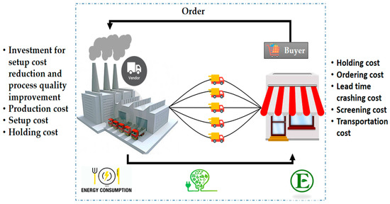
Figure 1.
Supply chain flow diagram under efficient energy consumption.
2.2. Notation
This section describes the related notation of this model (Table 2).
Table 2.
Notation for parameter and decision variables.
2.3. Assumptions
The following assumptions are considered during the formulation of the proposed supply chain management model:
- In this supply chain model, the cost of electrical energy consumed during the entire operations (e.g., during setup, ordering, inspection, and inventory holding time) is considered for a single type of product.
- The electrical energy consumption is taken care of thoroughly with continuous review of the buyer’s inventory; when the inventory level falls to the reorder point, the replenishments are made.
- When the buyer receives the lot, it is assumed that the complete lot is inspected with the screening rate under efficient electrical energy consumption. Furthermore, the assumption is made that the inspection process is non-destructive and error-free in nature.
- To omit the shortages from the model, a service-level constraint is utilized with a specific fill rate.
- The initial capital investments are made for process quality improvement and setup cost reduction by which advanced equipment can be used that consumes the minimum amount of electrical energy.
- To avoid the extra cost of electrical energy incurred due to the shortages, the supplier production rate and the screening rate are higher than the demand rate. The assumption indicates that which can be simplified as (refer to Salameh and Jaber [3]). Figure 2 shows the flow of inventory in relation to inspection time.
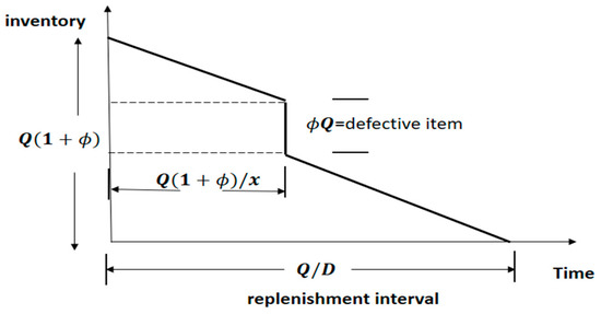 Figure 2. Inventory flow diagram.
3. Mathematical Model
The proposed mathematical model is formulated in this section for a two-echelon supply chain under energy consumption consideration.
3.1. Vendor’s Model
This section formulates the vendor’s inventory model as in the Ben-Daya and Hariga [5] model while considering the energy consumption cost in the supply chain. As in most of the supply chain models, the energy consumption cost is not considered during the process, because it is usually a small portion of supply chain cost. Nevertheless, the energy cost has a certain impact on the overall cost. The energy is consumed during various operations such as heating, cooling, lightening, etc. In this model, the electrical energy consumption is considered throughout the entire supply chain. The vendor expected annual cost comprises production setup cost with electrical energy consumption during setup time, the inventory-holding cost with electrical energy consumption, the defective unit replacement cost with energy consumption, the initial investment for setup cost reduction, and process quality improvement. This model is developed for the vendor’s production situation where the buyer places the order, and the vendor starts producing the ordered quantity until the production run has been completed. As under the single-setup multi-delivery policy, the vendor produces the items in the quantity of , and the buyer receives these products in lots of size . Therefore, the production cycle length of the vendor is .
To reduce the supply chain cost, in this model, two initial capital investments are used for product quality improvement and setup cost reduction. The concept of Porteus [33] is considered to improve the production process quality. Initially, the production process is considered as the in-control state; with the passage of time, the production process may move to the out-of-control state, where the defective units are produced until the entire lot is produced, which consumes a significant amount of energy. One good strategy that can resist the system from moving to the out-of-control state from the in-control state is an additional capital investment, which is able to reduce the energy consumptions due to the failure of the production system. For instance, to reduce the out-of-control system probability from 0.00002 to 0.000018, an investment of $200 is made; then, another $200 is furtherly required to reduce it down to 0.000016, and so on. Ultimately, making an initial investment a good choice for the reduction of imperfect production.
Production setup cost with electrical energy consumptions cost
The vendor’s setup cost per production setup is S; as under the single-setup multi-delivery policy, the vendor’s production cycle length is . A certain amount of energy is consumed during the production setup time, the energy cost incurred during setup is per setup. Therefore, the vendor’s production setup cost is:
Warranty cost with electrical energy consumptions cost
In this model, the defective units are replaced with the cost of per product and energy consumed during the defective unit replacement, and the vendor’s production cycle length is ; therefore, the annual cost of defective unit replacement is:
Process quality improvement with electrical energy consumptions cost
The capital investment ) is made (as Porteus [33]) to improve the process quality with a reduction in the out-of-control probability as follows:
If the investment function, , it implies that no capital investment is made for the quality improvement. However, if some investments are made, then the value of will decrease, which indicates that the product quality improvement has been completed with the capital investment. In the actual production system, the value is considered low; this is the reason that the low value of is used in this model. The advantage of applying the logarithmic function is its convexity for the established range of investment function.
Setup cost reduction with electrical energy consumptions cost
In most of the basic inventory models, a fixed setup cost is used. The setup cost of the model can be reduced by using initial investments. Initially, the investment can be important, but it will be reduced in each phase of the model. For this purpose, the logarithmic investment function is used (refer to Porteus [33]):
Vendor’s holding cost with electrical energy consumptions cost
The average inventory of the vendor can be calculated (from Figure 3) as the difference of the vendor’s accumulated inventory and the buyer’s accumulated inventory.
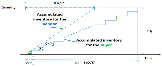
Figure 3.
Inventory pattern for the vendor.
That is:
inserting in the above equation:
simplifying by the sum of sequence formula:
Further simplification of the above equation:
Therefore, the vendor’s holding cost per unit time is:
As a certain amount of electrical energy is consumed during the holding time, the cost associated with the energy during the holding time is . Therefore, the vendor’s holding cost became:
The vendor’s expected annual cost with the recognition of electrical energy consumption cost is shown in Equation (1), and comprises the process quality improvement, setup cost reduction, setup cost, holding cost of the vendor, and defective cost:
3.2. Buyer’s Model
In this section, a buyer’s inventory model is developed based on Ben-Daya and Hariga [5] study. The two-echelon supply chain model with imperfect production and efficient energy consumption is considered. In this continuous review inventory model, the vendor produces quantities to save the buyer’s holding cost. The quantity produced in a production cycle is delivered in shipments to the buyer. The buyer places an order of quantity of non-defective items from the vendor as soon as the inventory level falls to reorder point , where , and is the expected demand during lead time; is the safety factor that fulfills the probability that the buyer’s lead-time demand exceeds the reorder point ; and is the safety stock (see Hadley and Whitin, [41] and Ben-Daya and Hariga [5]). The vendor replenishes the order quantity after the lead time. However, due to the imperfect production system in the batch, some items are defective; thus, the buyer cannot sell all the replenished items. Hence, the buyer inspects the replenished products to separate the defective products from the non-defective products. This paper considered a 100% inspection of the buyer with screening rate x to locate the imperfect items in the lot, as mentioned in assumption 4. It is also assumed that the screening process is error-free and non-destructive. These defective products are identified, separated out, and returned to the vendor in the next lot.
The defective items can be reduced to some level, but cannot be eliminated entirely. These defective items create unexpected shortages in the system. To avoid the losses due to defective items in this model, the vendor sends an additional amount of inventory to the buyer, unlike in the previous studies of Huang [22] and Dey and Giri [6]. In the literature, the demand from the buyer is met by reducing the replenishment interval to (see [3,18,22]). However, the replenishment interval is not reduced in this model; to avoid the shortages due to imperfect products, the buyer orders additional products from the vendor. Consider the situation in which the buyer orders a quantity . The order quantity is approximated to because has a negligible value. Consequently, the vendor gives products to the buyer. This additional amount will fulfill the buyer’s demand and simultaneously compensate for the losses due to the imperfect production process. The flow of material is shown in Figure 4. The buyer has two types of holding cost for defective and non-defective items in this model.
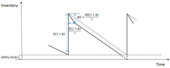
Figure 4.
Inventory of the buyer with inspection.
Buyer holding cost for defective products with energy consumption
The amount of defective products that the buyer receives is ; the defective rate is . The defective items’ quantity is approximated to due to the very small value of The number of defective items found is during the inspection time . It shows that the amount of average inventory of defective items per cycle is . The average inventory of the identified defective products per year is . The cost incurred on holding the average inventory of the defective product per year of the buyer is , and the electrical energy consumed during the holding period is . Therefore, the holding cost of the buyer is:
Buyer holding cost for non-defective products with energy consumption
The amount of non-defective products that the buyer receives is . The expected inventory of the non-defective product during the screening time is The holding cost incurred on the non-defective products per year is , and the cost of the energy consumed during holding these products is Thus, the buyer holding cost for non-defective products is:
Buyer screening cost with energy consumption
As products are screened with a per-unit screening cost of s and the cost of electrical energy consumed during screening being . Therefore, the annual screening cost is:
Buyer ordering cost with energy consumption
The buyer ordering cost per order is A, and the energy consumed during the ordering time is . The buyer cycle length is . Thus, the ordering cost of the buyer is:
Lead-time crashing cost with energy consumption cost
The lead time L consists of m mutually independent components, and these components include the order preparation time, order transit to the supplier, transit time from the supplier, setup time, and preparation time for availability. The component has a minimum duration of , normal duration of , and crashing cost per unit time of , and the cost of energy consumed during the crashing time is . Furthermore, for convenience, it is assumed that . It is clear that the lead-time reduction should start from the first component (the reason is the minimum crashing cost), and then the second component, and so on (Liao and Shyu [42], Ben-Daya and Hariga [5], and Kim et al. [23]). Let = and be the length of the lead-time components 1, 2, 3, …, z that crashed in their minimum duration; then, can be written as , where . The lead-time crashing cost per cycle with electrical energy consumption is , as shown in Equation (2) (see Ouyang and Wu [13]) for a given :
The buyer has to carry the additional costs incurred by the vendor on lead-time reduction in each stage of the replenishment cycle, and the lead-time crashing cost is also included in the buyer’s cost.
Transportation discounts with electrical energy consumption cost
The concept of a transportation discount is incorporated in this paper. The cost of transportation is not constant, and it depends directly on the demand function. In the literature, the transportation cost is considered as fixed, i.e., independent of ordering quantity or shipment in most of the cases. In this study, the transportation cost is dependent on the demand as (see Priyan and Uthayakumar [39], Shin et al. [34]):
where , is the transportation cost per unit. describes the range of ), i.e., should be in some specific range; else, cannot be defined. Since the energy is consumed during transportation, the cost associated with the energy consumption during the transportation is . Therefore, the transportation cost after considering the energy consumption cost will become as shown in Equation (3):
The expected annual cost of the buyer (), which consists of the ordering cost, lead-time crashing cost, holding cost for defective products, holding cost for non-defective products, screening cost, and the transportation discounts with electrical energy consumption during the process, is shown in Equation (4):
The service measure reflects that certain fractions of the demand, which is satisfied regularly from the available inventory, is expressed by .
The buyer service level in terms of the fill rate is described as shown in Equations (5) and (6):
which can be simplified as shown in Equation (7):
To obtain the least favourable distribution, the following lemma is used as shown in Equation (8) (Gallego and Moon [12]):
As or (see Hadley and Whitin, [41] and Ben-Daya and Hariga [5]), suppose that , and it became as shown in Equation (9):
After solving Equation (9), it will become as shown in Equation (10):
After inserting the value of y in Equation (10), it will become as shown in Equation (11):
Inserting the value of in Equation (4), the annual expected cost of the buyer with energy consumption cost is shown in Equation (12):
3.3. Supply Chain Cost
3.3.1. Centralized Analysis
The expected annual cost concerning the supply chain model with electrical energy consumption is sum of the vendor costs (as in Equation (1)) and the buyer’s cost (as in Equation (4)). Accordingly, the can be represented as shown in Equation (13):
In the above Equation (13), the cost components include: the investment made for quality improvement, the initial investments for the setup cost reduction, the setup cost with the energy consideration of the vendor, the ordering cost with the energy cost of the buyer, the holding cost of the defective items with the energy consideration of the buyer, the buyer non-defective item-holding cost, the screening cost with energy consideration, the holding cost of the vendor, the replacement cost with energy consideration, and the transportation discount cost with energy cost, respectively.
The necessary conditions to get the minimum cost of with energy consideration are as follows in Equations (14)–(17):
The optimal values for the decision variables are calculated by using the necessary conditions as follows in Equations (18)–(21):
where:
The optimal values of n are obtained by the expression shown in Equation (22):
Sufficient conditions are satisfied by taking the second derivative of the decision variable with respect to the expected annual cost.
From the sufficing conditions, the following values are obtained as shown in Equations (23)–(25):
To find the global minimum , the lemma is shown in Appendix A.
This Algorithm 1 is developed to determine the numerical solution of the proposed model, and the process flow of the algorithm is shown in Figure 5. Below is the detailed explanation of the algorithm to obtaining the optimal solution of the problem.
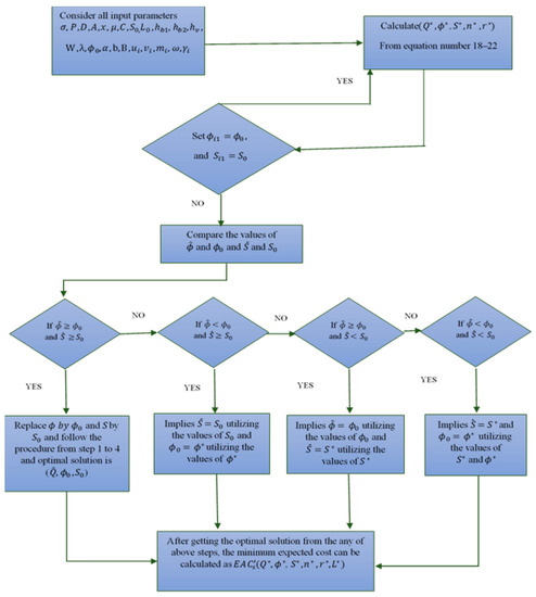
Figure 5.
Flowchart of the algorithm.
| Algorithm 1. Solution algorithm. | |
| Step 1 | Consider all input parameters, |
| Step 2 | For each and execute Steps 2.1 to 2.2. |
| Step 2.1 | Set and |
| Step 2.2 | Substitute the value of and in Equation (18) to evaluate |
| Step 2.3 | Use the value of to obtain , and from Equations (19) and (20). |
| Step 2.4 | Suppose , and repeat the above steps from 2.2 and 2.3 until no changes occur in the values of ; then, denote the solution by and . |
| Step 3 | In this step, and and and are compared. |
| Step 3.1 | If and , then the values obtained in Step 2 are the optimal solution for the given ; express this solution by ) and then proceed to Step 4. |
| Step 3.2 | If and , then set S = and use Step 2 to determine the () values from Equation (18) and Equation (20). If , then the optimal solution for given is ) = () and progress to Step 5. Otherwise, go to Step 3.3. |
| Step 3.3 | If and , then set and use Step 2 to calculate new () values from Equations (18) and (19). If , then the optimal solution for given is ) = (), and then proceed to Step 4. Otherwise, move to Step 3.4. |
| Step 3.4 | and ; then set and and utilize Step 2 for calculating from Equation (18). Then, denote these values as ) = () and move to Step 3. |
| Step 4 | If all , k = 1, 2, 3, …, K are greater than or less than , chose the nearest , and stop. Otherwise, calculate the of the two nearest point using Equation (20) and select the , with the least joint total cost. Express this solution by the vector . |
| Step 5 | Choose the minimum cost for each |
| Step 5.1 | = . |
| Step 5.2 | Let , and repeat Steps 2 to 5 until satisfying an inequality, . |
| Step 6 | Choose the minimum cost for each and calculate the reorder point |
3.3.2. Decentralized Analysis (Stackelberg Approach)
In the Stackelberg approach, the buyer and the vendor are considered as two different entities each trying to minimize their own total cost. Hence, one is considered as the leader to decide the optimal decision and impose on the follower.
The two possible cases in this situation are presented in the following part.
Case 1: Vendor as a leader and buyer as a follower
In the first case, the vendor is the leader and buyer is the follower. Therefore, the buyer decides his optimal decision first. The buyer determines his optimal order quantity, the lead time, and the reorder point. The aim of the vendor is the reduction of the setup cost, the number of shipments, and the percentage of defects after taking inputs from the buyer’s optimal decisions.
The expected annual cost of the buyer with energy cost consideration is given in Equation (26):
and the expected annual cost of the vendor with energy consideration is given by Equation (27):
The analytical approach is applied to optimize the expected annual cost of the buyer. The partial derivative of the buyer’s cost with respect to the order quantity is shown in Equation (28), and the partial derivative of lead time is shown in Equation (29):
The optimal values of the vendor are decided by considering the buyer’s optimal decisions as inputs shown in Equations (30) and (31):
Further, the second-order derivative of the buyer’s ordering cost is shown in Equation (32):
The second-order derivative of the vendor’s decision variables are shown in Equations (33) and (34):
To find the optimal value of the order quantity, the partial derivatives of are equated to zero; thus, the optimal is shown in Equation (35):
The vendor will take the inputs from the buyer’s optimal decision and compute his optimal decision, as shown in Equations (36) and (37):
Case 2: Buyer as a leader and vendor as a follower
In this case, the buyer is the leader and vendor is the follower. Therefore, the vendor optimizes his order quantity, the number of shipments, the reduction in setup cost, and the process quality improvement. The buyer will optimize the reorder point and the lead time based on the vendor optimal decision variables.
The expected annual cost of the vendor with energy consumption cost is shown in Equation (38):
and the expected annual cost of the buyer with energy consumption cost is presented in Equation (39):
The expected annual cost of the vendor is optimized using an analytical method. The partial derivative of vendor costs with respect to the order quantity, the reduction in setup cost, and the defective percentage are shown in Equations (40)–(42):
Further, the second-order derivatives with respect to decision variable are shown in Equations (43) and (44):
To obtain the optimal values of the lot size, the setup cost, and the process quality improvement, the partial derivatives of are equated to zero. The optimal values are shown in Equations (45)–(47):
4. Numerical Examples
The following two numerical examples are considered to demonstrate the practical applicability of the proposed supply chain management model with relation to the electrical energy consumption. The data for the lead-time components shown in Table 3 are taken from Ouyang and Wu [13], but in their model, the cost of electrical energy consumption is not considered. However, in this numerical example, the lead time is reduced by considering an additional crashing cost and electrical energy consumption cost, as the first component cost reduction is minimum, and the energy consumed during this component is also minimum. Moving toward the second and third components, the cost increase with the energy consumption is presented in Table 3. The transportation cost structure presented in Table 4 (from Shin et al. [34]) is used in both numerical examples. However, in their model, they did not consider the cost of energy consumption with the transportation cost. In the given examples, the cost of electricity consumption is recognized, and the cost structure is shown in Table 4. The discount is offered for a certain transportation quantity; however, as the quantity increases, the consumption of energy also increases. Therefore, the cost of energy consumption increases in the transportation cost structure.
Table 3.
Components of lead time.
Table 4.
Transportation cost structure.
Example 1.
The following parametric values (from Dey and Giri [6]) are used in the numerical analysis of the proposed model. , , , , , , , , , , , , , , , , , , .
The impact of the lead time on with all the decision variables is shown in Table 5, and it is quite clear that when the lead time is three weeks, then the expected annual costs of the supply chain is minimum in comparison of four, six, and eight weeks based on the numerical example. From Table 5, it is also clear that when the lead time is minimal—i.e., the cost of energy consumption was minimal—that is the reason that the total cost is minimal. If the lead time is increased, during the waiting time, the energy is still consumed. Simultaneously, the effect of the changes on the related decision is also shown.
Table 5.
Impact of lead time on and other decision variables.
In Table 6, the is calculated when the investment is made for the production quality improvement and without any additional initial capital investment. Based on the numerical study, it can be concluded that there was a large reduction in the total supply chain cost with investment in process quality improvement and setup cost reduction. The initial investment for setup cost reduction and quality improvement also affect the energy consumption of the supply chain, which is shown in Table 6, and lowers the overall supply chain costs.
Table 6.
Comparison of with and without investment in the reduction of the setup cost and quality enhancing.
Table 7 shows the comparative results for the improvement in the process quality and the reduction in the setup cost with no investment for quality improvement. Based on the numerical experiment, the investment made for quality improvement reduces the supply chain cost by improving the process quality. In Table 7, investments are not made for quality improvement, which means that the consumption of energy is relatively high, but the overall supply chain cost is still less than the cost without initial investments for quality improvement and setup cost reduction. The reason for total cost reduction is savings from the setup cost reduction through investment in advanced technology in the form of machines with less energy consumption.
Table 7.
Comparison of with and without investment in quality improvement.
In Table 8, the comparison of results are shown, when investments are made for process quality improvement and setup cost reduction, with a fixed setup cost. From the numerical study, it is clear that a huge amount of money can be saved by the incorporation initial investment for the setup cost. The investment in setup cost reduction is very effective in total cost reduction for this model, because it gives the opportunity for to vendor to use advanced technologies in production that consume energy effectively. Moreover, from Table 8, if initial investments are not made for quality improvement, the overall cost is increased. The reason behind that is the wastage due to poor quality and more energy consumption due to reproduction and by holding the defective items.
Table 8.
with investment in setup cost reduction and no investment for setup cost.
Table 5, Table 6, Table 7 and Table 8 present the results of the centralized supply chain. Table 9 shows the decentralized supply chain optimal values, and based on the numerical experiment, it is clear that the centralized system is better with low cost. Furthermore, in the decentralized supply chain context, when the buyer is the leader, the total cost of the supply chain is less compared to the case when the vendor is the leader by keeping same cost parameters.
Table 9.
Comparative results for the centralized and decentralized supply chain management policies.
The impact of the decision variables on the expected annual cost is shown graphically in the figures below. Based on the data from numerical Example 1, and from Figure 6, it is quite clear that the total cost of the supply chain is optimum when the buyer orders 176 items from the vendor; accordingly, any change in the order quantity by keeping the other decision variables the same, increases the expected annual cost of the supply chain. The setup cost relationship is shown in Figure 7, which shows that when the setup cost is $140, then the optimum supply chain costs are obtained, and any further variation increases the overall cost.
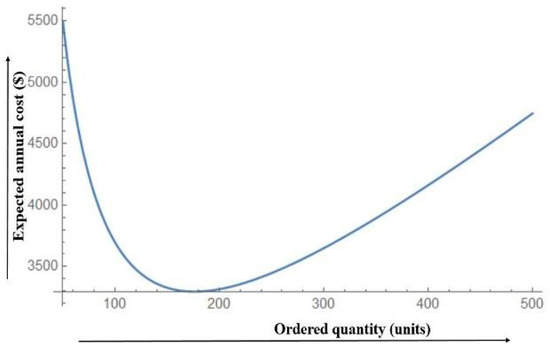
Figure 6.
Order quantity versus.
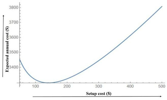
Figure 7.
Setup cost versus .
Figure 8 shows the relation between the out-of-control probability and the expected annual cost; the expected annual cost is optimum when the defective percentage is 0.0018, and changing the percentage of defective items increases the total supply chain cost. Similarly, from Figure 9, based on the data in numerical Example 1, the optimum number of shipments is 2, and any variation in the number of shipments—keeping the other parameters the same—will increase the expected annual cost of the supply chain.
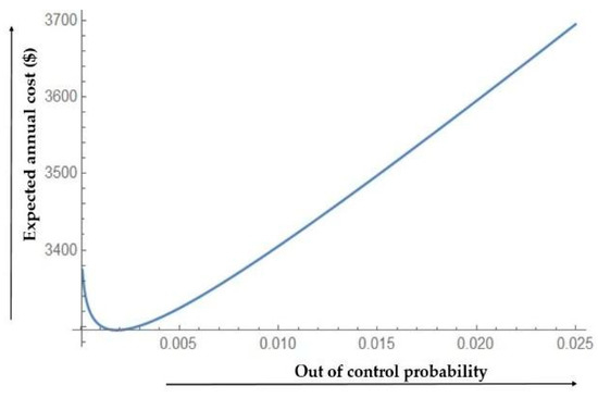
Figure 8.
Out-of-control probability versus .
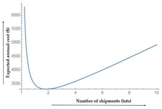
Figure 9.
Number of shipments versus .
Example 2.
The following parametric values (from Salameh and Jaber [3]) were used in the numerical analysis. , , , , , , , , , , , , , , , , , , , and .
Table 10 shows the impact of the lead time on the other decision variables and on the total cost. Based on the data shown in numerical Example 2, it is clear that the minimum cost is achieved when the lead time is four weeks. If the lead time increases from four weeks, it ultimately increases the total cost of the supply chain. In that case, more energy is consumed due to the increased lead time. Therefore, the lead crashing cost is used with energy consumption cost to reduce the lead time and energy consumption in this model.
Table 10.
Impact of lead time on and decision variables.
In Table 11, the comparison of the optimal costs of the proposed supply chain model and the optimal cost without investment in the process quality improvement and the setup cost reduction is provided. The reduction in the expected annual cost of the supply chain clearly describes the importance of initial capital investments for process quality improvement and setup cost reduction. The total cost of the supply chain reduces by the efforts made through initial capital investments. These investments are utilized for purchasing the technological upgraded machinery, which consumed less energy and improved production. Thus, these investments helped reduce the total supply chain costs.
Table 11.
Comparison of with reduction in setup cost and quality improvement, and fixed setup cost and quality.
The effect of investment in quality improvement on total cost is depicted in Table 12; further, it is quite clear after comparing it with the model in which no investment was made for quality, which increases the expected annual cost. From Table 12, it is quite clear that the initial capital invested for quality improvement is utilized in innovative ways to reduce the defective item percentage in the model. The total cost is decreased by quality improvement because of the production of less defective items, which consumed less energy.
Table 12.
Comparison of with and without investment in quality improvement.
In Table 13, the comparison is shown in which investments are made in the setup cost, with no initial capital investment. Consequently, the initial capital investment for the setup cost reduces the total supply chain costs with lower energy consumption in the supply chain model.
Table 13.
with investment in setup cost reduction and quality with no investments for both.
The effect on total cost with the decision variable is graphically shown in the following figures. Based on the data from numerical Example 2, Figure 10 shows that the optimal order quantity Q is 1802 units, and that further change in the order quantity—keeping the other parameters the same—increases the expected annual cost. Figure 11 depicts that the optimal setup cost is $129 for the model based on the data from numerical Example 2; any change in the setup cost without changing the other parameters increases the expected annual cost of the supply chain.
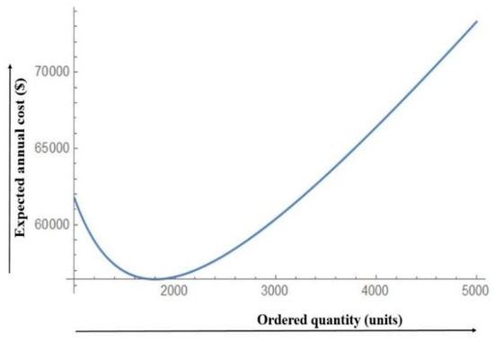
Figure 10.
Order quantity versus .
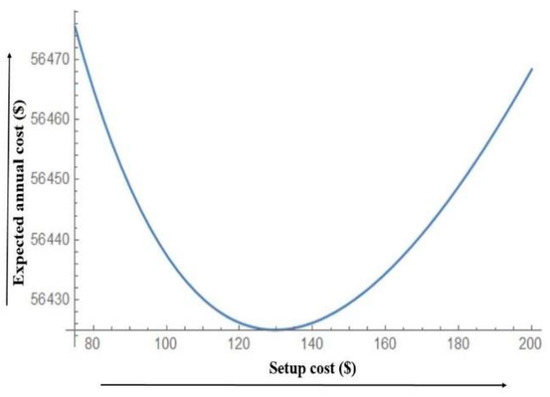
Figure 11.
Setup cost versus .
The effect of a change in the out-of-control probability is shown in Figure 12 for the annual expected cost. From Figure 13, based on the data from numerical Example 2, it is quite clear that the optimal number of shipments is two, and increasing or decreasing the number of shipments increases the annual expected cost.
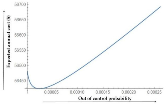
Figure 12.
Out-of-control probability versus .
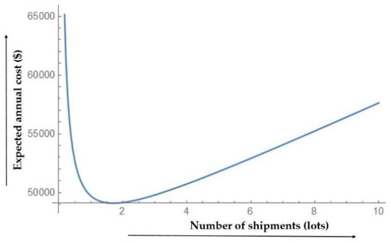
Figure 13.
Number of shipments versus .
5. Sensitivity Analysis
The sensitivity analysis is done for all the key parameters of the optimal values for Example 1, and is shown in Table 14. The values of the key parameters are varied from –50% to +50%, respectively, and the remaining parameters are unchanged. The effect of these parameters on the decision variables is calculated. The percentage variation in the optimal cost illustrates the following crucial features.
Table 14.
Sensitivity analysis for key parameters.
- If the investment in the quality is reduced by 50%, a small increase in the expected annual cost is observed, which means that the quality of the product is affected, and the extra energy is consumed through reproducing and keeping defective items. Similarly, if the investment in the quality is reduced by 25%, then a significant increase in the total cost is observed due to extra energy consumption on the defective items. The capital cost is more sensitive to the increase in investment than to its reduction.
- The negative change for the capital investment in setup cost reduces the total cost, but if the setup cost increases, the total cost also increases. The capital investment for the setup cost reduces the optimal order quantity.
- The fractional cost for the capital investment has an asymmetrical effect on the total cost, and it is considered as a sensitive parameter in this model. If the capital investments are reduced by 25%, the cost increases by 25%.
- The holding cost of the buyer for defective items is less sensitive than the total cost, because the amount of the defective products is less.
- The holding cost of the buyer’s non-defective items is the most sensitive parameter. If the holding decreases by 50%, the total cost reduces by 7%. Further, a 50% increase in the holding cost leads to an increase in the total cost by 16%. The inventory of the buyer’s non-defective items is more in quantity in this supply chain model; this is the reason behind the increase in total cost, and it consumes more energy.
- The variation in the holding cost of the vendor affects the total cost. If the holding cost decreases, the total cost reduces. Similarly, by increasing the holding cost, the total cost increases. A huge amount of energy is consumed while holding the products, and it also increases the holding cost, which ultimately increases the total cost of the supply chain model.
- The screening cost with energy consumption cost has a symmetrical effect on the total cost differently from the other parameters, which has an asymmetric impact on the entire cost of the supply chain, and it has no effect on the other decision variables. The screening cost includes the energy consumption cost during the screening and the variation observed for –50% and +50% is around 4% of the total cost of the supply chain.
- If the cost for the defective unit replacement with the energy consumption cost is decreased by 50%, then the total cost is reduced by a small percentage; however, if the decrement is 25%, then the total cost is increased by 10%. There is a small effect of positive percentage increase on the defective unit replacement cost.
6. Managerial Insights
Based on this study, the following recommendations are suggested for decision makers dealing with imperfect production in supply chain management:
- The major recommendation from this study for decision makers is the capital investment for process quality improvement. The investment is made for bringing in new technology, which uses optimum energy consumption; simultaneously, it reduces the probability that the system will move to an out-of-control state. It is proven from the numerical experiment that the investment reduces the total cost of the supply chain with minimum energy consumption.
- Another important insight for the present study from the decision maker’s point of view is the initial capital investment for setup cost reduction. This model suggests that decision makers ought to invest more initially to get the latest machinery and equipment, which can be used to reduce the whole supply chain cost with minimum energy consumption, as proven numerically.
- Due to the controllable lead time, if the buyer must make the decision related to lead-time reduction, by facing an additional crashing cost, he can reduce the lead time.
- In this model, the stockout costs are replaced with the service-level constraint, which helps managers overcome the difficult situations that occur due to the shortages, as well as the, enormous amount of energy consumed during the supply chain process. To avoid such situations, this model suggests the optimum level of inventory to be satisfied from the available stock to reduce energy consumption.
- In many cases, the objective of the managers is to minimize the cost by optimizing the decision variables. In this model, the energy costs are considered to elaborate the importance of the quantity of the consumed energy in the system, which is not considered in available supply chain models. If the cost incurred on the energy consumption is known to the managers, then the optimized level of energy consumption can be decided.
7. Conclusions
A two-echelon supply chain management model was developed in this study considering the effect of imperfect production, the inspection process, and energy consumption. The energy consumption related to the costs was not considered in previous research studies, and was proven to have numerous effects on the overall cost of the supply chain. As a result of introducing the energy consumption cost during the supply chain operation, a huge amount of money is saved. Furthermore, in this model, to reduce the shortages due to defective item production, the vendor sends an extra amount of quantity equal to the defective percentage to the buyer, and the collection of this amount takes place in the next batch. A lemma was constructed to show that the model attends a global optimal solution. This model encourages the managers to make an initial investment in order to improve the process quality and reduce the setup cost, which reduces the overall supply chain costs with enough energy consumption. Based on the analysis of the model, it was proven numerically that the centralized system is the most efficient compared to decentralized cases. However, in decentralized cases, the optimum cost is low when the buyer is a leader and the vendor is a follower. Based on numerical Example 1, the expected annual cost is optimum when the lead time is three weeks, and from numerical Example 2, the optimum expected annual cost is obtained when the lead time is four weeks. The effect of the initial investment made for quality improvement and setup cost reduction has a significant effect on the expected annual cost reduction and minimum energy consumption, as concluded from numerical examples. Furthermore, the graphical analysis is performed to show the impact of the variation in the lot size, the number of shipments, the setup cost, and the process quality by considering energy-related costs. The sensitivity analysis was performed to validate the proposed model. The proposed model in this paper can be extended in several aspects by including the green supply chain management with variable demand, multi-item production, a multi-buyer supply chain, and a region-based distribution network.
Author Contributions
Conceptualization, I.K. and B.S.; methodology, investigation, formal analysis, writing—original draft preparation, I.K.; conceptualization, resources, validation, writing—review and editing, visualization, supervision, B.S.; data curation, software, I.K. and J.J.; data curation and software, H.L.
Funding
There is no funding for the research paper.
Acknowledgments
The authors are thankful to three anonymous reviewers for their valuable comments to revise the older version of the paper.
Conflicts of Interest
The authors declare no conflict of interest.
Appendix A
Lemma 1.
If the Hessian matrix foris positive definite at the optimal valuesthencontains the global minimum at the optimum solution.
Proof.
To show that the Hessian matrix for is always positive definite, all minors must be positive definite, and the corresponding principal minors at the optimal values need to be:
It is proved that when all the principal minors are positive definite, contains the optimal solution Hence, the contains the global minimum at the optimal decision variable under the effect of optimum energy consumption. □
References
- Sarkar, M.; Sarkar, B. Optimization of safety stock under controllable production rate and energy consumption in an automated smart production management. Energies 2019, 12, 2059. [Google Scholar] [CrossRef]
- Sarkar, B.; Saren, S.; Sinha, D.; Hur, S. Effect of unequal lot sizes, variable setup cost, and carbon emission cost in a supply chain model. Math Probl. Eng. 2015, 2015, 469486. [Google Scholar] [CrossRef]
- Salameh, M.; Jaber, M. Economic production quantity model for items with imperfect quality. Int. J. Prod. Econ. 2000, 64, 59–64. [Google Scholar] [CrossRef]
- Ouyang, L.Y.; Chen, C.K.; Chang, H.C. Quality improvement, setup cost and lead-time reductions in lot size reorder point models with an imperfect production process. Comput. Oper. Res. 2002, 29, 1701–1717. [Google Scholar] [CrossRef]
- Ben-Daya, M.; Hariga, M. Integrated single vendor single buyer model with stochastic demand and variable lead time. Int. J. Prod. Econ. 2004, 92, 75–80. [Google Scholar] [CrossRef]
- Dey, O.; Giri, B. Optimal vendor investment for reducing defect rate in a vendor–buyer integrated system with imperfect production process. Int. J. Prod. Econ. 2014, 155, 222–228. [Google Scholar] [CrossRef]
- Khan, M.; Jaber, M.; Guiffrida, A.; Zolfaghari, S. A review of the extensions of a modified EOQ model for imperfect quality items. Int. J. Prod. Econ. 2011, 132, 1–12. [Google Scholar] [CrossRef]
- Chung, K.J. The economic production quantity with rework process in supply chain management. Comput. Math. Appl. 2011, 62, 2547–2550. [Google Scholar] [CrossRef]
- Tayyab, M.; Sarkar, B. Optimal batch quantity in a cleaner multi-stage lean production system with random defective rate. J. Clean. Prod. 2016, 139, 922–934. [Google Scholar] [CrossRef]
- Cárdenas-Barrón, L.E.; Taleizadeh, A.A.; TreviñO-Garza, G. An improved solution to replenishment lot size problem with discontinuous issuing policy and rework, and the multi-delivery policy into economic production lot size problem with partial rework. Expert Syst. Appl. 2012, 39, 13540–13546. [Google Scholar] [CrossRef]
- Scarf, H. A min-max solution of an inventory problem. In Studies in the Mathematical Theory of Inventory and Production; Stanford University Press: Redwood City, CA, USA, 1958. [Google Scholar]
- Gallego, G.; Moon, I. The distribution free newsboy problem: Review and extensions. J. Oper. Res. Soc. 1993, 44, 825–834. [Google Scholar] [CrossRef]
- Ouyang, L.Y.; Wu, K.S. Mixture inventory model involving variable lead time with a service level constraint. Comput. Oper. Res. 1997, 24, 875–882. [Google Scholar] [CrossRef]
- Moon, I.; Choi, S. The distribution free continuous review inventory system with a service level constraint. Comput. Ind. Eng. 1994, 27, 209–212. [Google Scholar] [CrossRef]
- Tajbakhsh, M.M. On the distribution free continuous-review inventory model with a service level constraint. Comput. Ind. Eng. 2010, 59, 1022–1024. [Google Scholar] [CrossRef]
- Ma, W.M.; Qiu, B.B. Distribution-free continuous review inventory model with controllable lead time and setup cost in the presence of a service level constraint. Math. Probl. Eng. 2012, 2012, 867847. [Google Scholar] [CrossRef]
- Harris, F.W. How many parts to make at once. In Factory, The Magazine of Management; University of Michigan: Arbor, MI, USA, 1913. [Google Scholar]
- Cárdenas-Barrón, L.E. Observation on:” Economic production quantity model for items with imperfect quality” [Int. J. Production Economics 64 (2000) 59-64]. Int. J. Prod. Econ. 2000, 67, 201. [Google Scholar]
- Ciavotta, M.; Meloni, C.; Pranzo, M. Minimising general setup costs in a two-stage production system. Int. J. Prod. Res. 2013, 51, 2268–2280. [Google Scholar] [CrossRef]
- Dellino, G.; Kleijnen, J.P.; Meloni, C. Robust optimization in simulation: Taguchi and response surface methodology. Int. J. Prod. Econ. 2010, 125, 52–59. [Google Scholar] [CrossRef]
- Goyal, S.K.; Cárdenas-Barrón, L.E. Note on: Economic production quantity model for items with imperfect quality–A practical approach. Int. J. Prod. Econ. 2002, 77, 85–87. [Google Scholar] [CrossRef]
- Huang, C.K. An optimal policy for a single-vendor single-buyer integrated production–inventory problem with process unreliability consideration. Int. J. Prod. Econ. 2004, 91, 91–98. [Google Scholar] [CrossRef]
- Kim, M.S.; Kim, J.S.; Sarkar, B.; Sarkar, M.; Iqbal, M.W. An improved way to calculate imperfect items during long-run production in an integrated inventory model with backorders. J. Manuf. Syst. 2018, 47, 153–167. [Google Scholar] [CrossRef]
- Sarkar, B. Supply chain coordination with variable backorder, inspections, and discount policy for fixed lifetime products. Math Probl. Eng. 2016, 2016, 6318737. [Google Scholar] [CrossRef]
- Tang, L.; Che, P.; Liu, J. A stochastic production planning problem with nonlinear cost. Comput. Oper. Res. 2012, 39, 1977–1987. [Google Scholar] [CrossRef]
- Gahm, C.; Denz, F.; Dirr, M.; Tuma, A. Energy-efficient scheduling in manufacturing companies: A review and research framework. Ejor 2016, 248, 744–757. [Google Scholar] [CrossRef]
- Keller, F.; Reinhart, G. Energy Supply Orientation in Production Planning Systems. Procedia Cirp 2016, 40, 244–249. [Google Scholar] [CrossRef]
- Du, Y.; Hu, G.; Xiang, S.; Zhang, K.; Liu, H.; Guo, F. Estimation of the diesel particulate filter soot load based on an equivalent circuit model. Energies 2018, 11, 472. [Google Scholar] [CrossRef]
- Todde, G.; Murgia, L.; Caria, M.; Pazzona, A. A comprehensive energy analysis and related carbon footprint of dairy farms, Part 2: Investigation and modeling of indirect energy requirements. Energies 2018, 11, 463. [Google Scholar] [CrossRef]
- Tomić, T.; Schneider, D.R. The role of energy from waste in circular economy and closing the loop concept–Energy analysis approach. Renew. Sustain. Energy Rev. 2018, 98, 268–287. [Google Scholar] [CrossRef]
- Haraldsson, J.; Johansson, M.T. Review of measures for improved energy efficiency in production-related processes in the aluminium industry–From electrolysis to recycling. Renew. Sustain. Energy Rev. 2018, 93, 525–548. [Google Scholar] [CrossRef]
- Ouyang, L.Y.; Chang, H.C. Impact of investing in quality improvement on (Q, r, L) model involving the imperfect production process. Prod. Plan. Cont. 2000, 11, 598–607. [Google Scholar] [CrossRef]
- Porteus, E.L. Optimal lot sizing, process quality improvement and setup cost reduction. Oper. Res. 1986, 34, 137–144. [Google Scholar] [CrossRef]
- Shin, D.; Guchhait, R.; Sarkar, B.; Mittal, M. Controllable lead time, service level constraint, and transportation discounts in a continuous review inventory model. Rairo-Oper. Res. 2016, 50, 921–934. [Google Scholar] [CrossRef]
- Braglia, M.; Castellano, D.; Song, D. Distribution-free approach for stochastic Joint-Replenishment Problem with backorders-lost sales mixtures, and controllable major ordering cost and lead times. Comput. Oper. Res. 2017, 79, 161–173. [Google Scholar] [CrossRef]
- Tsao, Y.C.; Lu, J.C. A supply chain network design considering transportation cost discounts. Trans. Res. Part E Log. Rev. 2012, 48, 401–414. [Google Scholar] [CrossRef]
- Ouyang, L.Y.; Chen, L.Y.; Yang, C.T. Impacts of collaborative investment and inspection policies on the integrated inventory model with defective items. Int. J. Prod. Res. 2013, 51, 5789–5802. [Google Scholar] [CrossRef]
- Jha, J.; Shanker, K. An integrated inventory problem with transportation in a divergent supply chain under service level constraint. J. Manuf. Syst. 2014, 33, 462–475. [Google Scholar] [CrossRef]
- Priyan, S.; Uthayakumar, R. Trade credit financing in the vendor–buyer inventory system with ordering cost reduction, transportation cost and backorder price discount when the received quantity is uncertain. J. Manuf. Syst. 2014, 33, 654–674. [Google Scholar] [CrossRef]
- Gutgutia, A.; Jha, J. A closed-form solution for the distribution free continuous review integrated inventory model. Oper. Res. 2018, 18, 159–186. [Google Scholar] [CrossRef]
- Hadley, G.; Whitin, T.M. Analysis of Inventory Systems: G. Hadley, TM Whitin; Prentice-Hall: Upper Saddle River, NJ, USA, 1963. [Google Scholar]
- Liao, C.J.; Shyu, C.H. An analytical determination of lead time with normal demand. Int. J. Oper. Prod. Manag. 1991, 11, 72–78. [Google Scholar] [CrossRef]


© 2019 by the authors. Licensee MDPI, Basel, Switzerland. This article is an open access article distributed under the terms and conditions of the Creative Commons Attribution (CC BY) license (http://creativecommons.org/licenses/by/4.0/).