Economic Analysis of an Integrated Production–Inventory System under Stochastic Production Capacity and Energy Consumption


Abstract
1. Introduction
2. Problem Statement, Notation, and Assumptions
2.1. Problem Statement
| Notation | |
| Decision variables | |
| Q | Production lot size (units) |
| p | Production rate, where (units/unit time) |
| The manufacturing reliability parameter, where | |
| Model parameters | |
| T | Replenishment cycle time (year) |
| Setup cost ($/setup) | |
| J | Restoration cost ($/setup) |
| x | Demand rate (units/unit time) |
| Unit production cost, function of reliability and productivity ($) | |
| M | Raw material cost ($/unit) |
| r | Raw material increment cost due to manufacturing unreliability ($/unit) |
| L | Unit manufacturing yield loss cost due to manufacturing unreliability ($/unit/unit time) |
| Tool/die cost ($/unit) | |
| Scale parameter | |
| A | Production-technology development cost, cost to increase production rate by one unit ($) |
| Productivity scale parameter | |
| Productivity shape parameter | |
| Technology development cost ($) | |
| Reliability constant, non-negative | |
| Reliability scale parameter | |
| Inventory holding cost ($/unit/unit time) | |
| Repair rate (repairs/unit time) | |
| Corrective repair cost ($/unit time) | |
| Opportunity cost due to lost sales ($/lost unit) | |
| Random variable denoting time to manufacturing system failure (non-negative) | |
| Random variable denoting time to repair upon system failure (non-negative) | |
| Probability density function, cumulative density function of | |
| Probability density function, cumulative density function of | |
| Expected total cost per cycle with manufacturing system failure ($) | |
| Expected total cost per cycle without manufacturing system failure ($) | |
| Expected cycle length with manufacturing system failure (time) | |
| Expected cycle length without manufacturing system failure (time) | |
| Expected total cost per unit time with manufacturing system failure ($) | |
| Expected total cost per unit time without manufacturing system failure ($) | |
| Expected total cost per unit time of manufacturing system ($) |
2.2. Assumptions
- -
- The demand rate of the products is known and constant, whereas the controllable production rate of manufacturing system is greater than demand rate , and a decision variable.
- -
- The unit production cost is not constant but a function of controllable processing rate and manufacturing unreliability.
- -
- The reliability of the manufacturing system is derived through a stochastic process.
- -
- The reliability of manufacturing system is expressed as a design variable, where it is represented as , and reliability can be increased through investment in production technology and manufacturing resources.
- -
- The failure rate and repair rate are random variables and follow continuous probability distributions.
- -
- The manufacturing reliability and production rate are considered as energy control variables, independent and additive.
- -
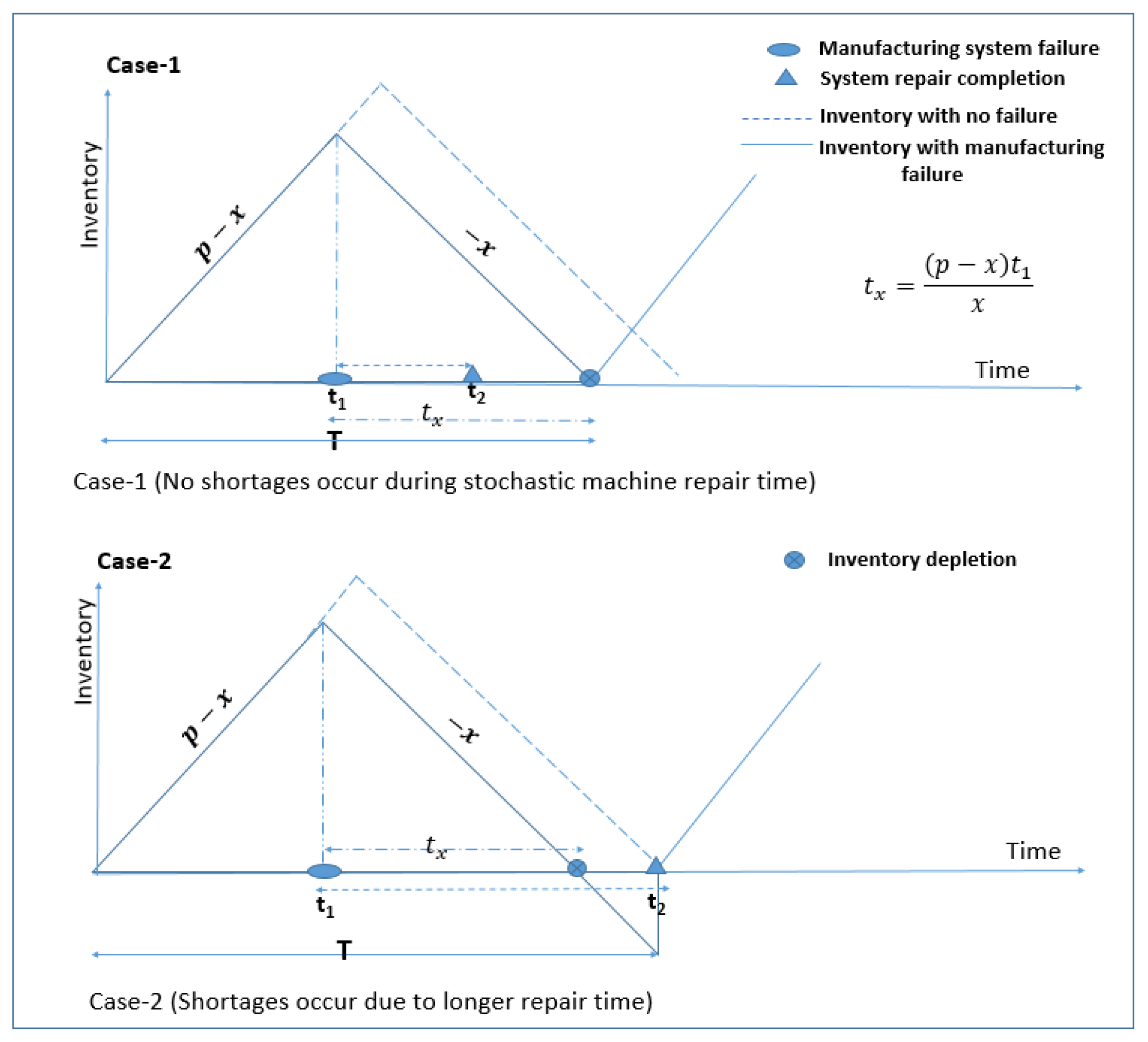
- Shortages are considered for longer repair duration.
3. Mathematical Model
3.1. Model 1: Random Production Capacity Model with Manufacturing System Failure
| Energy parameters | |
| Unit cost of electrical energy ($/kWh) | |
| Expected energy cost for production ($) | |
| Fixed component of required energy for manufacturing system (kWh/time) | |
| Variable component of required energy for production process (kWh/unit) | |
| Expected energy cost for machine repair ($) | |
| Energy required for repair time (kWh/unit time) | |
| Energy required for each production setup (kWh/setup) | |
| Energy required for each minor restoration (kWh/setup) | |
| Energy required for inventory holding (kWh/unit/unit time) |
- The cost component is the cost of raw material, which increases linearly with increasing failure rate of manufacturing system.
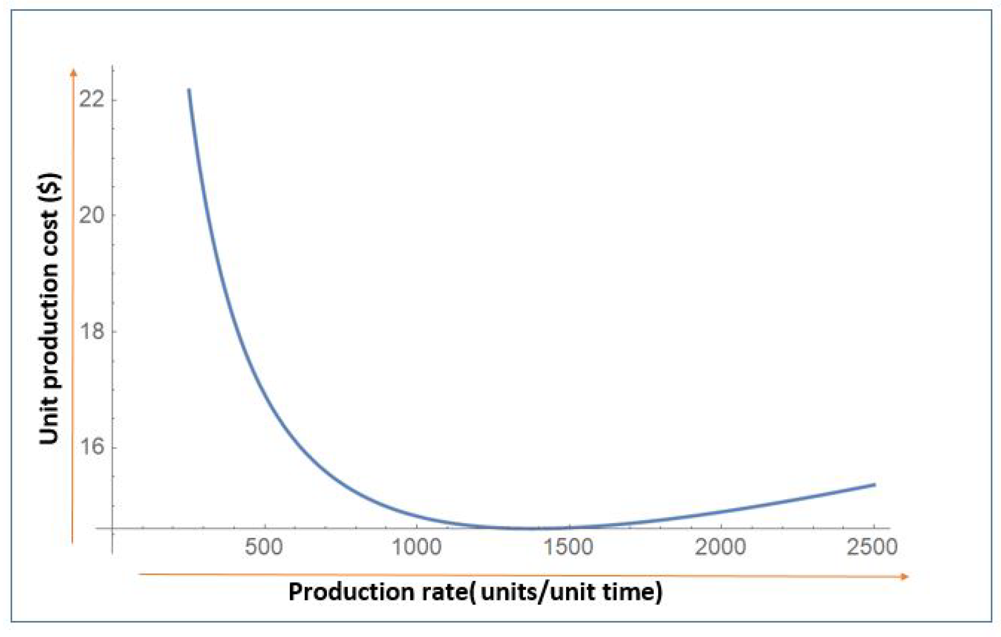
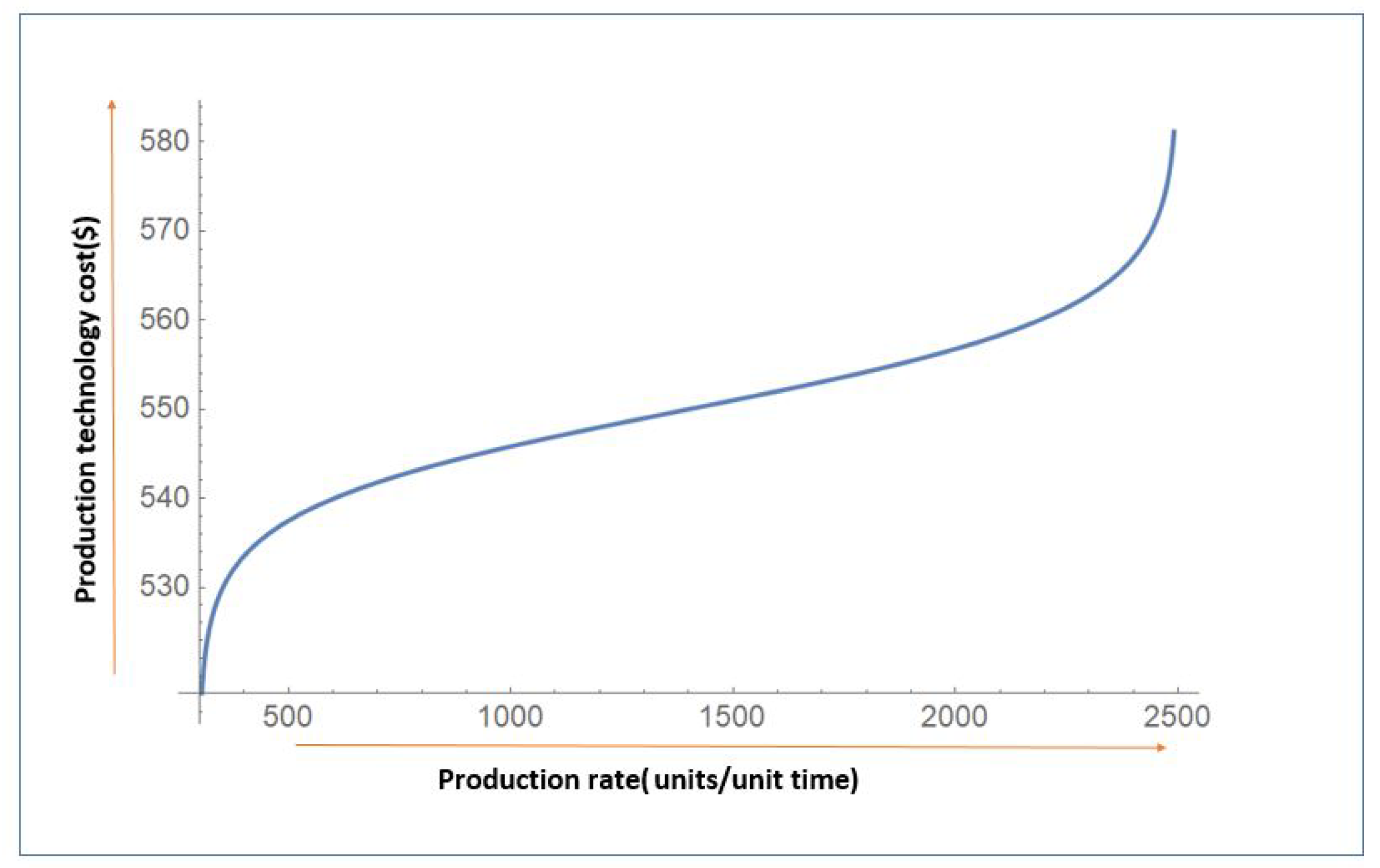
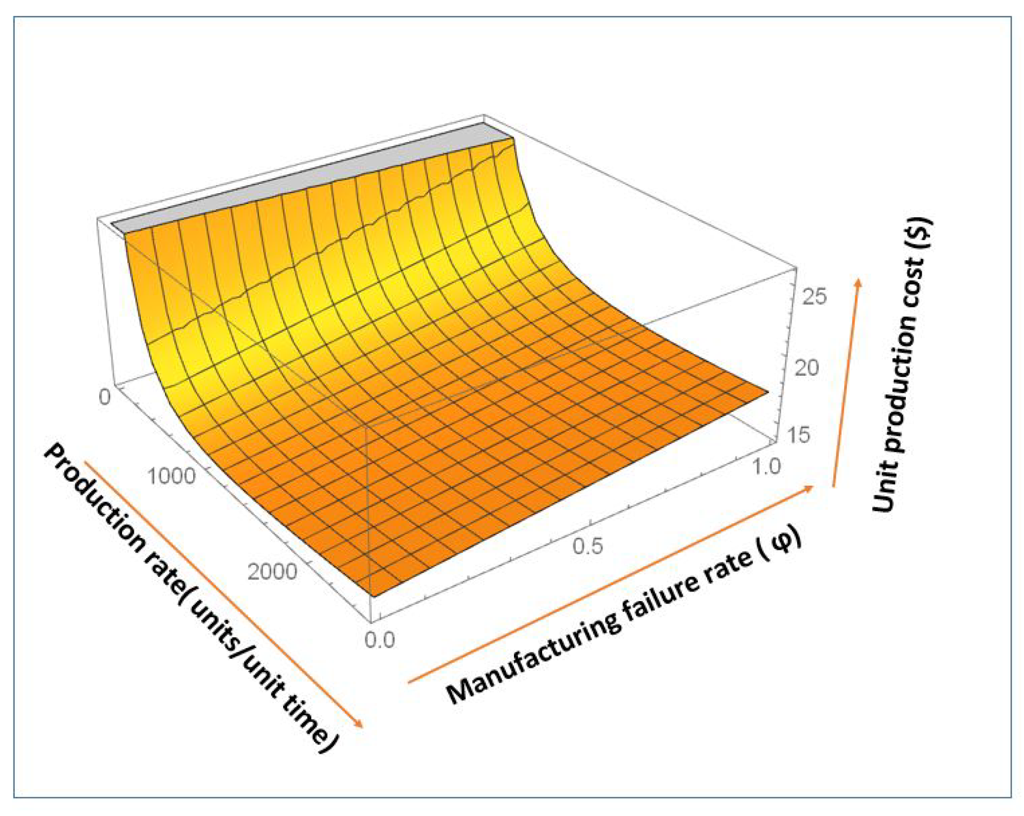
- The component represents the manufacturing costs, i.e., capital and labor costs, and, as the production rate increases, manufacturing cost is evenly distributed across a vast number of produced units. Consequently, the per unit manufacturing cost reduces with higher production rates (see Figure 2).
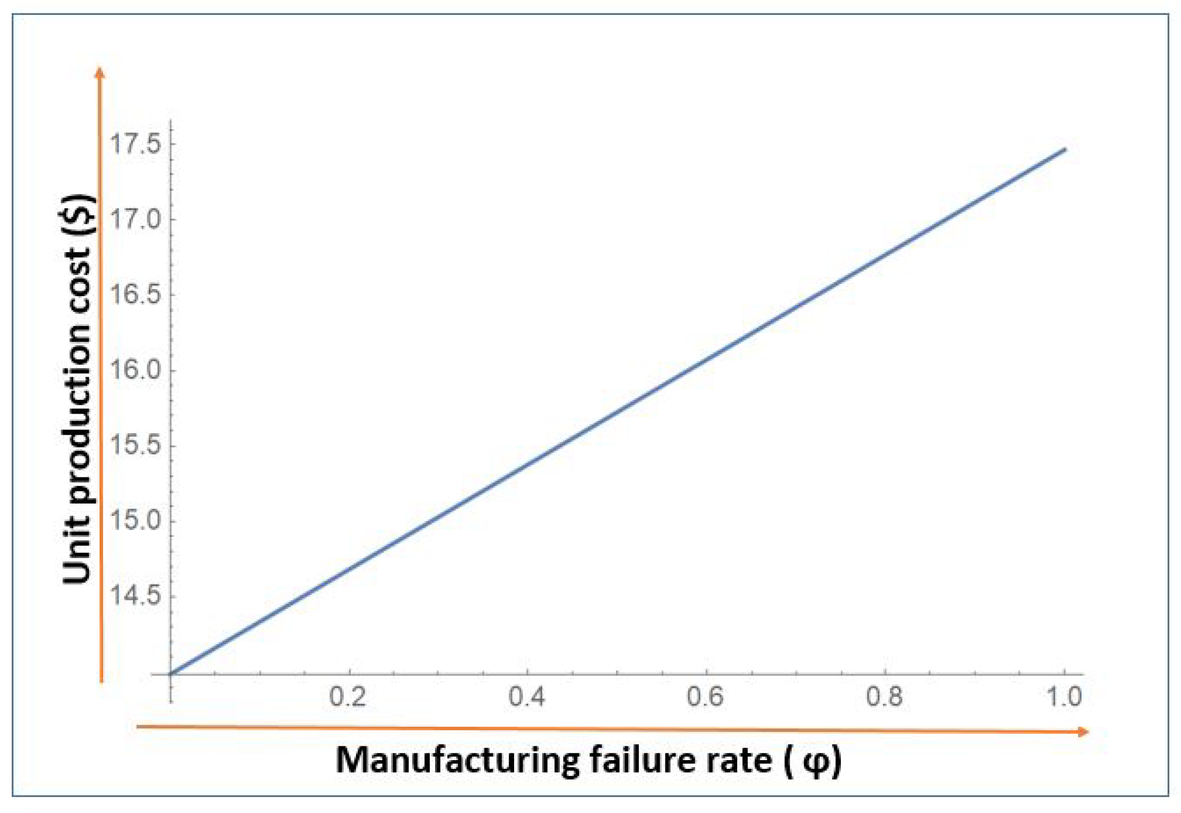
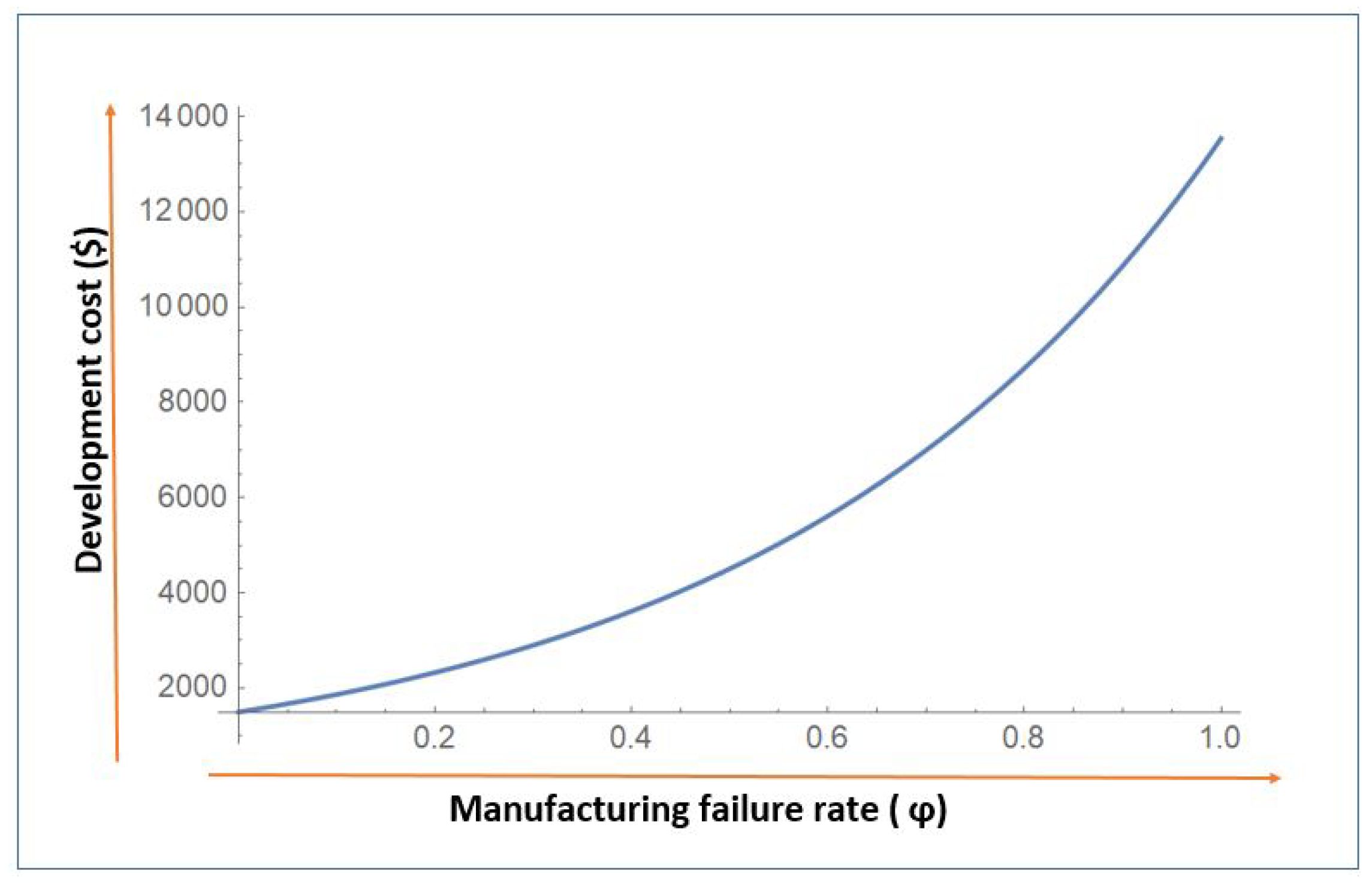
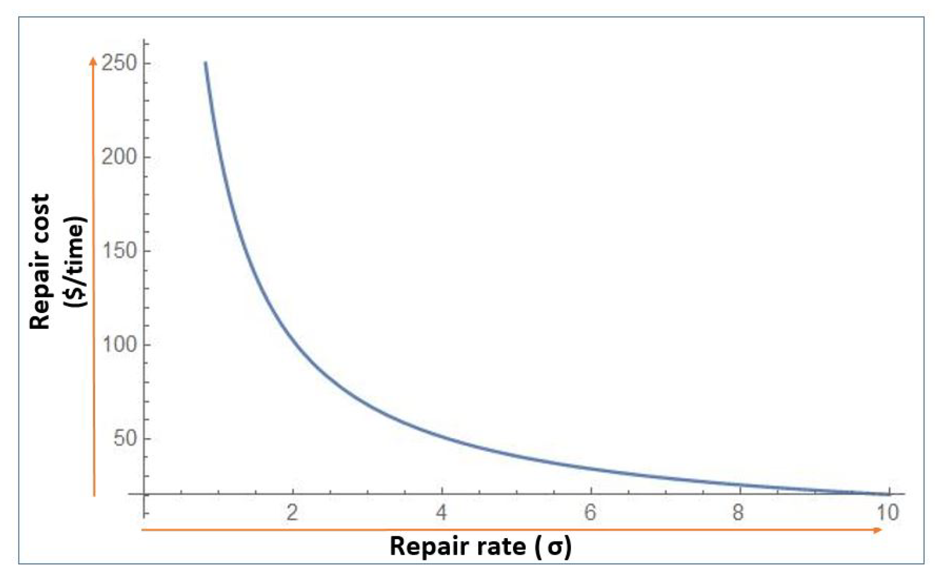
- The next cost component is , which represents the manufacturing yield loss. As the failure rate of manufacturing system increases, the downtime increases and overall costs of system increases linearly (see Figure 3). However, with higher production rates, the unit yield loss cost decreases as the higher production rate reduces the production up-time and more items are produced in fewer working hours.
- The last cost component is referred to as tool/die cost, and it is directly proportional to production rate.
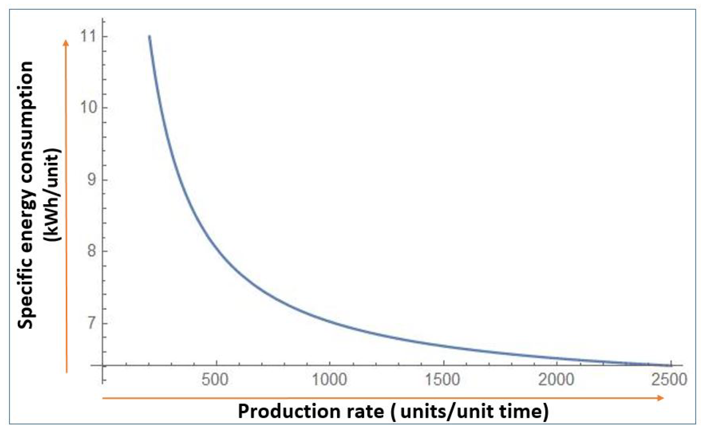
- The energy cost for production is given as a function of electrical energy consumption (kWh) based on controllable production rate. Therefore, expected energy cost for a production run is derived as a function of unit electricity cost ($/kWh), specific energy required per item produced (kWh/unit), production up-time (hours), and production rate p (units/unit time).Moreover, as the unit manufacturing cost is equally distributed over a wide range of produced products, per unit production cost becomes,
3.2. Model 2: Random Production Capacity Model without System Failure
3.3. Integrated Stochastic Capacity-Reliability Model
3.4. Solution Methodology
4. Numerical Experiment
4.1. Example
4.2. Sensitivity Analysis
- Higher setup costs increase the total cost of manufacturing system but decrease the production rate of system. The proposed model also suggests increase in production quantity Q for higher setup costs to avoid multiple setup costs. On the other hand, the restoration cost J shows an increasing pattern for production quantity, production rate and expected total cost of the system. As the restoration cost depends on two parameters, setup cost and manufacturing reliability of system, the increasing value of restoration cost suggest higher production lot to avoid multiple setup requirement. In addition, it suggests higher production rates to shorten the production up-time to avoid added costs of longer production runs and possible system failure.
- For the decreasing shortage cost , the model shows insensitivity to production lot size. However, in the case of an increase in shortage cost in the model, we see an increase in manufacturing reliability and decrease in the production lot size.
- Inventory holding cost h shows no impact on manufacturing reliability in this model. However, an increase in holding cost suggests an increase in production rate along with reduction of production quantity to reduce inventory accumulation. Higher inventory holding costs lead to higher system costs. The energy cost for inventory holding shows the same pattern as inventory holding cost. With decreasing energy requirements for inventory carrying, the model suggests an increase in production lot size and production rate. Manufacturing reliability is insensitive to energy requirements for inventory holding.
- The technology development cost has direct impact on the manufacturing reliability and productivity of system. The manufacturing reliability is defined as a system-design variable and it represents the number of failures a system faces during operational hours. As the increase in technology investment shows a reduction in reliability parameter, it also reduces the production rate of system to adjust the total optimal cost of system. The production quantity increases with higher development costs, as it shows a more reliable manufacturing system.
- With the increase in corrective maintenance cost , the model suggests an increase in production rate to adjust the optimal total cost of the system. Higher corrective maintenance cost leads to smaller production quantities, and the expected total cost of system also increases due to higher maintenance costs. The increasing value of suggest an increase in production quantity; as represents the mean time to repair, as the mean time to repair decreases, the idle time for manufacturing system decreases. In addition, the model shows increase in production rate and the expected total cost of system; as the productivity of manufacturing system increases, the machine is in operational state for longer periods of time.
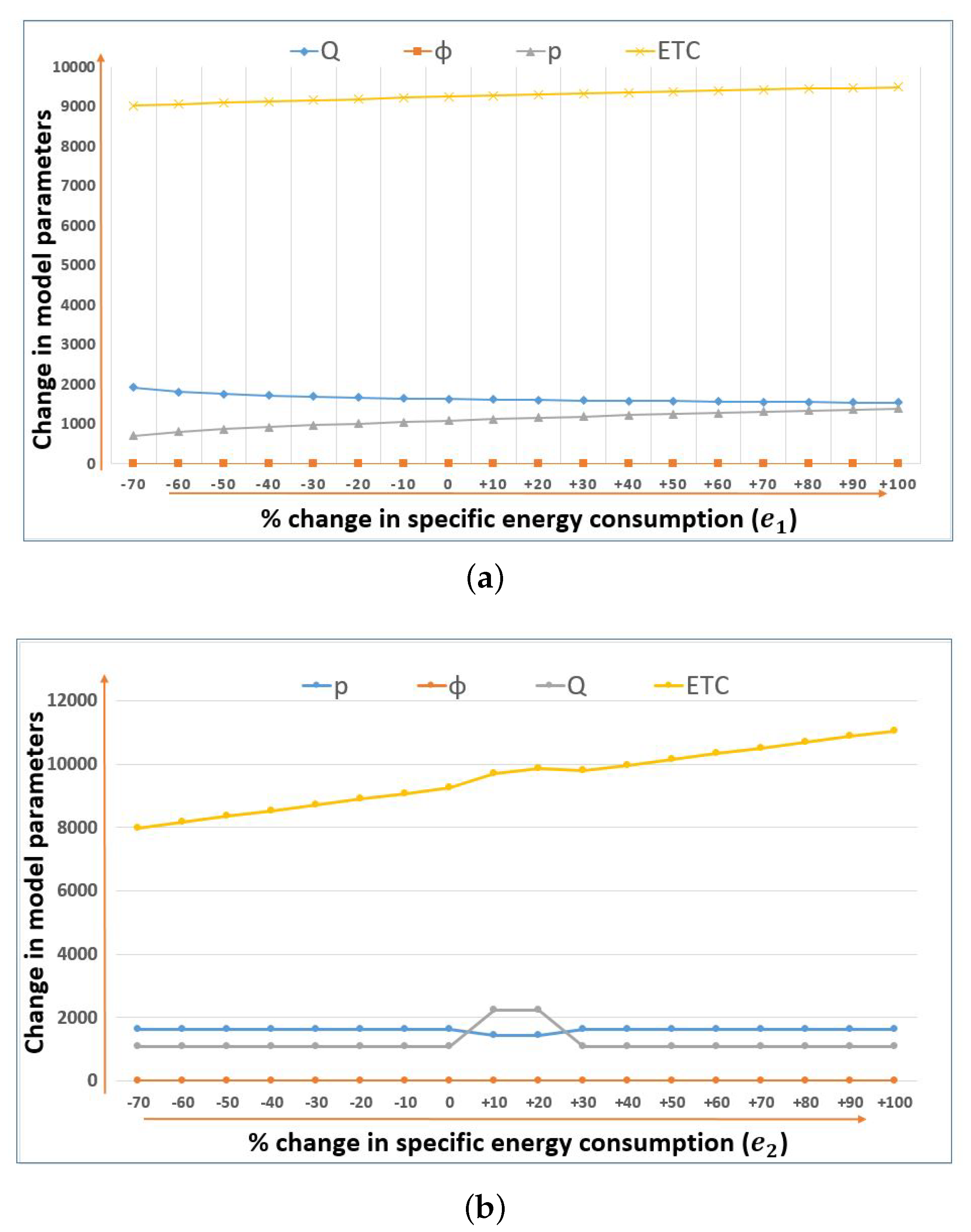
- As the required energy cost for system repair increases, the model shows a reduction in production quantity but increase in production rate. The reduction in production lot size explains that, as total energy required for maintenance increases, the specific energy consumption per unit for repair increases. Therefore, the model suggest an increase in production rate to optimize the production policy under energy consumption. The total expected cost also increases with an increase in required electrical energy for repair activities.
- Unit production cost comprises labor and specific energy consumption costs required to produce a production quantity; as the unit manufacturing cost decreases, we see an increase in production lot size of the model. In addition, with decrease in unit manufacturing cost, the expected total cost and production rate decreases. For both labor and production energy cost , as the production rate decreases, the optimal reliability parameter also decreases, which is due to lower stress on the manufacturing system. Moreover, as production lot increases, reliability decreases to adjust technology development cost.
- The raw material cost M and raw material yield loss cost r both are highly sensitive to any increasing values of model parameters. The increase in material yield loss cost increases the production quantity and production rate simultaneously to adjust the total expected cost. In addition, it shows a reduction in the optimal reliability parameter of the model that is quite obvious; as for the manufacturing system, where raw material yield loss adds significant cost to manufacturing, higher reliability parameter is optimal for manufacturing system.
- The increase in tool/die cost shows a reduction in optimal production rate. As the production rate of manufacturing system increases, the added load/stress on manufacturing system increases the maintenance requirement of such machinery, and, to adjust the higher cost of production-technology development, the model suggests reduction in reliability value and optimal production rate.
- The manufacturing yield loss L due to manufacturing system failures also increases the expected total cost of the system. Moreover, the increase in manufacturing yield loss cost suggests a decrease in production quantity and justifies increasing the production rate to improve the productivity of the system. The increase in yield loss value suggests reducing the manufacturing reliability parameter to minimize the negative effect of manufacturing system failures.
- As the unit cost A to increase production rate by one unit decreases, the model shows an increase in production rate. With the increase in the production rate, the reliability parameter also increases. As the higher stress value increases failure frequency of manufacturing system, reliability parameter increases accordingly to adjust the technology development cost to keep total cost at an optimal limit. The productivity constants show quite unique trends; as the value of productivity scale parameter increases, the production rate decreases continuously with an increasing trend in production quantity and expected total cost of system. However, it is insensitive towards manufacturing reliability parameter. The productivity shape parameter is insensitive towards expected total cost and reliability parameter of the system, however an increase in shape parameter increases the production quantity and decreases the production rate monotonically.
4.2.1. Comparative Study
4.2.2. Managerial Insights
- The study provides a better understanding of production–maintenance policy for stochastic production capacities under random failure rates, random repair rates and energy consumption requirements.
- By employing precise cost data of related cost factors associated with unreliable manufacturing systems, production and maintenance managers can set an optimum level of manufacturing reliability that minimizes the overall maintenance and energy consumption costs.
- Random breakdowns of manufacturing system represent an inevitable phenomenon, which is considered in many maintenance planning models for energy consumption, but the effect of random repair rate is usually ignored. This study also gives insights into the simultaneous improvement of reliability and manufacturing productivity when managers faces the challenge of uncertain production capacities due to longer repair times.
- The increase in tool/die cost shows a reduction in optimal production rate. As the production rate of manufacturing system increases, the added load and stress increases the maintenance requirement of such machinery, and to adjust the higher cost of production-technology development, the model suggests reductions in reliability value and processing speeds.
- For controllable production rates, the added expenditure of maintenance and technology development investment are also considered; therefore, managers can also look into possible technology development needed to improve productivity of manufacturing systems.
- This paper presents the relevant relationships between variable energy consumption rates and constituents related to stochastic production capacities and maintenance management plans. Improved production and maintenance planning will allow managers to increase production rates and reduce energy consumption per unit of production quantity. Furthermore, through additional production and technology development policies, machine breakdowns can be reduced.
5. Conclusions
- The study suggested that it is not practical to consider constant production rates in an unreliable manufacturing system; as the system faces random failure rate and random repair rate, the productivity of system is highly affected due to manufacturing unreliability. In such a scenario, controllable production rates help in increasing the production capacity of a manufacturing system.
- As the productivity of a manufacturing system depends on its reliability and operational condition, the unit production cost of a manufacturing system is considered as a function of controllable production rate, which varies within design limits, manufacturing reliability, labor costs and variable energy costs.
- The manufacturing system productivity and reliability can be further enhanced through investment in advance technology, better and improved resources and skilled labor. Therefore, a production-technology development cost is introduced as a function of manufacturing reliability. For improved efficiency of manufacturing process, a productivity investment is also introduced in manufacturing costs to get optimal level of variable processing speeds for an unreliable manufacturing system.
- The cost of electrical energy consumption for simultaneous production, inventory and maintenance planning is not considered in the existing literature, therefore this study introduces the energy cost components for operational and idle states of production setups, restoration, production, inventory holding and repair cost.
- A limitation of the study is considering deterministic demand, where random demand of products is a more realistic phenomena. In addition, only electrical energy consumption is considered in this study, whereas production firms usually use more than one type of energy sources in production. The model can be further extended with the case of imperfect production process, inspection policies and economic factors such as inflation and time value of money. Moreover, integrated production–maintenance policies under uncertain production environments are worthy of investigation, as discussed in [53]. The study can be further extended to the concept [54] of imperfect production process for an unreliable manufacturing system, as production of defectives is inevitable.
Author Contributions
Funding
Conflicts of Interest
Abbreviations
| EMQ | Economic manufacturing quantity |
| O2O | Online to Offline |
| AR | Abort/Resume |
| KT | Kuhn–Tucker method |
| SEC | Specific energy consumption |
| EEPP | Energy efficient production planning |
References
- Sarkar, B.; Guchhait, R.; Sarkar, M.; Pareek, S.; Kim, N. Impact of safety factors and setup time reduction in a two-echelon supply chain management. Robot. Comput.-Integr. Manuf. 2019, 55, 250–258. [Google Scholar] [CrossRef]
- Ciavotta, M.; Meloni, C.; Pranzo, M. Minimising general setup costs in a two-stage production system. Int. J. Prod. Res. 2013, 51, 2268–2280. [Google Scholar] [CrossRef]
- Kumar, V.; Sarkar, B.; Sharma, A.N.; Mittal, M. New product launching with pricing, free replacement, rework, and warranty policies via genetic algorithmic approach. Int. J. Comput. Int. Syst. 2019, 12, 519–529. [Google Scholar] [CrossRef]
- Sarkar, B.; Guchhait, R.; Sarkar, M.; Cárdenas-Barrón, L.E. How does an industry manage the optimum cash flow within a smart production system with the carbon footprint and carbon emission under logistics framework? Int. J. Prod. Econ. 2019, 213, 243–257. [Google Scholar] [CrossRef]
- Shibin, K.; Gunasekaran, A.; Papadopoulos, T.; Childe, S.J.; Dubey, R.; Singh, T. Energy sustainability in operations: An optimization study. Int. J. Adv. Manuf. Technol. 2016, 86, 2873–2884. [Google Scholar] [CrossRef][Green Version]
- Bazan, E.; Jaber, M.Y.; Zanoni, S. Supply chain models with greenhouse gases emissions, energy usage and different coordination decisions. Appl. Math. Model. 2015, 39, 5131–5151. [Google Scholar] [CrossRef]
- Giret, A.; Trentesaux, D.; Prabhu, V. Sustainability in manufacturing operations scheduling: A state of the art review. J. Manuf. Syst. 2015, 37, 126–140. [Google Scholar] [CrossRef]
- Liu, Y.; Dong, H.; Lohse, N.; Petrovic, S.; Gindy, N. An investigation into minimising total energy consumption and total weighted tardiness in job shops. J. Clean. Prod. 2014, 65, 87–96. [Google Scholar] [CrossRef]
- Biel, K.; Glock, C.H. Systematic literature review of decision support models for energy-efficient production planning. Comput. Ind. Eng. 2016, 101, 243–259. [Google Scholar] [CrossRef]
- Liu, Y.; Dong, H.; Lohse, N.; Petrovic, S. A multi-objective genetic algorithm for optimisation of energy consumption and shop floor production performance. Int. J. Prod. Econ. 2016, 179, 259–272. [Google Scholar] [CrossRef]
- Rapine, C.; Penz, B.; Gicquel, C.; Akbalik, A. Capacity acquisition for the single-item lot sizing problem under energy constraints. Omega 2018, 81, 112–122. [Google Scholar] [CrossRef]
- Mousavi, S.; Thiede, S.; Li, W.; Kara, S.; Herrmann, C. An integrated approach for improving energy efficiency of manufacturing process chains. Int. J. Sustain. Eng. 2016, 9, 11–24. [Google Scholar] [CrossRef]
- González-Romera, E.; Ruiz-Cortés, M.; Milanés-Montero, M.I.; Barrero-González, F.; Romero-Cadaval, E.; Lopes, R.A.; Martins, J. Advantages of minimizing energy exchange instead of energy cost in prosumer microgrids. Energies 2019, 12, 719. [Google Scholar] [CrossRef]
- Mori, M.; Fujishima, M.; Inamasu, Y.; Oda, Y. A study on energy efficiency improvement for machine tools. CIRP Ann. 2011, 60, 145–148. [Google Scholar] [CrossRef]
- Shrouf, F.; Ordieres-Meré, J.; García-Sánchez, A.; Ortega-Mier, M. Optimizing the production scheduling of a single machine to minimize total energy consumption costs. J. Clean. Prod. 2014, 67, 197–207. [Google Scholar] [CrossRef]
- Tang, D.; Dai, M.; Salido, M.A.; Giret, A. Energy-efficient dynamic scheduling for a flexible flow shop using an improved particle swarm optimization. Comput. Ind. 2016, 81, 82–95. [Google Scholar] [CrossRef]
- Dai, M.; Tang, D.; Giret, A.; Salido, M.A.; Li, W.D. Energy-efficient scheduling for a flexible flow shop using an improved genetic-simulated annealing algorithm. Robot. Comput.-Integr. Manuf. 2013, 29, 418–429. [Google Scholar] [CrossRef]
- Li, X.; Xing, K.; Wu, Y.; Wang, X.; Luo, J. Total energy consumption optimization via genetic algorithm in flexible manufacturing systems. Comput. Ind. Eng. 2017, 104, 188–200. [Google Scholar] [CrossRef]
- Calicioglu, O.; Flammini, A.; Bracco, S.; Bellù, L.; Sims, R. The Future Challenges of Food and Agriculture: An integrated analysis of trends and solutions. Sustainability 2019, 11, 222. [Google Scholar] [CrossRef]
- Pramangioulis, D.; Atsonios, K.; Nikolopoulos, N.; Rakopoulos, D.; Grammelis, P.; Kakaras, E. A Methodology for Determination and Definition of Key Performance Indicators for Smart Grids Development in Island Energy Systems. Energies 2019, 12, 242. [Google Scholar] [CrossRef]
- Brahman, F.; Honarmand, M.; Jadid, S. Optimal electrical and thermal energy management of a residential energy hub, integrating demand response and energy storage system. Energy Build. 2015, 90, 65–75. [Google Scholar] [CrossRef]
- Shojafar, M.; Cordeschi, N.; Baccarelli, E. Energy-efficient adaptive resource management for real-time vehicular cloud services. IEEE Tran. Cloud Comput. 2016, 7, 196–209. [Google Scholar] [CrossRef]
- Sarkar, B.; Tayyab, M.; Choi, S.B. Product Channeling in an O2O supply chain management as power transmission in electric power distribution systems. Mathematics 2019, 7, 4. [Google Scholar] [CrossRef]
- Bazan, E.; Jaber, M.Y.; Zanoni, S. Carbon emissions and energy effects on a two-level manufacturer-retailer closed-loop supply chain model with remanufacturing subject to different coordination mechanisms. Int. J. Prod. Econ. 2017, 183, 394–408. [Google Scholar] [CrossRef]
- Bazan, E.; Jaber, M.Y.; El Saadany, A.M. Carbon emissions and energy effects on manufacturing-remanufacturing inventory models. Comput. Ind. Eng. 2015, 88, 307–316. [Google Scholar] [CrossRef]
- Sarkar, M.; Sarkar, B.; Iqbal, M. Effect of energy and failure rate in a multi-item smart production system. Energies 2018, 11, 2958. [Google Scholar] [CrossRef]
- Devoldere, T.; Dewulf, W.; Deprez, W.; Willems, B.; Duflou, J.R. Improvement potential for energy consumption in discrete part production machines. In Advances in Life Cycle Engineering for Sustainable Manufacturing Businesses; Springer: London, UK, 2007; pp. 311–316. [Google Scholar]
- Sarkar, B.; Sana, S.S.; Chaudhuri, K. Optimal reliability, production lotsize and safety stock: An economic manufacturing quantity model. Int. J. Manag. Sci. Eng. Manag. 2010, 5, 192–202. [Google Scholar] [CrossRef]
- Sarkar, B.; Sana, S.S.; Chaudhuri, K. Optimal reliability, production lot size and safety stock in an imperfect production system. Int. J. Math. Oper. Res. 2010, 2, 467–490. [Google Scholar] [CrossRef]
- Sarkar, B. An inventory model with reliability in an imperfect production process. App. Math. Comput. 2012, 218, 4881–4891. [Google Scholar] [CrossRef]
- Bhuniya, S.; Sarkar, B.; Pareek, S. Multi-product production system with the reduced failure rate and the optimum energy consumption under variable demand. Mathematics 2019, 7, 465. [Google Scholar] [CrossRef]
- Yao, X.; Zhou, J.; Zhang, J.; Boër, C.R. From intelligent manufacturing to smart manufacturing for Industry 4.0 driven by next generation artificial intelligence and further On. In Proceedings of the 2017 5th International Conference on Enterprise Systems (ES), Beijing, China, 22–24 September 2017; IEEE: Piscataway, NJ, USA, 2017; pp. 311–318. [Google Scholar]
- Sarkar, B.; Mandal, P.; Sarkar, S. An EMQ model with price and time dependent demand under the effect of reliability and inflation. App. Math. Comput. 2014, 231, 414–421. [Google Scholar] [CrossRef]
- Glock, C.H. Batch sizing with controllable production rates. Int. J. Prod. Res. 2010, 48, 5925–5942. [Google Scholar] [CrossRef]
- Shepherd, R.W. Theory of Cost and Production Functions; Princeton University Press: Princeton, NJ, USA, 2015. [Google Scholar]
- Rishel, R. Control of systems with jump Markov disturbances. IEEE Trans. Autom. Control 1975, 20, 241–244. [Google Scholar] [CrossRef]
- Olsder, G.; Suri, R. Time-optimal control of parts-routing in a manufacturing system with failure-prone machines. In Proceedings of the 1980 19th IEEE Conference on Decision and Control including the Symposium on Adaptive Processes, Albuquerque, NM, USA, 10–12 December 1980; IEEE: Piscataway, NJ, USA, 1980; pp. 722–727. [Google Scholar]
- Glock, C.H. Batch sizing with controllable production rates in a multi-stage production system. Int. J. Prod. Res. 2011, 49, 6017–6039. [Google Scholar] [CrossRef]
- Khouja, M.; Mehrez, A. Economic production lot size model with variable production rate and imperfect quality. J. Oper. Res. Soc. 1994, 45, 1405–1417. [Google Scholar] [CrossRef]
- Sarkar, M.; Hur, S.; Sarkar, B. Effects of variable production rate and time-dependent holding cost for complementary products in supply chain model. Math. Probl. Eng. 2017, 2017, 2825103. [Google Scholar] [CrossRef]
- Alfares, H.K.; Ghaithan, A.M. EOQ and EPQ Production-Inventory Models with Variable Holding Cost: State-of-the-Art Review. Arab. J. Sci. Eng. 2019, 44, 1737–1755. [Google Scholar] [CrossRef]
- Dey, B.K.; Sarkar, B.; Pareek, S. A two-echelon supply chain management with setup time and cost reduction, quality improvement and variable production rate. Mathematics 2019, 7, 328. [Google Scholar] [CrossRef]
- Khalifehzadeh, S.; Fakhrzad, M. A Modified Firefly Algorithm for optimizing a multi stage supply chain network with stochastic demand and fuzzy production capacity. Comput. Ind. Eng. 2019, 133, 42–56. [Google Scholar] [CrossRef]
- Marchi, B.; Zanoni, S.; Jaber, M.Y. Economic production quantity model with learning in production, quality, reliability and energy efficiency. Comput. Ind. Eng. 2019, 129, 502–511. [Google Scholar] [CrossRef]
- Marchi, B.; Zanoni, S.; Zavanella, L.; Jaber, M. Supply chain models with greenhouse gases emissions, energy usage, imperfect process under different coordination decisions. Int. J. Prod. Econ. 2019, 211, 145–153. [Google Scholar] [CrossRef]
- Adane, T.; Nicolescu, M. Towards a Generic Framework for the Performance Evaluation of Manufacturing Strategy: An Innovative Approach. J. Manuf. Mater. Process. 2018, 2, 23. [Google Scholar] [CrossRef]
- Demichela, M.; Baldissone, G.; Darabnia, B. Using field data for energy efficiency based on maintenance and operational optimisation. A step towards PHM in process plants. Processes 2018, 6, 25. [Google Scholar] [CrossRef]
- Rackow, T.; Kohl, J.; Canzaniello, A.; Schuderer, P.; Franke, J. Energy Flexible Production: Saving Electricity Expenditures by Adjusting the Production Plan. Procedia CIRP 2015, 26, 235–240. [Google Scholar] [CrossRef]
- Lee, S.; Prabhu, V.V. Energy-aware feedback control for production scheduling and capacity control. Int. J. Prod. Res. 2015, 53, 7158–7170. [Google Scholar] [CrossRef]
- Gutowski, T.; Dahmus, J.; Thiriez, A. Electrical energy requirements for manufacturing processes. In Proceedings of the 13th CIRP International Conference on Life Cycle Engineering, Leuven, Belgium, 31 May–2 June 2006; Volume 31, pp. 623–638. [Google Scholar]
- Prevention, I.P. Control Reference Document on Best Available Techniques for Large Combustion Plants; European Commission: Brussels, Belgium, 2006. [Google Scholar]
- Ross, S.M. Introduction to Probability Models; Academic Press: Cambridge, MA, USA, 2014. [Google Scholar]
- Dellino, G.; Kleijnen, J.P.; Meloni, C. Robust optimization in simulation: Taguchi and response surface methodology. Int. J. Prod. Econ. 2010, 125, 52–59. [Google Scholar] [CrossRef]
- Sarkar, B.; Majumder, A.; Sarkar, M.; Kim, N.; Ullah, M. Effects of variable production rate on quality of products in a single-vendor multi-buyer supply chain management. Int. J. Adv. Manuf. Technol. 2018, 99, 567–581. [Google Scholar] [CrossRef]


| Author(s) | Manufacturing Reliability | Maintenance Policy | Production Capacity | Development Cost | Energy |
|---|---|---|---|---|---|
| Marchi et al. [44] | variable | NA | variable | NA | considered |
| Marchi et al. [45] | variable | NA | variable | NA | considered |
| Bhuniya et al. [31] | variable | NA | variable | considered | |
| Sarkar et al. [26] | variable | NA | variable | considered | |
| Adane and Nicolescu [46] | NA | considered | constant | NA | NA |
| Demichela et al. [47] | NA | considered | NA | NA | considered |
| Li et al. [18] | NA | NA | flexible | NA | NA |
| Rackow et al. [48] | NA | NA | energy flexible | NA | considered |
| Shibin et al. [5] | NA | NA | flexible | NA | considered |
| Lee and Prabhu [49] | NA | considered | energy-aware | NA | considered |
| This study | stochastic | considered | controllable | considered |
| units/unit time) | per unit) | |
| per unit | kWh/unit/unit time) | |
| kWh) | setup) | |
| kWh/setup) | lost unit) | |
| unit/unit time) | ||
| kWh/unit time) | repairs/unit time) | |
| time) | units/unit time) | |
| units/unit time) | ||
| kWh/setup) | kWh/unit time) | kWh/unit) |
| Parameter | % Change | Q | p | % Change in | |
|---|---|---|---|---|---|
| −20 | 1611.36 | 0.24 | 1100.05 | −0.55 | |
| −10 | 1615.32 | 0.24 | 1099.61 | −0.46 | |
| +10 | 1654.56 | 0.24 | 1095.44 | ||
| +20 | 1673.92 | 0.24 | 1093.45 | ||
| J | −20 | 1628.46 | 0.23 | 1094.99 | −0.21 |
| −10 | 1631.75 | 0.23 | 1096.24 | −0.11 | |
| +10 | 1638.27 | 0.24 | 1098.75 | ||
| +20 | 1442.67 | 0.27 | 2253.6 | ||
| −20 | 1635.00 | 0.23 | 1097.20 | ||
| −10 | 1635.01 | 0.23 | 1097.36 | ||
| +10 | 1435.99 | 0.27 | 2262.39 | ||
| +20 | 1436.01 | 0.27 | 2262.40 | ||
| h | −20 | 1736.89 | 0.24 | 1134.34 | −2.32 |
| −10 | 1683.17 | 0.24 | 1115.96 | −1.14 | |
| +10 | 1587.60 | 0.24 | 1077.01 | ||
| +20 | 1552.56 | 0.24 | 1060.60 | ||
| −20 | 1635.01 | 0.23 | 1097.30 | ||
| −10 | 1635.02 | 0.23 | 1097.42 | ||
| +10 | 1435.98 | 0.27 | 2262.38 | ||
| +20 | 1435.99 | 0.27 | 2262.39 | ||
| −20 | 1700.41 | 0.24 | 1122.09 | −1.53 | |
| −10 | 1666.54 | 0.24 | 1109.82 | −0.76 | |
| +10 | 1605.64 | 0.24 | 1085.11 | ||
| +20 | 1578.21 | 0.24 | 1072.63 | ||
| −20 | 1633.61 | 0.24 | 1095.13 | −0.01 | |
| −10 | 1634.41 | 0.24 | 1096.58 | −0.01 | |
| +10 | 1635.51 | 0.24 | 1098.08 | ||
| +20 | 1635.90 | 0.24 | 1099.45 | ||
| −20 | 1635.50 | 0.24 | 1096.00 | −0.02 | |
| −10 | 1635.29 | 0.24 | 1096.66 | −0.01 | |
| +10 | 1634.76 | 0.24 | 1098.33 | ||
| +20 | 1634.50 | 0.24 | 1098.33 | ||
| −20 | 1635.23 | 0.23 | 1096.83 | −0.01 | |
| −10 | 1635.13 | 0.24 | 1097.16 | −0.00 | |
| +10 | 1634.92 | 0.24 | 1097.83 | ||
| +20 | 1634.82 | 0.24 | 1098.16 | ||
| −20 | 1550.14 | 0.26 | 1129.66 | −1.55 | |
| −10 | 1593.41 | 0.26 | 1113.23 | −0.76 | |
| +10 | 1675.26 | 0.26 | 1082.32 | ||
| +20 | 1710.49 | 0.26 | 1069.04 | ||
| −20 | 1578.13 | 0.26 | 1131.53 | −0.80 | |
| −10 | 1623.86 | 0.24 | 1104.14 | −0.16 | |
| +10 | 1670.69 | 0.23 | 1076.42 | ||
| +20 | 1689.53 | 0.22 | 1065.35 | ||
| −20 | 1698.76 | 0.21 | 1059.96 | ||
| −10 | 1668.95 | 0.23 | 1077.44 | ||
| +10 | 17,278 | 0.05 | 300.06 | −7.55 | |
| +20 | 22,244 | 0.05 | 300.17 | −7.76 |
| Parameter | % Change | Q | p | % Change in | |
|---|---|---|---|---|---|
| −20 | 1700.58 | 0.23 | 962.96 | −1.32 | |
| −25 | 1663.05 | 0.23 | 1034.12 | −0.64 | |
| +10 | 1436.44 | 0.27 | 2257.64 | ||
| +20 | 1594.67 | 0.24 | 1209.48 | ||
| −20 | 1672.19 | 0.23 | 1018.60 | −0.62 | |
| −10 | 1653.42 | 0.23 | 1058.36 | −0.31 | |
| +10 | 1623.49 | 0.24 | 1131.16 | ||
| +20 | 1608.94 | 0.24 | 1166.59 | ||
| −20 | 1637.45 | 0.23 | 1096.31 | −3.89 | |
| −10 | 1637.42 | 0.23 | 1096.02 | −1.94 | |
| +10 | 1439.66 | 0.24 | 2240.77 | ||
| +20 | 1439.76 | 0.27 | 2238.81 | ||
| r | −20 | 1629.01 | 0.24 | 1105.86 | −0.39 |
| −10 | 1631.99 | 0.24 | 1101.65 | −019 | |
| +10 | 1638.11 | 0.24 | 1093.39 | ||
| +20 | 1439.43 | 0.26 | 2246.64 | ||
| M | −20 | 1635.11 | 0.24 | 1098.46 | −8.03 |
| −10 | 1635.07 | 0.24 | 1097.98 | −4.02 | |
| +10 | 1634.98 | 0.24 | 1097.01 | ||
| +20 | 1436.76 | 0.27 | 2249.79 | ||
| −20 | 1583.03 | 0.25 | 1248.08 | −1.41 | |
| −10 | 1608.94 | 0.24 | 1166.81 | −0.68 | |
| +10 | 1637.65 | 0.24 | 1091.10 | ||
| +20 | 1688.38 | 0.23 | 984.278 | ||
| L | −20 | 1640.96 | 0.24 | 1079.23 | −0.24 |
| −10 | 1638.25 | 0.24 | 1087.43 | −0.13 | |
| +10 | 1631.98 | 0.23 | 1107.38 | ||
| +20 | 1629.09 | 0.23 | 1117.08 | ||
| A | −20 | 1627.73 | 0.24 | 1079.23 | −0.24 |
| −10 | 1632.59 | 0.24 | 1087.43 | −0.13 | |
| +10 | 1638.06 | 0.23 | 1107.38 | ||
| +20 | 1641.09 | 0.23 | 1117.08 | ||
| −20 | 1629.25 | 0.24 | 1098.87 | −0.12 | |
| −10 | 1632.59 | 0.24 | 1098.07 | −0.05 | |
| +10 | 1638.06 | 0.24 | 1096.77 | ||
| +20 | 1641.09 | 0.24 | 1096.05 | ||
| −20 | 1634.95 | 0.24 | 1097.71 | ||
| −10 | 1634.99 | 0.24 | 1097.60 | ||
| +10 | 1635.06 | 0.24 | 1097.39 | ||
| +20 | 1635.01 | 0.24 | 1097.28 |
© 2019 by the authors. Licensee MDPI, Basel, Switzerland. This article is an open access article distributed under the terms and conditions of the Creative Commons Attribution (CC BY) license (http://creativecommons.org/licenses/by/4.0/).
Share and Cite
Asghar, I.; Sarkar, B.; Kim, S.-j. Economic Analysis of an Integrated Production–Inventory System under Stochastic Production Capacity and Energy Consumption. Energies 2019, 12, 3179. https://doi.org/10.3390/en12163179
Asghar I, Sarkar B, Kim S-j. Economic Analysis of an Integrated Production–Inventory System under Stochastic Production Capacity and Energy Consumption. Energies. 2019; 12(16):3179. https://doi.org/10.3390/en12163179
Chicago/Turabian StyleAsghar, Iqra, Biswajit Sarkar, and Sung-jun Kim. 2019. "Economic Analysis of an Integrated Production–Inventory System under Stochastic Production Capacity and Energy Consumption" Energies 12, no. 16: 3179. https://doi.org/10.3390/en12163179
APA StyleAsghar, I., Sarkar, B., & Kim, S.-j. (2019). Economic Analysis of an Integrated Production–Inventory System under Stochastic Production Capacity and Energy Consumption. Energies, 12(16), 3179. https://doi.org/10.3390/en12163179