Abstract
Water flooding is an economic method commonly used in secondary recovery, but a large quantity of crude oil is still trapped in reservoirs after water flooding. A deep understanding of the distribution of residual oil is essential for the subsequent development of water flooding. In this study, a pore-scale model is developed to study the formation process and distribution characteristics of residual oil. The Navier–Stokes equation coupled with a phase field method is employed to describe the flooding process and track the interface of fluids. The results show a significant difference in residual oil distribution at different wetting conditions. The difference is also reflected in the oil recovery and water cut curves. Much more oil is displaced in water-wet porous media than oil-wet porous media after water breakthrough. Furthermore, enhanced oil recovery (EOR) mechanisms of both surfactant and polymer flooding are studied, and the effect of operation times for different EOR methods are analyzed. The surfactant flooding not only improves oil displacement efficiency, but also increases microscale sweep efficiency by reducing the entry pressure of micropores. Polymer weakens the effect of capillary force by increasing the viscous force, which leads to an improvement in sweep efficiency. The injection time of the surfactant has an important impact on the field development due to the formation of predominant pathway, but the EOR effect of polymer flooding does not have a similar correlation with the operation times. Results from this study can provide theoretical guidance for the appropriate design of EOR methods such as the application of surfactant and polymer flooding.
1. Introduction
Water flooding has been widely used in oilfield development as a secondary recovery method due to its effectiveness and economic feasibility [1]. In the past few decades, water flooding has greatly improved the recovery of oil initially in place (OIIP). Nevertheless, approximately 60% to 70% of OIIP is retained in reservoirs after water flooding [2] and surfactant flooding and polymer flooding can increase oil recovery by about 15% as compared with water flooding [3]. Additionally, a large amount of water is produced together with oil in mature oilfields and water cut can increase to 98% before wells are abandoned [3]. Numerous oilfields have entered into the high water cut stage all over the world, such as Masila Block in Yemen [4], Brown oilfield in Colombia [5], and Shengli and Daqing oilfields in China [6]. Taking the Shengli oilfield as an example, a survey conducted, in 2015, by the Sinopec shows that the number of wells with water cut in excess of 95% is 6390, which accounts for nearly 22% of total wells. High water cut means that the oil production is reduced and the flow capacity of oil declines. Therefore, describing the residual oil distribution characteristics accurately and analyzing the formation mechanism are crucial for recovering residual oil effectively and the subsequent development of water flooding [7], and as well the implementing of tertiary oil production techniques creates an additional chance to get more oil and gas from reservoirs [8,9]. Chemical flooding, as a tertiary oil recovery method, is widely used all over the world, especially in China [10]. This includes the injection of three kinds of chemicals which are surfactant, polymer, and alkaline. These three kinds of chemicals have unique functions, but their effects reflecting in macroscale are to improve displacement efficiency and sweep efficiency. Therefore, exploring the essential mechanism of EOR at the pore-scale model level can provide the theoretical basis for chemical flooding.
The extensive and continuous distribution of subsurface oil changes greatly when the water cut exceeds 90% [11]. The residual oil distribution is mainly scattered at the high water cut stage, while water flows in a continuous state [12]. Oilfields with high water cut are normally suffering from poor flooding efficiency because of the formation with high permeability flow path [3]. The residual oil formation mechanisms and precise description under different wetting conditions are primary consideration for enhancing oil recovery [13]. Darcy’s law has been widely used to describe continuous fluid flow in reservoirs and a series of theories of reservoir engineering based on Darcy’s law have been formed [14]. However, a continuum description, such as Darcy’s law, fails to predict and describe the transport of scattered residual oil in pore space. In the past decades, great improvements in visualization experiments and microscopic numerical simulation methods have made them powerful tools for the study of residual fluids distribution and mechanisms of secondary and tertiary floods at the pore-scale model level [15]. The use of pore network patterns or other micromodel experiments combined with a microscopic imaging system allows the direct visualization of the flooding process [16,17]. Moreover, digital core based on high resolution X-ray computed tomography technology offers new possibilities to quantitatively analyze the physical displacement process and microfluid state [13,18,19]. For example, Munish Kumar et al. [20] utilized an imaging technology to investigate the fluid distribution in reservoir cores, which allows the difference in the distribution of residual oil to be quantitatively tested. Gao el at. [21] investigated the impact of the water flooding and tertiary flooding on microscopic residual oil distribution, using pore-scale experiments with nuclear magnetic resonance. Despite many microscale investigations about chemical flooding [22,23], only a limited number of studies have considered the effects of operational time on ultimate oil recovery. Most of these studies focused on the EOR mechanisms [22,24,25], displacement differences of different kinds of chemicals [21,26], and effects of chemical solution property on oil recovery including the concentrations [23,27], shear-thinning viscosity [28], and salinity [29,30], etc. In this study, we analyzed the relationship between residue oil distribution and operational time of chemical flooding.
Nevertheless, the high experimental costs and complex operating procedures limit the application of visualization experiments in sensitivity analysis. Accounting for the inherent defects and limitations in pore-scale experiments, pore-scale numerical simulation can serve as the supplement and extension of experimental studies, which provides an economical and efficient way to explore the formation process of residual oil and the mechanisms of EOR [31]. A series of pore-scale numerical approaches have been developed for two-phase flow. The lattice Boltzmann method (LBM), pore network model (PNM), and direct numerical simulation (DNS) method are the most widely used methods. Among these methods, the PNM has high computational efficiency because of the idealization of pore space, but it also restricts the predictive capability and accuracy of PNM. Moreover, to the best of our knowledge, almost none of these methods are employed to analyze the residual oil distribution and the mechanisms of EOR methods at the pore-scale model level. In this study, a DNS method has been used to investigate the flooding process and residual oil distribution. One advantage of the direct numerical simulation method is consistency and the numerical model can be extended to model processes other than just flow [32]. Furthermore, the displacement mechanisms and flow characteristics are covered in the DNS method and it can be applied to simulate complex multiphase flow like imbibition processes in complex heterogeneous pore space. However, the direction solution of the Navier–Stokes equation does not involve the movement of interface, and it should be coupled with interface capturing models for multiphase flow [33], such as phase field method (PFM) [34], volume of fluid (VOF) [35], and level set method (LS) [36]. In this research, the PFM is applied to capture the evolution of oil-water interface. The details of phase field method and its coupling with the Navier–Stokes equation are elaborated in the later section.
The major purpose of this paper is to study the residual oil distribution characteristics and the dependence of oil recovery rates on chemical flooding schemes, which is very important for the subsequent development of residual oil and rational design of chemical flooding schemes. In this study, a microscale model is developed to investigate the residual oil distribution under different wetting conditions. A direct numerical simulation method is adopted to simulate the flooding process, and the evolution of the interface of fluids is controlled by a phase field method. This paper is arranged as follows. First, we introduce the mathematical model of oil and water flow in two-dimensional (2D) porous media. Then, the residual oil distributions, under different wetting conditions, and its formation mechanisms are investigated. Lastly, the EOR mechanisms of both surfactant flooding and polymer flooding are studied at the pore-scale model level.
2. Mathematical Model
2.1. Governing Equations
The Navier–Stokes equation is the principal equation of fluid flow. For the incompressible laminar flow, it can be expressed as [34]:
The continuity equation is written as:
where ρ is the density of the fluid, kg m−3; u denotes the velocity of the fluid, m s−1; I represents the unit vector; t is the time, s; μ is the viscosity of fluid, Pa·s; and Fst denotes interfacial tension term, N m−1.
2.2. Phase Field Method
The interface of fluids is treated as a physically diffuse thin layer in PFM. The evolution of the thin layer is controlled by convection and diffusion between two phases (Cahn–Hilliard equation) [34]. The free energy of interface layer is defined based on a phase field variable (ϕ), so that ϕ is introduced to identify different phase regions. For instance, the value ϕA = 1 represents oil phase, and the value ϕB = −1 represents water phase. In the transition region of two phase, the phase field variable (ϕ) continuously changes from −1 to 1. On the basis of the familiar Ginzburg–Landau form, the free energy of interface layer can be written as [37,38]:
f (ϕ) is the Ginzburg–Landau double-well potential and can be expressed as [37,38,39]:
where ε is the interface thickness, m; λ is the mixing energy density, N. The chemical potential is defined as the change rate of free energy of interface region with respect to ϕ [40]
The evolution of phase-field variable is controlled by the Cahn–Hilliard equation [39,40,41]
where γ is the mobility, m3 s kg−1. The interfacial tension between the two-phase fluid can be expressed as [39]:
It should be noted that the densities and viscosities of different phases are characterized by the functions of the phase field variable, and it can be written as:
where the subscripts (n) and (w) in Equation (8) represent the nonwetting fluid and wetting fluid, ρ is the density of the fluid, kg m−3; and μ is the viscosity of fluid, Pa·s. The boundary conditions at the solid walls are as follows:
where is the unit normal to the solid surface, and is the contact angle, °.
2.3. Numerical Solution
The Navier–Stokes equation and Cahn–Hilliard equation are highly coupled together. COMSOL MULTIPHYSICS software [34] based on finite element is employed to obtain numerical solutions. The mobility tuning parameter is set to 1 m·s/kg and interface thickness is one-sixth of the maximum element size. After grid dependence studies, the computational domain is divided into 37,910 Delaunay triangular meshes, as shown in the supporting information Supplementary Materials (Figure S1). The initial calculation time step is 1 × 10⁻¹⁰ s and time step can be adjusted automatically by the software’s built-in backward differential formula. The relative tolerance of 0.002 is selected as the convergence criterion.
3. Results and Discussion
3.1. Validation of Numerical Model
A simple and classical benchmark is provided here to validate the capacity and accuracy of numerical models. The capillary imbibition is employed to validate whether the mathematical model can simulate the water-oil flow in 2D porous media. The wetting fluid enters the horizontal capillary under the action of capillary force. When the inertial and gravity effects are neglected, the relationship between the position of interface and time can be expressed as [42]:
where represents the contact angle; represents the interfacial tension, N m−1; denotes the diameter of capillary, μm; L is the length of capillary, μm; and are the viscosities of the no-wetting phase and wetting phase, Pa·s. Equaiton (11) can be written as an integration form:
The dimensions of simulated domain are 10 μm × 500 μm, as shown in Figure 1. The lengths of different parts are L1 = 150 μm, L2 = 200 μm, L3 = 150 μm, L4 = 75 μm, respectively. The boundary conditions are wetting and no slip in the middle portion (L2), with a given contact angle 60°. The left portion (L1) and right portion (L3) of the simulated domain have top and bottom periodic boundary conditions, serving as the “infinite reservoir”. The periodic boundary conditions are also applied at both ends of the domain in the x direction to ensure the conservation of mass in the system.
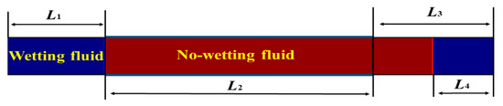
Figure 1.
Schematic figure of capillary imbibition.
Both wetting fluid and nonwetting fluid have the same density ρw = ρn = 1000 kg m−3. The viscosities are μw = 10 mPa·s and μn = 1 mPa·s, respectively. The interfacial tension is 0.04 N m−1. We show the position of meniscus varying with time for the given contact angle, fluids viscosities, and surface tension. The behavior of meniscus obtained by numerical method matches well with the theoretical solutions, as illustrated in Figure 2, which validates the correctness of the numerical model.

Figure 2.
The numerical and theoretical position of moving meniscus, and the analytical solution is Equation (11).
3.2. The Residual Oil Distribution under Different Wetting Conditions
In this section, a manufactured porous medium is used to investigate the residual oil distribution and formation mechanisms, as shown in Figure 3, Figure 4 and Figure 5. The size of this porous medium is 320 μm × 640 μm. The densities of oil and water are ρo = 890 kg m−3 and ρw = 1000 kg m−3. The viscosities of oil and water are μo = 15 mPa·s and μw = 1 mPa·s. The interfacial tension between two phases is 0.04 N m−1. The contact angles with the oil phase are 60°, 90°, and 120°, representing the oil-wet porous medium, neutral-wet porous medium, and water-wet porous medium, respectively. Initially, the porous medium is saturated with oil and water is injected from the left-hand side at an average velocity Uin = 0.04 m s−1. A pressure of 0 is set at the right-hand side as the outlet. The simulation is run until the oil saturation reaches a relatively steady state. The oil recovery rate of the porous medium and the water cut at the outlet are calculated and analyzed. Water cut is the ratio of water flow rate at the outlet to the total flow rate, and oil recovery rate is defined as the ratio of cumulative oil production to pore volume of the porous medium.
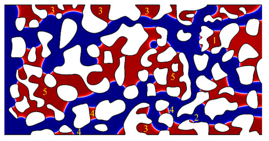
Figure 3.
Residual oil distribution in the oil-wet porous medium when the water cut is 98%. The white regions are rock matrix, and the red and blue regions represent oil and water, respectively. (1) isolated oil droplet; (2) oil film; (3) residual oil in dead ends; (4) residual oil in pore throats; and (5) cluster residual oil.

Figure 4.
Residual oil distribution in the neutral-wet porous medium when the water cut is 98%. The white regions are rock matrix, and the red and blue regions represent oil and water, respectively.
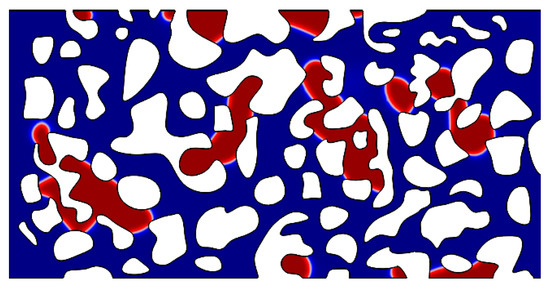
Figure 5.
Residual oil distribution in the water-wet porous medium when the water cut is 98%. The white regions are rock matrix, and the red and blue regions represent oil and water, respectively.
Zhu et al. [43] classified the residual oil as five categories: (1) isolated oil droplet, (2) oil film, (3) residual oil in dead ends, (4) residual oil in pore throats, and (5) cluster residual oil depending on the location and formation process of residual oil. Figure 3 shows the residual oil distribution in the oil-wet porous medium when the water cut is 98%. The white regions are rock matrix, while the red and blue regions represent oil and water, respectively. Different types of residual oil are marked by different numbers in Figure 3. However, there are some significant differences in the residual oil distribution in different wettability porous media. It is difficult to observe the existence of residual oil in pore throats and oil film in the neutral-wet and water-wet porous medium, as shown in Figure 4 and Figure 5. And the amount of residual oil in dead ends and cluster residual oil is dramatically reduced. As can be seen from these figures, wettability plays a fundamental role in determining the residual oil distributions. In order to understand the differences of residual oil distribution, it is essential to analyze the formation process and mechanism of residual oil.
The formations of residual oil in pore throats and oil film are dominated by the wettability of porous media. Oil is trapped on the wall and becomes oil film by the attractive force as hydrodynamic effect is weak during the flooding process. Consequently, the oil film is difficult to form when the pore wall is hydrophilic. As for residual oil in pore throats, capillary pressure is a primary factor in the formation process, which is closely related to the wettability. The remaining oil cannot be discharged from throats when the pressure difference is smaller than the maximum capillary pressure at the narrowest part of the pore throat. However, water is more likely to enter the small pore throat in the water-wet porous medium since capillary pressure is the driving force as water flows into pore throats.
Other types of residual oil are related to the rock structure. Cluster residual oil and residual oil in dead ends are two important types of residual oil, and rock structure plays an important role in their formation process. Rock structure is the main reason for the formation of residual oil in dead ends (marked 3 in Figure 3). The dead end is not a predominant pathway, which results in a low flow velocity of water and a poor sweep efficiency on oil, especially in the hydrophobic porous medium. In the water-wet porous medium, water can enter the dead end due to the capillary force when the water flow reaches a relatively steady state. Consequently, compared with the oil-wet porous medium, the volume of residual oil in dead ends in water-wet porous medium is lower. Unlike other types of residual oil, cluster residual oil exists in pore space in a continuous state, which means that reducing cluster residual oil is of great significance for EOR. A portion of the domain containing cluster residual oil is selected to analyze the formation process, as shown in Figure 6, which demonstrates that the heterogeneity of the porous medium is the major cause for the formation of cluster residual oil. Cluster residual oil is normally located in low-permeability zones, such as the micropores where radii of pores and throats are small. There are predominant pathways near the dense areas, as illustrated in Figure 6e. Water prefers to flow into large pores and displace oil due to the low entry pressure. Fingering phenomenon is clearly observed during this process because of the heterogeneity of porous media. Water bypasses the dense areas in a form of flowing around. Once a predominant pathway forms, the oil in dense zones is difficult to be swept. These two types of residual oil are both in the non-predominant pathway, and water cannot effectively sweep these areas because of specific rock structure. As for isolated oil droplet, the formation process is complicated and not controlled by a single factor, and therefore we have carefully analyzed the formation mechanism in another article [43]. To sum up, rock structure, wettability, and capillary pressure dominate the formation of residual oil.

Figure 6.
The formation process of cluster residual oil.
The difference in the residual oil distribution under different wetting conditions is also reflected in the oil recovery rates and water cut curves. Figure 7a shows the oil recovery rate (water saturation) in the porous medium during the flooding process. The oil recovery increases rapidly at the early stage at different wetting conditions. At 0.0045 s, the injection water breaks through the outlet almost at the same time due to the high injection velocity. The recovery rates show an obvious difference after water breaks through. For the oil-wet porous medium, the oil recovery increases slightly after water breakthrough and almost stops growing after 0.01 s. Nevertheless, for the neutral-wet and water-wet porous media, there is still a large amount of remaining oil being displaced at this stage. In the water-wet porous medium, capillary pressure is no longer the resistance of the injection water into the pores and throats. When the displacement pressure drops rapidly along the predominant pathway, water can still enter small pores and drive out the remaining oil under the action of small displacement pressure or capillary pressure. On the other hand, there is a resistance for imbibition of water in an oil-wet porous medium. Therefore, more oil is displaced out in the water-wet porous medium, which results in a lower residual oil saturation and a fall in water cut, as shown in Figure 7.

Figure 7.
The oil recovery and water cut at the outlet: (a) oil recovery rates (Y-axis is oil recovery rate, % and X-axis is time, s) and (b) water cut curves (Y-axis is water cut, % and X-axis is time, s).
Water cut has a vital impact on oil well production or reservoir development, which reflects the performance and potential of a well. Normally, 70% to 90% of water cut is called high water cut stage and oilfield development enters into an extra high water cut stage once water cut becomes over 90%. In general, the well or reservoir reaches the economic development limit and loses economic value when water cut rises to 98%. At the initial stage, only oil flows out from the outlet and water cut is zero, namely, the water-free oil production period. The development enters into water-oil production period when water breaks through at the outlet. After water breaking through the outlet, the water cut grows rapidly and reaches 90%. As can be seen from Figure 7b, the wettability of porous media exerts significant influence on water-oil production period. The raising rate of water cut slows down as the wettability changes from oil-wet to water-wet, and the economic lifetime of porous media is extended.
3.3. Pore-Scale Investigation of Enhancing Oil Recovery Methods
Increasing oil displacement efficiency and sweep efficiency is the key to recover residual oil effectively and enhance oil recovery. The emergence of surfactant flooding and polymer flooding has made it possible for oilfields to stabilize and increase production at high water cut stage [44]. In this section, the primary EOR mechanisms of surfactant and polymer flooding, as well as the process of reducing residual oil are investigated, including the effect of operation times on ultimate oil recovery. We choose the oil-wet porous medium (contact angle with the oil is 60°) as the research model. All simulations are run until oil saturation reaches a steady-state.
3.3.1. Investigation of Surfactant Flooding
In recent years, numerous studies have been conducted to investigate the EOR mechanisms of surfactant flooding and some important understanding have been elicited [45]. A crucial and direct element based on surfactant flooding is to reduce interfacial tension between aqueous and oil phases [23]. In this section, the effect of the surfactant solution on EOR is explored by decreasing the interfacial tension from 0.04 N m−1 to and 0.02 N m−1. Figure 8 demonstrates that decreasing interfacial tension by injecting the surfactant can enhance oil recovery significantly. The ultimate oil recovery increases by 9.0% as compared with water flooding. In addition, it takes more time to reach the steady-state for the case with a lower interfacial tension. A fall can be found in the water cut and the economic lifetime is extended as the surfactant flooding is implemented. For the water flooding case, the water cut reaches 98% at 0.009 s. Whereas for the surfactant flooding case, the water cut reaches 98% at 0.0125 s, which is 0.0035 s later than water flooding. The decline in water cut and the extension of economic development life mean that more remaining oil is produced, and the EOR mechanisms of surfactant flooding will be analyzed later. However, the application of surfactant flooding leads to the shortening of the water-free oil production period for oil-wet porous media. This is because the decrease of interfacial tension makes it easier for water to overcome entry pressure (capillary pressure) and occupy pore space, resulting in an increase in the average flow velocity of the injection fluid.

Figure 8.
Water cut at the outlet and oil recovery at different interfacial tensions (Y-axis is water cut, % and X-axis is time, s).
Selecting appropriate time of injecting the surfactant may have an important impact on oil recovery. To investigate this possible effect, the interfacial tension decreases from 0.04 N m−1 to and 0.02 N m−1 at the following five different times: t = 0 s (the initial stage of development), t = 0.005 s (water cut is about 90%), t = 0.01 s (the end of development, water cut is about 99%), t = 0.02 s (steady-state, water cut is about 100%), and t = 0.03 s (steady-state, water cut is about 100%). Results are presented in Figure 9a, obvious improvements in oil recovery can be observed as the surfactant flooding is applied at five different times, but the ultimate oil recovery rates are different. A higher ultimate recovery rate is obtained by injecting the surfactant before water flooding reaches stability. Compared with injection of the surfactant at the water-oil production period, water breaks through earlier at the outlet when the surfactant is applied at the initial stage, as shown in Figure 9b.

Figure 9.
The oil recovery and water cut at the outlet when the surfactant is injected at different times: (a) oil recovery rates (Y-axis is oil recovery rate, % and X-axis is time, s) and (b) water cut curves (Y-axis is water cut, % and X-axis is time, s).
Figure 10 presents the residual oil distributions with the surfactant applied at 0 s and 0.03 s. Comparing the residual oil distributions after water flooding (Figure 3) and surfactant flooding (Figure 10a), we find that displacement efficiency is improved in surfactant flooding and some oil retained in the corner of pore throats after water flooding is displaced. It is also interesting to find that some regions that are not swept in water flooding due to heterogeneity of the porous medium are affected by surfactant solutions, which implies that surfactant flooding could increase microscale sweep efficiency to some extent. This phenomenon is attributed to the lower capillary force which reduces the entry pressure of micropores.

Figure 10.
Residual oil distributions when the surfactant is injected at different times: (a) surfactant is injected at 0 s and (b) surfactant is injected at 0.03 s.
However, there are some remarkable differences in residual oil distributions when the surfactant is injected at different times, as shown in the circled part of Figure 10. To observe the differences in residual oil distribution clearly and explore the mechanisms, a circled part is selected to analyze this process. Figure 11 compares the pressure difference between a and b with the surfactant applied at 0 s and 0.03 s, respectively. For the 0 s case, the pressure difference between a and b is much higher than maximum capillary pressure when the pore throat has not been swept by water. At 0.0019 s, the water-oil interface reaches point a on the side of the throat, as illustrated in Figure 11a. At this time, the pressure between a and b is still higher than the maximum capillary pressure. The pressure difference drops rapidly when water spreads to b, with the formation of water-flow pathway. While for the 0.03 s case, the pressure difference between these two points is only a little larger than the maximum capillary pressure when the water spreads to point a. However, the flow pressure decreases with the high-permeability pathway in the direction of the yellow arrow, as illustrated in Figure 11b, and the pressure difference between a and b declines immediately. At 0.03 s, the maximum capillary pressure decreases with the application of the surfactant. But the displacement pressure is still not high enough to “push” water pass through the throat due to the formation of predominant pathway alongside. This situation is related to the rock structure used in this research, while such rock structure is ubiquitous in real reservoirs. In addition, the water flooding may reach stability in some high-permeability regions of the reservoir when the water cut at production wells is high. Although some effects of surfactant flooding are neglected in this study, to the best of our knowledge, surfactants cannot restrain the formation of predominant pathway. Consequently, applying surfactant flooding at the low water cut stage is a suitable case to obtain higher ultimate oil recovery.

Figure 11.
The pressure difference between a and b when the surfactant is injected at different times: (a) surfactant is injected at 0 s and (b) surfactant is injected at 0.03 s.
To sum up, the low interfacial tension produced by surfactant flooding, not only improves oil displacement efficiency, but also increases microscale sweep efficiency by reducing the entry pressure of micropores. This mechanism does not inhibit the formation of predominant pathway, so it leads to the difference in the ultimate oil recovery of different operation times. Once the high-permeability pathway of water flow forms and remains stable, the effects of surfactant flooding can be compromised, especially for the remaining oil in dense zones. Injecting the surfactant solution before water flooding reaches a steady-state can obtain a higher ultimate oil recovery.
3.3.2. Investigation of Polymer Flooding
Polymer flooding is another common practice for EOR in oilfields. In this section, the EOR mechanisms of polymer flooding and effect of operation times on oil recovery are studied. Note that the elasticity of the polymer is not considered in this study; only the viscous effect is taken into account. The primary effect of polymer flooding is to increase the viscosity of displacement fluid, as a first-order address to the problem of unstable displacement. The viscosity of displacement fluid increases from 1 mPa·s to 15 mPa·s to investigate the effect of polymer flooding on EOR. Figure 12 shows the water cut at the outlet and oil recovery in the porous medium when the displacement fluid viscosities are 1 mPa·s and 15 mPa·s, respectively. Consistent with the development experience of oilfield, the oil recovery is improved dramatically with the increase of displacement fluid viscosity. Water cut experiences a considerable decline as compared with the water flooding, implying more oil is produced at the water-oil production period. At 0.04 s, water cut rises to 99.29% and oil left in the porous medium is trapped permanently.

Figure 12.
Water cut at the outlet and oil recovery at different displacement fluid viscosities (Y-axis is water cut, % and X-axis is time, s).
Figure 13 compares the displacement processes in water flooding and polymer flooding. In water flooding, relatively obvious and long fingers of injectant can be observed, leading to a lower oil recovery and early water breaking through. With the increase of displacement fluid viscosity in polymer flooding, the fingering phenomenon is less remarkable and the absolute length of viscos fingers also reduces. As a result, the displacement front is spatially more uniform and appears to be relatively stabilized at a larger scale observation. In terms of residual oil distributions, on the one hand, water flooding exhibits viscous fingers which propagate through the porous medium leaving large cluster residual oil behind, and the heterogeneities of the porous medium exacerbate this phenomenon. On the other hand, the sweep efficiency is dramatically improved in polymer flooding, contributing to a decline in cluster residual oil and the residual oil is scattered with occupancy of the smaller pores. In contrast, some residual is still continuous and occupies large pore throats after water flooding.

Figure 13.
Displacement processes in water flooding and polymer flooding (μ = 15 mPa·s): (a) water flood t = 0.002 s, (b) water flood t = 0.003 s, (c) water flood t = 0.0045 s, (d) water flood t = 0.04 s, (e) polymer flood t = 0.002 s, (f) polymer flood t = 0.003 s, (g) polymer flood t = 0.0045 s, and (h) polymer flood t = 0.04 s.
Then, the appropriate injection time of the polymer solution is also investigated. The viscosity of displacement fluid increases from 1 mPa·s to 15 mPa·s at the following five different times: t = 0 s, t = 0.005 s, t = 0.01 s, t = 0.02 s, and t = 0.03 s. Figure 14 illustrates that ultimate oil recoveries are basically identical as the polymer is injected at different times, although water cut curves show some differences. Among these schemes, more oil is produced during the water-free oil production period as polymer flooding is used at the initial stage of development. However, the operation time of polymer flooding does not exert significant influence on the ultimate recovery, which differs from surfactant flooding. In order to investigate the mechanism of this phenomenon, the force analysis of two-phase fluids flowing in pore throats is performed, as shown in Figure 15. The following three forces mainly affect the movement of the two-phase interface in this model: viscous force (, resistance), displacement force (, motive power), and capillary force (, depending on the wettability of porous media). Notably, gravity is not considered in this study. If the rate of motive powers to resistances (RMR) is greater than unity, the displacement fluid can drive the oil forward. When the two-phase interface in a single throat moves to divergent throats, the RMRs in divergent throats are different because of the variations in capillary force between diverse sizes of throats. The displacement fluid tends to enter the throat with less resistance as the difference of RMRs in divergent throats reaches a threshold, and the fingering phenomenon appears in divergent throats. Subsequently, the displacement pressure falls dramatically along the bigger throat and is not big enough to “push” the oil forward in the smaller throat.

Figure 14.
The oil recovery and water cut at the outlet when the polymer solution is injected at different times: (a) oil recovery rates (Y-axis is oil recovery rate, % and X-axis is time, s) and (b) water cut curves (Y-axis is water cut, % and X-axis is time, s).
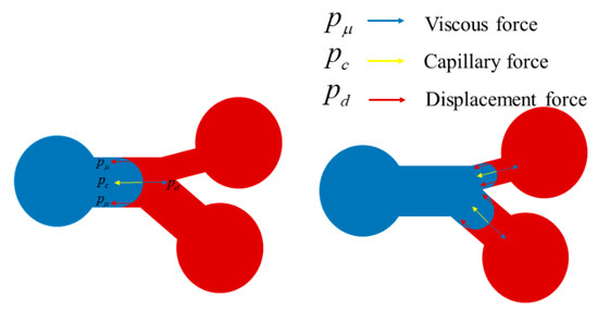
Figure 15.
Force analysis of fluids flowing through pore throat.
The implementation of polymer flooding increases the viscous force of fluids flow in porous media. As can be seen in Table 1, viscous force is always the resistance, and the difference of RMRs in divergent throats reduces with an increase of viscous force in oil-wet as well as in water-wet porous media. In other words, viscous force takes a more important position as the viscosity of displacement fluid increases. The increase in viscous force weakens the effect of capillary force. As a result, the displacement fluid tends to enter the throats with different sizes uniformly, which leads to the improvement in sweep efficiency in macroscopic. This characteristic of polymer flooding prevents the formation of high-permeability pathway. Therefore, the effect of polymer flooding does not show the obvious time-dependent effect like surfactant flooding.

Table 1.
The changing trend of the difference of rate of motive powers to resistances (RMRs) in divergent throats with the increase of displacement fluid viscosity.
4. Conclusions
In this study, a direct numerical method coupled with a phase field method is firstly used to investigate the distribution of residual oil at high water cut stage and the mechanisms of EOR methods. Appropriate application times and potentials of surfactant flooding and polymer flooding are studied at the pore scale. The simulation results show that:
- The distributions of residual oil in porous media are significantly different under different wetting conditions. Rock structure, wettability, and capillary pressure dominate the formation of residual oil.
- The wettability of porous media exerts significant influence on the water-oil production period. The raising rate of water cut slows down when the wettability changes from oil-wet to water-wet, and the economic lifetime of porous media is extended.
- The surfactant flooding not only improves oil displacement efficiency, but also increases microscale sweep efficiency by reducing the entry pressure of micropores. The injection time of the surfactant solution exerts an important influence on the ultimate oil recovery because of the formation of predominant pathway. Implementing surfactant flooding at the low water cut stage is a suitable case to obtain higher ultimate oil recovery.
- Polymer flooding improves oil sweep efficiency by reducing the difference of RMRs in divergent throats and weakening the effect of capillary force. The displacement front is spatially more uniform with a later breakthrough as compared with water flooding. There is no significant correlation between ultimate recovery of polymer flooding and its injection time.
In addition, the direct numerical method coupling with a phase field method can be used to investigate the residual oil distribution and EOR mechanisms at the pore-scale model level. Compared with microscopic visualization experiments, micro-numerical simulation can save experimental expenses and avoid complex experimental operations in sensitivity analysis. However, changing viscosity and interfacial tension is a simplified situation of polymer flooding and surfactant flooding. How to consider the adsorption problem and other flow characteristics of polymer and surfactant flooding still needs further investigations.
Supplementary Materials
The following are available online at https://www.mdpi.com/1996-1073/12/19/3732/s1.
Author Contributions
Investigation, H.S., W.S. and Y.Y.; Methodology, G.Z.; Validation, J.Y.; Writing—original draft, Y.G.; Writing—review & editing, L.Z., J.Y. and J.Z.
Funding
This work was financially supported by National Natural Science Foundation of China (No.51490654, No.51504276, No.51674280 and No.51711530131), Shandong Provincial Natural Science Foundation (ZR2019JQ21), Fundamental Research Funds for the Central Universities (No.18CX02031A and No. 17CX05003), Key Research and Development Plan of Shandong Province (2018GSF116009).
Acknowledgments
The authors thank the anonymous reviewers and all the editors in the process of manuscript revision.
Conflicts of Interest
The authors declare no conflict of interest.
References
- Hajirezaie, S.; Wu, X.; Peters, C.A. Scale formation in porous media and its impact on reservoir performance during water flooding. J. Nat. Gas Sci. Eng. 2017, 39, 188–202. [Google Scholar] [CrossRef]
- Shedid, S.A. Influences of fracture orientation on oil recovery by water and polymer flooding processes: An experimental approach. J. Pet. Sci. Eng. 2006, 50, 285–292. [Google Scholar] [CrossRef]
- Cheng, J.; Wu, J.; Hu, J. Key theories and technologies for enhanced oil recovery of alkaline/surfactant/polymer flooding. Acta Pet. Sin. 2014, 35, 310–318. [Google Scholar]
- Mojarad, R.; Settari, A. Velocity-based formation damage characterization method for produced water re-injection: Application on masila block core flood tests. Pet. Sci. Technol. 2008, 26, 937–954. [Google Scholar] [CrossRef]
- Jaramillo, O.J.; Romero, R.; Lucuara, G.; Ortega, A.; Milne, A.W.; Lastre Buelvas, M. Combining stimulation and water control in high-water-cut wells. In Proceedings of the SPE International Symposium and Exhibition on Formation Damage Control, Lafayette, LA, USA, 10–12 February 2010; pp. 1–10. [Google Scholar]
- Song, Z.; Li, Z.; Lai, F.; Liu, G.; Gan, H. Derivation of water flooding characteristic curve for high water-cut oilfields. Pet. Explor. Dev. 2013, 40, 216–223. [Google Scholar] [CrossRef]
- Zhang, L.; Jing, W.; Yang, Y.; Yang, H.; Guo, Y.; Sun, H.; Zhao, J.; Yao, J. Investigation of Permeability Calculation Using Digital Core Simulation Technology. Energies 2019, 12, 3273. [Google Scholar] [CrossRef]
- Sheng, J. Enhanced oil recovery in shale reservoirs by gas injection. J. Nat. Gas Sci. Eng. 2015, 22, 252–259. [Google Scholar] [CrossRef]
- Cai, J.; Zhang, Z.; Kang, Q.; Harpteet, S. Recent Advances in Flow and Transport Properties of Unconventional Reservoirs. Energies 2019, 12, 1865. [Google Scholar] [CrossRef]
- Alvarado, V.; Manrique, E. Enhanced Oil Recovery: An Update Review. Energies 2010, 3, 1529–1575. [Google Scholar] [CrossRef]
- Gan, L.; Dai, X.; Zhang, X.; Li, L.; Du, W.; Liu, X.; Gao, Y.; Liu, M.; Ma, S.; Huang, Z. Key technologies for seismic reservoir characterization of high water-cut oilfields. Pet. Explor. Dev. 2012, 39, 391–404. [Google Scholar] [CrossRef]
- Yang, Y.; Yang, H.; Tao, L.; Yao, J.; Wang, W.; Zhang, K.; Luquot, L. Microscopic determination of remaining oil distribution in sandstones with different permeability scales using CT-scanning. J. Energy Resour. Technol.-Trans. ASME 2019, 141, 092903. [Google Scholar] [CrossRef]
- Iglauer, S.; Fernø, M.; Shearing, P.; Blunt, M. Comparison of residual oil cluster size distribution, morphology and saturation in oil-wet and water-wet sandstone. J. Colloid Interface Sci. 2012, 375, 187–192. [Google Scholar] [CrossRef] [PubMed]
- Yan, X.; Huang, Z.; Yao, J.; Li, Y.; Fan, D. An efficient embedded discrete fracture model based on mimetic finite difference method. J. Pet. Sci. Eng. 2016, 145, 11–21. [Google Scholar] [CrossRef]
- Cai, J.; Yu, B. A Discussion of the Effect of Tortuosity on the Capillary Imbibition in Porous Media. Transp. Porous Media 2011, 89, 251–263. [Google Scholar] [CrossRef]
- Chen, Y.; Fang, S.; Wu, D.; Hu, R. Visualizing and quantifying the crossover from capillary fingering to viscous fingering in a rough fracture. Water Resour. Res. 2017, 53, 7756–7772. [Google Scholar] [CrossRef]
- Meng, Q.; Xu, S.; Cai, J. Microscopic studies of immiscible displacement behavior in interconnected fractures and cavities. J. Energy Resour. Technol. Trans. ASME 2019, 141, 092901. [Google Scholar] [CrossRef]
- Wu, K.; Van Dijke, M.I.; Couples, G.D.; Jiang, Z.; Ma, J.; Sorbie, K.S.; Crawford, J.; Young, I.; Zhang, X. 3D stochastic modelling of heterogeneous porous media–applications to reservoir rocks. Transp. Porous Media 2006, 65, 443–467. [Google Scholar] [CrossRef]
- Yang, Y.; Liu, Z.; Yao, J.; Zhang, L.; Ma, J.; Hejazi, S.; Luquot, L.; Ngarta, T. Flow simulation of artificially induced microfractures using digital rock and lattice Boltzmann methods. Energies 2018, 11, 2145. [Google Scholar] [CrossRef]
- Kumar, M.; Knackstedt, M.A.; Senden, T.J.; Sheppard, A.P.; Middleton, J.P. Visualizing and quantifying the residual phase distribution in core material. Petrophysics 2010, 51, 323–332. [Google Scholar]
- Gao, H.; Liu, Y.; Zhang, Z.; Niu, B.; Li, H. Impact of secondary and tertiary floods on microscopic residual oil distribution in medium-to-high permeability cores with NMR technique. Energy Fuels 2015, 29, 4721–4729. [Google Scholar] [CrossRef]
- Jamaloei, B.Y.; Kharrat, R. Analysis of microscopic displacement mechanisms of dilute surfactant flooding in oil-wet and water-wet porous media. Transp. Porous Media 2010, 81, 1–19. [Google Scholar] [CrossRef]
- Ahmadi, M.A.; Shadizadeh, S.R. Implementation of a high-performance surfactant for enhanced oil recovery from carbonate reservoirs. J. Pet. Sci. Eng. 2013, 110, 66–73. [Google Scholar] [CrossRef]
- Souza, F.M.; Nandenha, J.; Batista, B.L.; Oliveira, V.H.A.; Pinheiro, V.S.; Parreira, L.S.; Neto, A.O.; Santos, M.C. Pd x Nb y electrocatalysts for DEFC in alkaline medium: Stability, selectivity and mechanism for EOR. Int. J. Hydrogen Energy 2018, 43, 4505–4516. [Google Scholar] [CrossRef]
- Lu, C.; Zhao, W.; Liu, Y.; Dong, X. Pore-scale transport mechanisms and macroscopic displacement effects of in-situ Oil-in-Water emulsions in porous media. J. Energy Resour. Technol.-Trans. ASME 2018, 140, 102904. [Google Scholar] [CrossRef]
- Buchgraber, M.; Clemens, T.; Castanier, L.M.; Kovscek, A. A microvisual study of the displacement of viscous oil by polymer solutions. SPE Reserv. Eval. Eng. 2011, 14, 269–280. [Google Scholar] [CrossRef]
- Dong, M.; Ma, S.; Liu, Q. Enhanced heavy oil recovery through interfacial instability: A study of chemical flooding for Brintnell heavy oil. Fuel 2009, 88, 1049–1056. [Google Scholar] [CrossRef]
- Rodríguez, D.C.A.; Oostrom, M.; Shokri, N. Effects of shear-thinning fluids on residual oil formation in microfluidic pore networks. J. Colloid Interface Sci. 2016, 472, 34–43. [Google Scholar] [CrossRef]
- Bera, A.; Mandal, A.; Guha, B. Synergistic effect of surfactant and salt mixture on interfacial tension reduction between crude oil and water in enhanced oil recovery. J. Chem. Eng. Data 2013, 59, 89–96. [Google Scholar] [CrossRef]
- Maghzi, A.; Kharrat, R.; Mohebbi, A.; Ghazanfari, M.H. The impact of silica nanoparticles on the performance of polymer solution in presence of salts in polymer flooding for heavy oil recovery. Fuel 2014, 123, 123–132. [Google Scholar] [CrossRef]
- Wang, S.; Feng, Q.; Dong, Y.; Han, X.; Wang, S. A dynamic pore-scale network model for two-phase imbibition. J. Nat. Gas Sci. Eng. 2015, 26, 118–129. [Google Scholar] [CrossRef]
- Peszynska, M.; Trykozko, A. Pore-to-core simulations of flow with large velocities using continuum models and imaging data. Comput. Geosci. 2013, 17, 623–645. [Google Scholar] [CrossRef]
- Tryggvason, G.; Bunner, B.; Esmaeeli, A.; Juric, D.; Al-Rawahi, N.; Tauber, W.; Han, J.; Nas, S.; Jan, Y. A front-tracking method for the computations of multiphase flow. J. Comput. Phys. 2001, 169, 708–759. [Google Scholar] [CrossRef]
- Guo, Y.; Zhang, L.; Yao, J.; Sun, H.; Yang, Y.; Huang, T. Mechanisms of water flooding characteristic curve upwarping at high water-cut stage and influencing factors. Chin. Sci. Bull. 2019, 64. [Google Scholar] [CrossRef]
- Graveleau, M.; Soulaine, C.; Tchelepi, H.A. Pore-scale simulation of interphase multicomponent mass transfer for subsurface flow. Transp. Porous Media 2017, 120, 287–308. [Google Scholar] [CrossRef]
- Enright, D.; Fedkiw, R.; Ferziger, J.; Mitchell, I. A hybrid particle level set method for improved interface capturing. J. Comput. Phys. 2002, 183, 83–116. [Google Scholar] [CrossRef]
- Villanueva, W.; Amberg, G. Some generic capillary-driven flows. Int. J. Multiph. Flow 2006, 32, 1072–1086. [Google Scholar] [CrossRef]
- Gunde, A.C.; Bera, B.; Mitra, S.K. Investigation of water and CO2 (carbon dioxide) flooding using micro-CT (micro-computed tomography) images of Berea sandstone core using finite element simulations. Energy 2010, 35, 5209–5216. [Google Scholar] [CrossRef]
- Boyer, F.; Lapuerta, C.; Minjeaud, S.; Piar, B.; Quintard, M. Cahn–Hilliard/Navier–Stokes model for the simulation of three-phase flows. Transp. Porous Media 2010, 82, 463–483. [Google Scholar] [CrossRef]
- Zhou, C.; Yue, P.; Feng, J.; Ollivier-Gooch, C.F.; Hu, H. 3D phase-field simulations of interfacial dynamics in Newtonian and viscoelastic fluids. J. Comput. Phys. 2010, 229, 498–511. [Google Scholar] [CrossRef]
- Zhu, G.; Chen, H.; Yao, J.; Sun, S. Efficient energy-stable schemes for the hydrodynamics coupled phase-field model. Appl. Math. Model. 2019, 70, 82–108. [Google Scholar] [CrossRef]
- Liu, H.; Valocchi, A.J.; Werth, C.; Kang, Q.; Oostrom, M. Pore-scale simulation of liquid CO2 displacement of water using a two-phase lattice Boltzmann model. Adv. Water Resour. 2014, 73, 144–158. [Google Scholar] [CrossRef]
- Zhu, G.; Yao, J.; Zhang, L.; Sun, H.; Li, A.; Zhang, K. Pore-scale investigation of residual oil distributions and formation mechanisms at the extra-high water-cut stage. Chin. Sci. Bull. 2017, 62, 2553–2563. [Google Scholar] [CrossRef]
- Abidin, A.Z.; Puspasari, T.; Nugroho, W.A. Polymers for enhanced oil recovery technology. Procedia Chem. 2012, 4, 11–16. [Google Scholar] [CrossRef]
- Wang, Z.; Yu, T.; Lin, X.; Wang, X.; Su, L. Chemicals loss and the effect on formation damage in reservoirs with ASP flooding enhanced oil recovery. J. Nat. Gas Sci. Eng. 2016, 33, 1381–1389. [Google Scholar] [CrossRef]
© 2019 by the authors. Licensee MDPI, Basel, Switzerland. This article is an open access article distributed under the terms and conditions of the Creative Commons Attribution (CC BY) license (http://creativecommons.org/licenses/by/4.0/).