Article

The Distinct Elemental Analysis of the Microstructural Evolution of a Methane Hydrate Specimen under Cyclic Loading Conditions

1
State Key Laboratory of Mining Disaster Prevention and Control, Shandong University of Science and Technology, Qingdao 266590, China
2
Department of Geotechnical Engineering, Graduate School of Engineering, Nagasaki University, Nagasaki 852-8521, Japan
*
Author to whom correspondence should be addressed.
These authors contributed to the work equally and should be regarded as co-first authors.
Energies 2019, 12(19), 3694; https://doi.org/10.3390/en12193694
Submission received: 3 August 2019 / Revised: 12 September 2019 / Accepted: 23 September 2019 / Published: 27 September 2019

Abstract

:
Submarine slope instability may be triggered by earthquakes and tsunamis. Methane hydrate sediments (MHS) are commonly buried under submarine slopes. Submarine slides would probably be triggered once the MHS are damaged under cyclic loading conditions. For this reason, it is essential to research the mechanical response of MHSs under dynamic loading conditions. In this study, a series of drained cyclic biaxial compressive tests with constant stress amplitudes were numerically carried out with the distinct element method (DEM). The cyclic loading number decreased as the hydrate saturation (Sh) increased when the MHS were damaged. The failure mode of the MHS was shown to be dependent on the dynamic stress amplitude and hydrate saturation. The microstructure of MHS during the cyclic loading shear process was also analyzed. The results can help us to understand the mechanical behavior of MHS during the cyclic loading process and develop micromechanical-based constitutive models.

Graphical Abstract

1. Introduction

Methane hydrate is ice-like solid energy, which is generally founded in the subpermafrost and deep seabed where the pressure is high and the temperature is low. In order to extract methane gas from the methane hydrate sediment, the methane hydrate needs to be dissociated first. Methane hydrates are very sensitive to the occurrence environment and can be dissociated when the pressure decreases and/or the temperature increases. There are three main production techniques including thermal injection, chemical injection, and depressurization. Due to the environmental sensitivity of methane hydrates, the extraction of methane hydrates from seabed sediments may create a geohazard. In order to mine methane hydrates safely, the mechanical properties of methane hydrate-bearing sediments (MHS) should be studied.
The mechanical properties of MHS have been researched by using various methods, including in situ tests, synthetic sediment tests, and simulated tests. The in situ tests can reveal the mechanical properties of MHS precisely. In previous decades, there were several methane hydrate gas production tests of methane hydrates conducted around the world. The Messoyakha gas hydrate deposit was discovered in 1967. The production of methane gas production began in December 1969 [1]. Japan, Canada, and the United States conducted pressure drawdown tests using Schlumberger’s Modular Formation Dynamics Tester (MDT) in the Millik methane hydrate reservoirs in 2002, and in the Mount Elbert methane hydrate reservoirs in 2007 [2]. In 2013, offshore methane hydrate gas production was first conducted in the Eastern Nankai Trough, Japan [3]. From April to June 2017, Japan conducted the second extraction test of methane hydrates in the Eastern Nankai Trough [4]. From May to July 2017, China tested the production of methane hydrate gas from MHS in the South China Sea [5]. In May 2017, China investigated the extraction of methane hydrates using the solid fluidization method [6]. Based on these extraction tests, a series of in situ mechanical property tests were conducted on MHS. Winters et al. [7] conducted triaxial shear tests of field sediments drilled from the Mackenzie Delta. Priest et al. [8] tested the mechanical properties of MHS drilled in the Eastern Nankai Trough using the PCATS Triaxial. The properties discovered included a small strain stiffness, stress–strain properties (triaxial shear tests), and permeability. Yoneda et al. [9,10] conducted undrained/drained compression tests and isotropic loading and unloading tests to test the in situ mechanical properties of MHS in the Eastern Nankai Trough. Priest et al. [11] conducted undrained triaxial shear tests using in situ sediment from the Indian National Gas Hydrate Program (NGHP). They found that the sediments have low shear strength, and hydrate is the main factor contributing to the improved strength of sediments. In the aforementioned in situ tests of the mechanical properties of MHS, the shear strength of MHS increased as the methane hydrate saturation (Sh) increased. Methane hydrate saturation refers to the volume percentage of methane hydrates in the spaces among soil particles.
Because the in-situ tests of MHS are costly and advanced techniques are needed, most of the mechanical property tests of MHS were conducted in the laboratory by using synthetic sediments. In previous research, the mechanical properties of MHS were tested by using direct shear tests, triaxial compressive tests, and bending tests. Masui et al. [12], Miyazaki et al. [13,14], and Hyodo [15,16,17,18,19] tested the triaxial compressive properties of synthetic methane hydrate sediments. In their studies, the shear strength and stiffness of MHS increased with an increasing Sh. Miyazaki et al. [20] also tested the strain rate effect on the strength of MHS. In their research, the strength of MHS increased as the strain rate increased. The strain rate dependence of MHS is as strong as that of frozen sand. Li et al. [21] conducted a series of triaxial tests to investigate the mechanical properties of MHS under different mining methods. In their research, the stability of MHS decreased under depressurization and heating conditions. Liu et al. [22] proposed an efficient method to evaluate the mechanical properties of MHS. Their test results indicated that hydrate strengthens specimens by cementing silt grains. Kajiyama et al. [23,24] tested the effects of particle characteristics on the mechanical response of MHS using compressive tests. Gong [25] tested the mechanical properties of MHS in the laboratory using a multiple failure test method. The mechanical properties of MHS were studied from different aspects in the above tests using various test apparatuses and methods. The test results indicate that the mechanical properties of MHS significantly depend on the hydrate saturation.
In general, most of the research on the mechanical properties of MHS has focused on statics analysis. In reality, MHS would be subject to the effects of dynamic loading, including seismic loading and wave loading. One of the largest known submarine slides is the Storegga Slide, as shown in Figure 1 [26]. The triggering mechanism is a combination of different effects; e.g., methane hydrate dissociation and earthquakes [27,28]. For this reason, it is essential to research the mechanical response of MHS under dynamic loading conditions. The Aitape earthquake in Papua New Guinea resulted in one of the largest submarine slope failures caused by a large earthquake, and a large tsunami [29,30]. The Kocaeli earthquake in Turkey triggered slope instability and movement [31]. The slope sliding triggered by the Aitape and Kocaeli earthquakes illustrates the close association between earthquakes, tsunamis, and slope failures. If slope instability is associated with a tsunami and/or an earthquake, it is possible that the MHS discovered in the slope are more easily damaged under dynamic loading conditions. Clayton et al. [32] tested the effects of the existence of methane hydrate on the shear modulus, bulk modulus, and the damping of MHS by using a modified Stoke-resonant column apparatus. Priest et al. [33] studied the effect of methane hydrate’s existence on the compressional wave and shear wave velocities using remote seismic methods. Kingston et al. [34] investigated the dynamic characteristics of MHS, such as the compressional wave velocity, shear wave velocity, and their respective attenuation characteristics, considering the particle sizes and shapes. Lee et al. [35] studied the effects of particle types such as sand, silts, and clay, with and without hydrate, on the compressional waves and shear velocities. Zhang et al. [36] conducted a series of dynamic triaxial tests on artificial MHS. In their studies, the number of cycles to failure was significantly affected by the dynamic loading amplitude; and the dynamic strength increased as the confining pressure decreased, and decreased as the temperature increased. The dynamic response of MHS has been studied, but the mechanism responsible for the response is not clear.
In recent years, soil fabric has been broadly used to describe arrangements of particles, contacts, and other anisotropic parameters during the cyclic loading process. However, only the macroscopic behaviors of specimens can be captured with conventional laboratory techniques. It is very time-consuming and technically difficult to measure the soil fabric and monitor its evolution when the specimen is loading. Alternatively, fabric evolution can be numerically simulated by the distinct element method (DEM) [37]. The DEM has been broadly used to investigate the mechanical responses of soils and rocks, which include the cyclic behaviors of soils. Previous studies have confirmed that the cyclic behaviors of soil can be successfully evaluated by the DEM.
The main purpose of the present work is to obtain a better understanding of the microstructure evolution of MHS under cyclic loading and to aid in the development of micromechanical-based constitutive models. To achieve this aim, a series of drained cyclic biaxial compressive tests with constant stress amplitudes were numerically carried out with DEM considering the cementing of hydrate particles and the rolling resistance among particles.

2. Numerical MHS Models with Different Levels of Hydrate Saturation

2.1. Particle Flow Code (PFC)

Cundall and Strack [37] proposed the particle flow code (PFC) theory in 1979. This theory is based on the DEM. The material particles are assumed to be disks of unit thickness (PFC2D) or balls (PFC3D) which are considered rigid and have normal and tangential stiffness. Among the disks or balls, contact models are activated. In this work, the numerical MHS was simulated by using disks, the rolling resistance model (RRM), and the parallel bond contact model (PBM) (Itasca consult group Inc. 2014). The RRM (Figure 2a) has rolling resistance friction and sliding resistance friction to resist the particle rotation or slide. The PBM (Figure 2b) can resist such particle movements, since PBM acts like a beam that resists the bending moment occurring within the bonded area [38]. The bond stiffness will lose its effect when the bond is broken. In this study, the PBM was assembled between the soil particles and hydrate particles, while the RRM was assembled among the soil particles. The default contact model among the particles was set to the RRM when the PBM was broken.

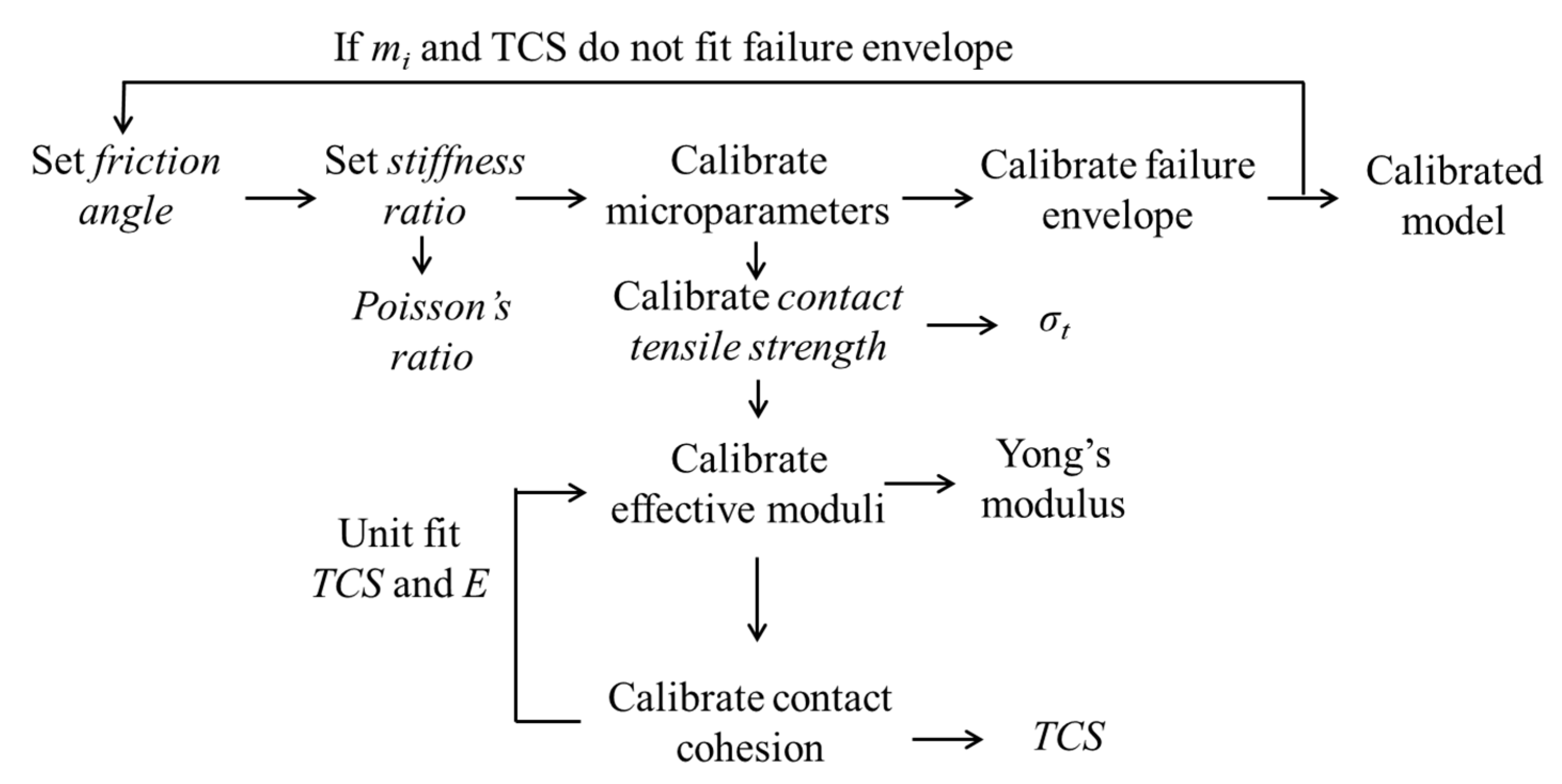
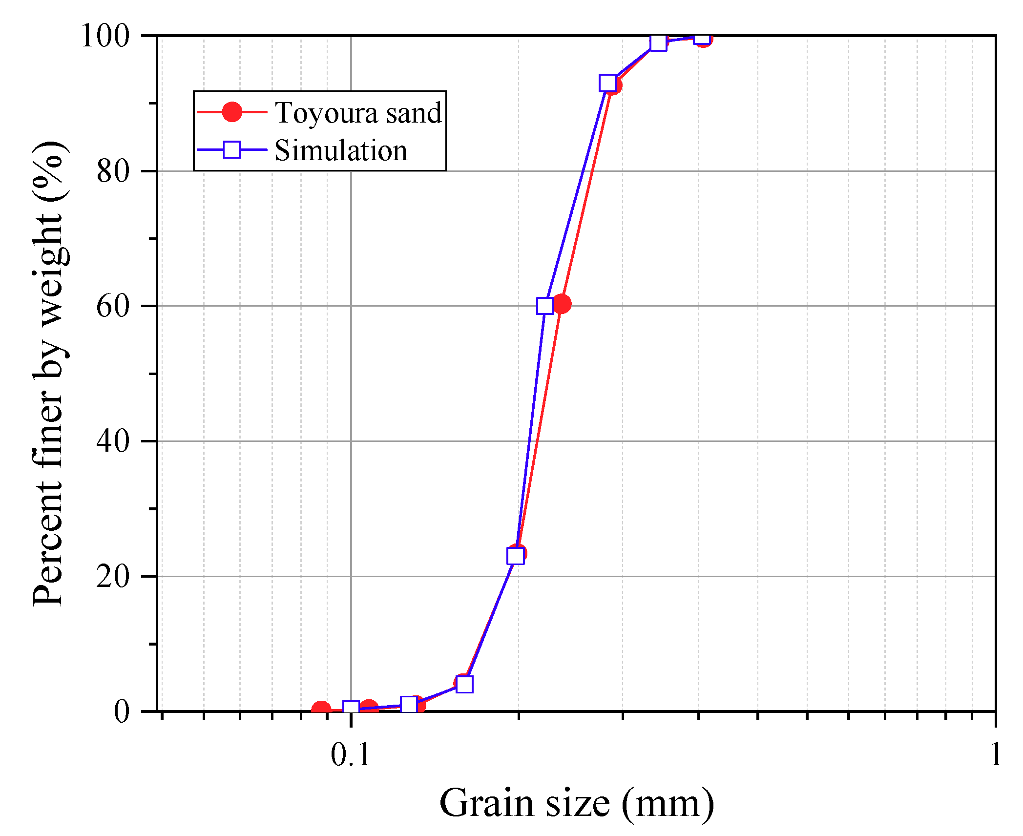
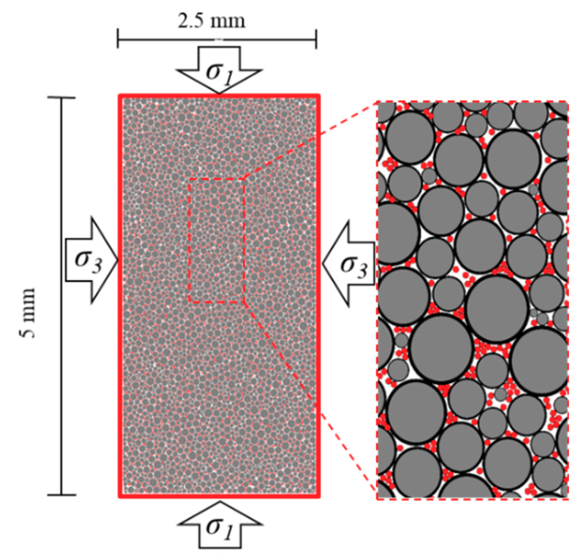
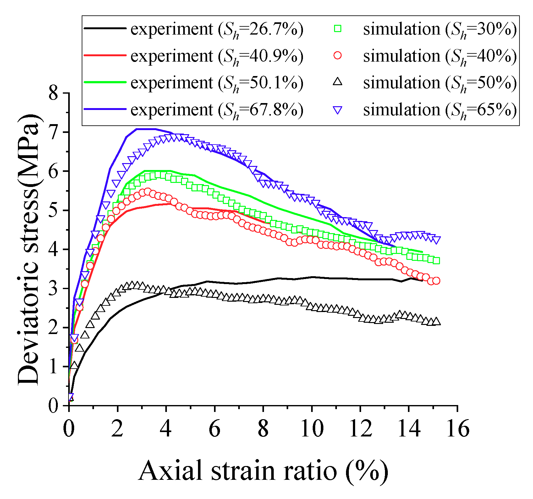
2.2. Parameter Checking and the Verification of MHS

The microscopic mechanical parameters of the particles and the contact model parameters must be set prior to running numerical simulation tests using the PFC. However, these parameters cannot directly be acquired from laboratory tests. Therefore, the microscopic parameters of particles and contact models must be selected and verified before the numerical simulations. When selecting the parameters, a large number of numerical simulation tests were first conducted under similar test conditions to the laboratory tests or in situ tests. Then, the numerical simulation results were compared with the results of experimental tests or field tests. The microscopic mechanical parameters were adjusted repeatedly by the “trial and error” method [39] until they met the required simulation conditions. The “trial and error” method used to check the PFC simulation process (version 5.0) is shown in Figure 3.
PFC3D can simulate the experimental triaxial testing of specimens. When the specimen is of cylindrical shape, the confining pressure is a constant value. Hence, the shear tests can be simulated by using PFC2D. Many researchers have used PFC2D to calculate the mechanical properties of geomaterials [40,41]. In this work, the initial size of the test specimens was set to 5 mm by 2.5 mm in height and in width, respectively. According to the particle-size distribution of soil used in the experimental tests (see Figure 4) [42], 3500 balls with diameters ranging from 0.1 mm to 0.4 mm were generated in a rectangular region with rigid, frictionless walls. The initial porosity was set to 0.1, and the inter-friction value was set to 0.5. After the numerical specimen was generated, the specimen was compressed by a numerical servo-control mechanism until the specimen reached the desired isotropic stress state (0.5 MPa).
Considering the deep-submarine generation of MHS, it is assumed that hydrates are formed after initial geostatic stresses to the soil skeleton. During the whole experimental test process, the specimen was conducted in a low-temperature environment. To prepare the test specimen, Toyuora sand and ice powder (the diameter is less than 250 μm) were mixed, with a target sand ratio (the percent of sand mass in the total mass of sand and ice, SMR). The mixture of sand and ice powder was consolidated to be a cylindrical shape measuring 50 mm in diameter and 200 mm in height, and the mixture was transferred into the pressure room of the test apparatus. Methane gas was injected into the mixture after the ice powder was melted into water. When the pressure of methane gas is maintained at a constant, methane hydrate has been generated in the pores among soil particles [25]. In the numerical simulation, first, the positions of walls and soil particles were fixed, and the diameters of soil particles were shrunk to one-tenth of their original values. Methane hydrate particles were randomly generated in the pore among soil particles, following which, soil particles were freed and expanded to their original diameter. In order to simulate the cementation of methane hydrate, the parallel-bond contact model was set onto the contact point in which a hydrate particle existed. Considering the rolling of particles, the rolling resistance model was applied to determine soil–soil contacts and broken parallel-bonded contacts. Finally, the specimen was consolidated to the desired stress state to finish the numerical specimen preparation. As shown in Figure 5, there is an example numerical specimen, and the hydrate saturation is of 65% in the example specimen. The total number of soil particles (represented by gray circles) and hydrate particles (represented by red circles) is 13,932.
The densities of soil particles and methane hydrate particles used in the numerical simulation were obtained from the specimen of Nankai Trough [43]. The parameters of particles and contacts were obtained by using our “trial and error” method. The parameters of particles and contacts were adjusted many times until the stress–strain curve of the simulation appropriately coincided with the stress–strain curve of the experimental test. The particle parameters and the contact parameters used in the simulations are listed in Table 1 and Table 2, respectively. To simulate the soft boundary condition of confining pressure, the stiffness of the lateral wall was set to one-tenth of the mean particle stiffness (Knw = 104 N/m, Ksw = 0 N/m, and µw = 0).
Contrasting the stress–strain curves of simulations and experimental tests (Figure 6), the mechanical response of them is very similar in terms of the following aspects: (1) the strain-softening was enhanced with increased Sh; (2) the elastic modulus increased with increased Sh; (3) the peak shear strength increased with increased Sh; (4) the axial strain corresponding to the peak shear strength is about 2–4% both in simulations and experimental tests. Therefore, the DEM simulation presented in this research can quantitatively explain the laboratory experiment.

3. Numerical Simulation Results’ Analyses

In this work, cyclic loading was simulated by changing the vertical load while the confining pressure was kept constant at 1 MPa. In general, the seismic wave is a random wave, and the random wave can be described by its amplitude, cycle, and phase. Although the random waveform can be computer simulated, it is very complex to explain the dynamic response mechanism using this process. In order to simplify the problem, De alba et al. [44] proposed that the complex earthquake wave could be described by an equivalent cyclic load. According to previous studies, to research the dynamic strength of MHS subjected to seismic loads, the seismic waveform, which is a random wave, can be simplified into an equivalent harmonic [45]. In this paper, a series of biaxial cycle tests of constant dynamic stress amplitude were conducted using the waveform shown in Figure 7. In addition to the cyclic loading tests, the mechanical properties of the numerical MHS under monotonic loading were investigated to determine the micromechanical parameters of the balls and contacts, and the dynamic stress amplitude in the cyclic loading process. The information about the cyclic loading tests is exhibited in Table 3. The upper strength ratios (Sup) were set to 20%, 40%, and 80% of the peak strength of MHS, respectively, while the lower strength ratio (Slow) was set to 1% of the peak strength of MHS. The stress amplitudes were 19%, 39%, and 79% of the peak strength of MHS. According to the numerical simulation results, the microscopic mechanical response of MHS during the cyclic loading process was analyzed.

3.1. Macro-Mechanical Results

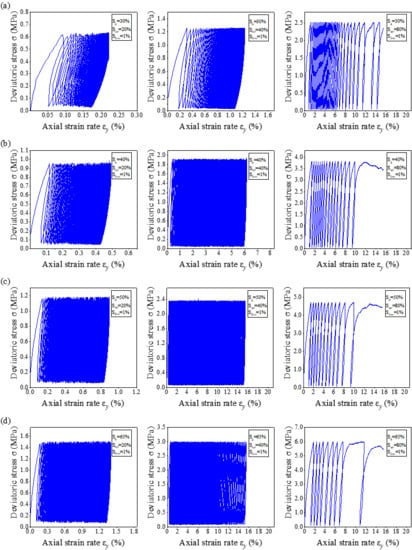
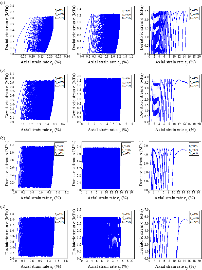
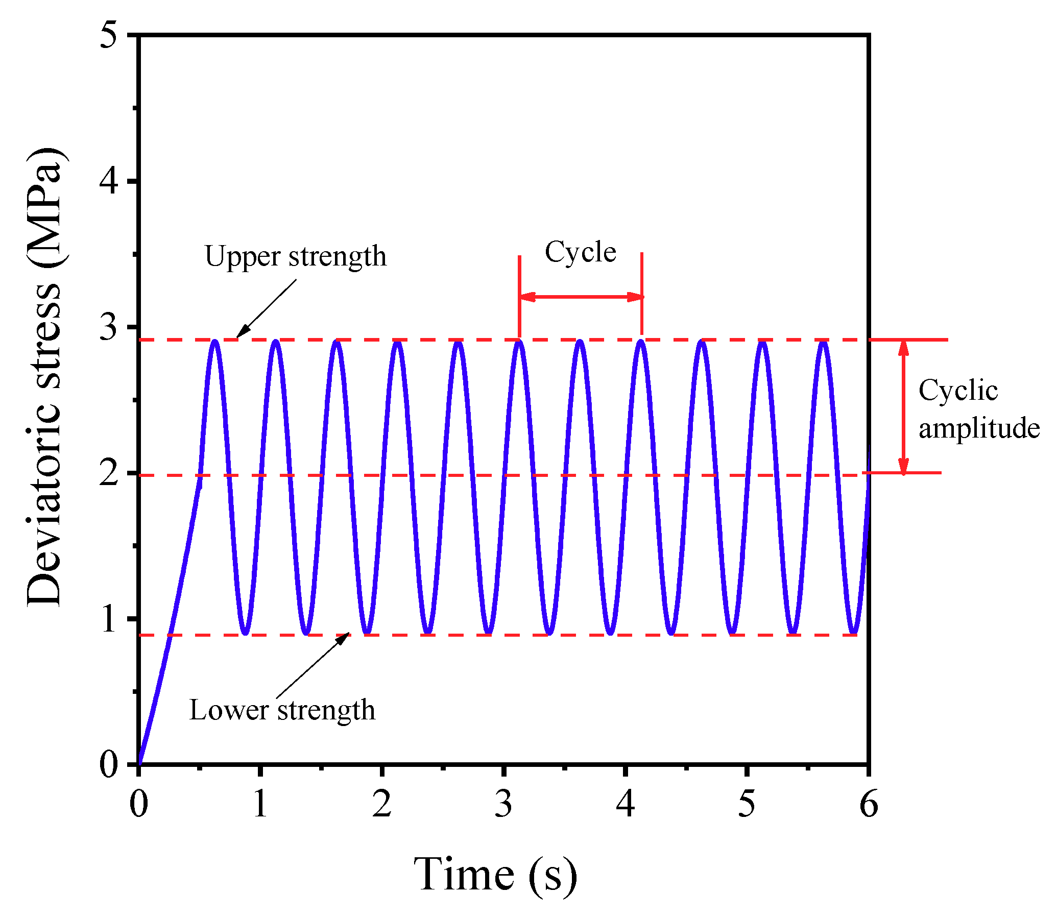
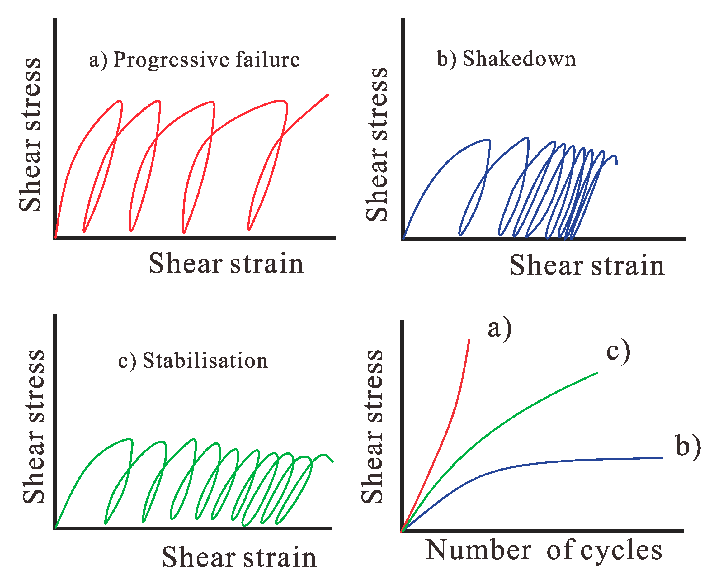
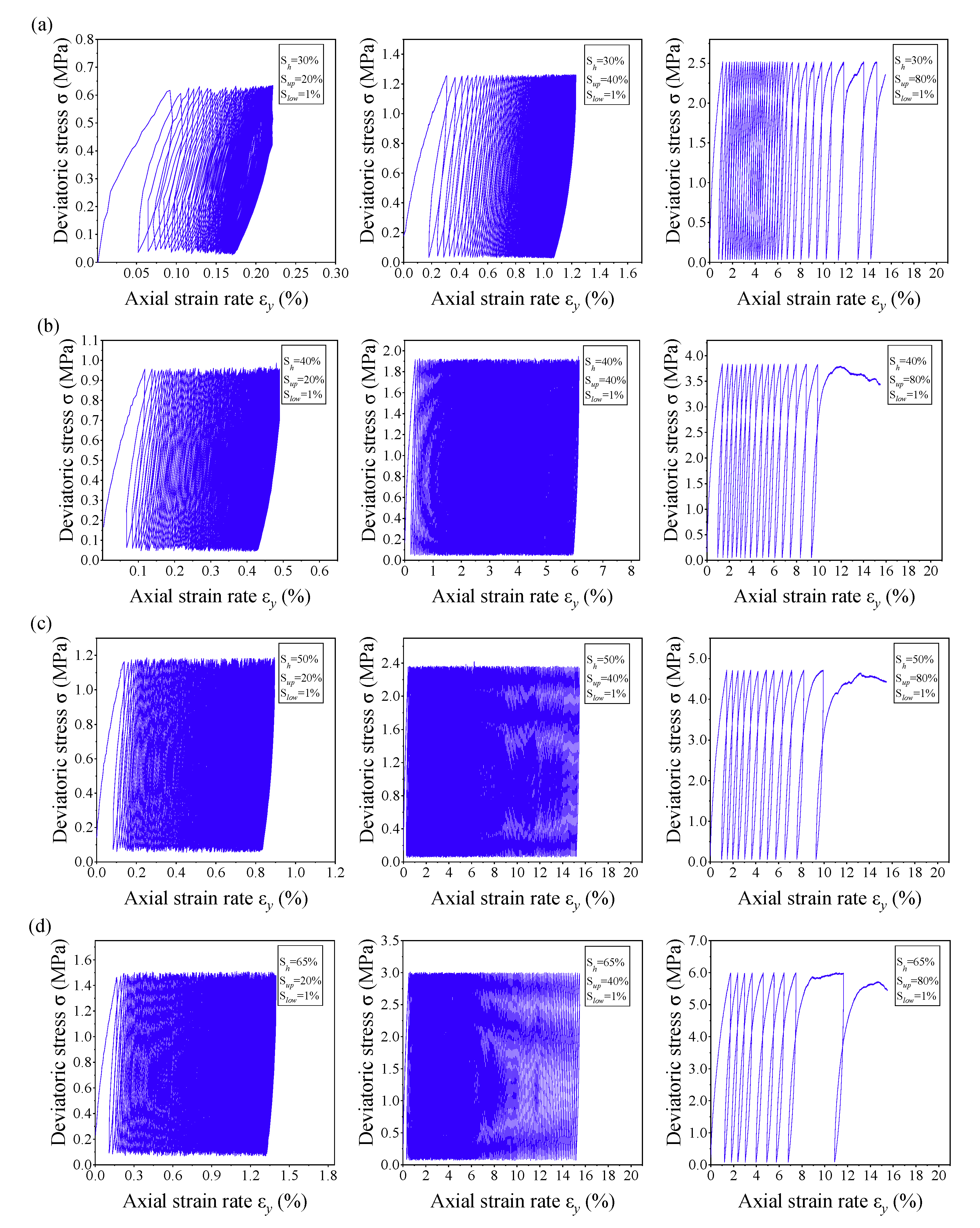
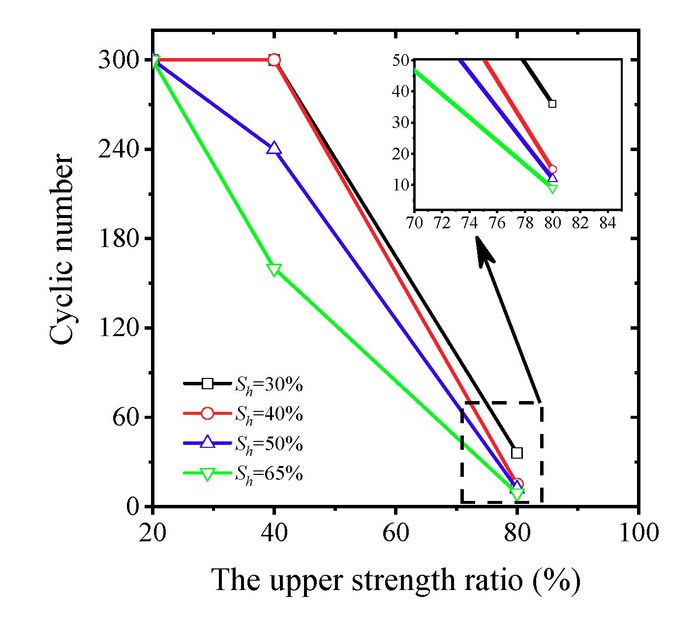
3.1.1. The Relationship between Dynamic Stress and Strain

According to the suggestion of Shajarati et al. [46], there are three main failure modes of soil under cyclic loading conditions. The main failure modes are progressive failure, stabilization, and shakedown, as shown in Figure 8. The models of the progessive failure and stabilization modes show that the soil specimens will reach failure in the two failure modes. In the progressive failure mode, the strain increment increases with the increasing number of cycles, while the strain increment decreases in the stabilization mode. In the shakedown mode, the strain increment decreases until the shear strain reaches a stable value, and the soil specimen will not reach failure.
Figure 9 shows the relationship between the deviatoric stress and the axial strain rate of MHS with different levels of hydrate saturation under various stress amplitude conditions. When the axial strain rate is more than 15%, the MHS can be considered to be damaged. As shown in Figure 9a, the hydrate saturation was 30%, and the peak strength was 3.16 MPa under monotonic loading conditions. The dynamic stress amplitudes were 0.6, 1.23, and 2.5 MPa, respectively. When the dynamic stress amplitude was 0.6 MPa, the axial strain rate was about 0.2% after 300 loading cycles. The axial strain rate was about 1.2% under a dynamic stress amplitude of 1.23 MPa. The axial strain rate increased as the hydrate saturation increased under the same upper strength ratio and the same loading cycle number. When Sh was 40% (see Figure 9 b), the final axial strain rates were 0.4% and 6.5% after 300 load–unload cycles when the dynamic stress amplitudes were 0.95 and 1.92 MPa, respectively. The hysteretic loop became less and less obvious, as the Sh increased when the upper strength ratio was less than 40%. When Sh values were equal to 50% and 65% and Sup was equal to 40%, as shown in Figure 9c,d, the specimens were damaged when the cycle number was less than 300. Moreover, when Sup was 80%, the specimens were more easily damaged as the hydrate saturation increased.
In this work, owing to the computational limitations, the biggest load–unload cyclic number was set to 300. Figure 10 shows the relationship between the cyclic number and the dynamic stress amplitude. The cyclic number decreased as the dynamic stress amplitude increased. The cyclic number decreased as the hydrate saturation increased. When the hydrate saturation was small, the rolling friction and sliding friction mainly controlled the shear strength of MHS. The specimens were not damaged unless the shear force was more than the friction force among particles and the cementation force of hydrate particles. As the hydrate content increased, the cementation force of the hydrates exceeded the shear stress of MHS. Plastic deformation developed gradually once the bonds among hydrates began to be destroyed. Thus, the specimens with higher hydrate saturations were damaged under fewer load–unload cycle numbers.

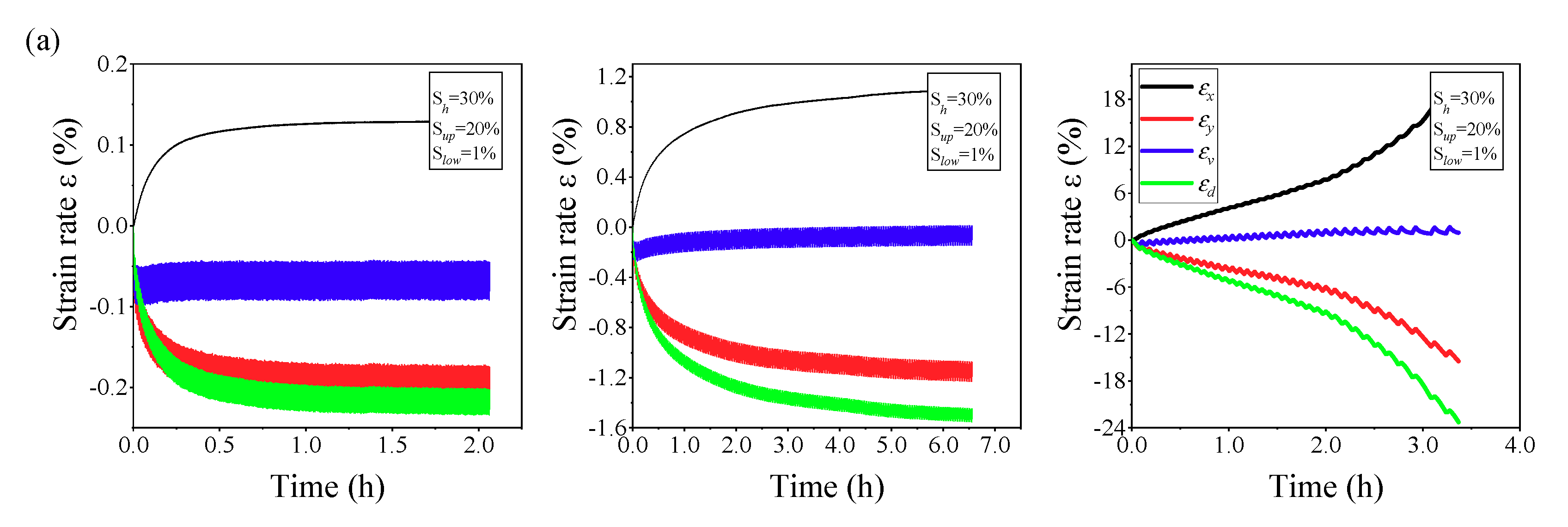
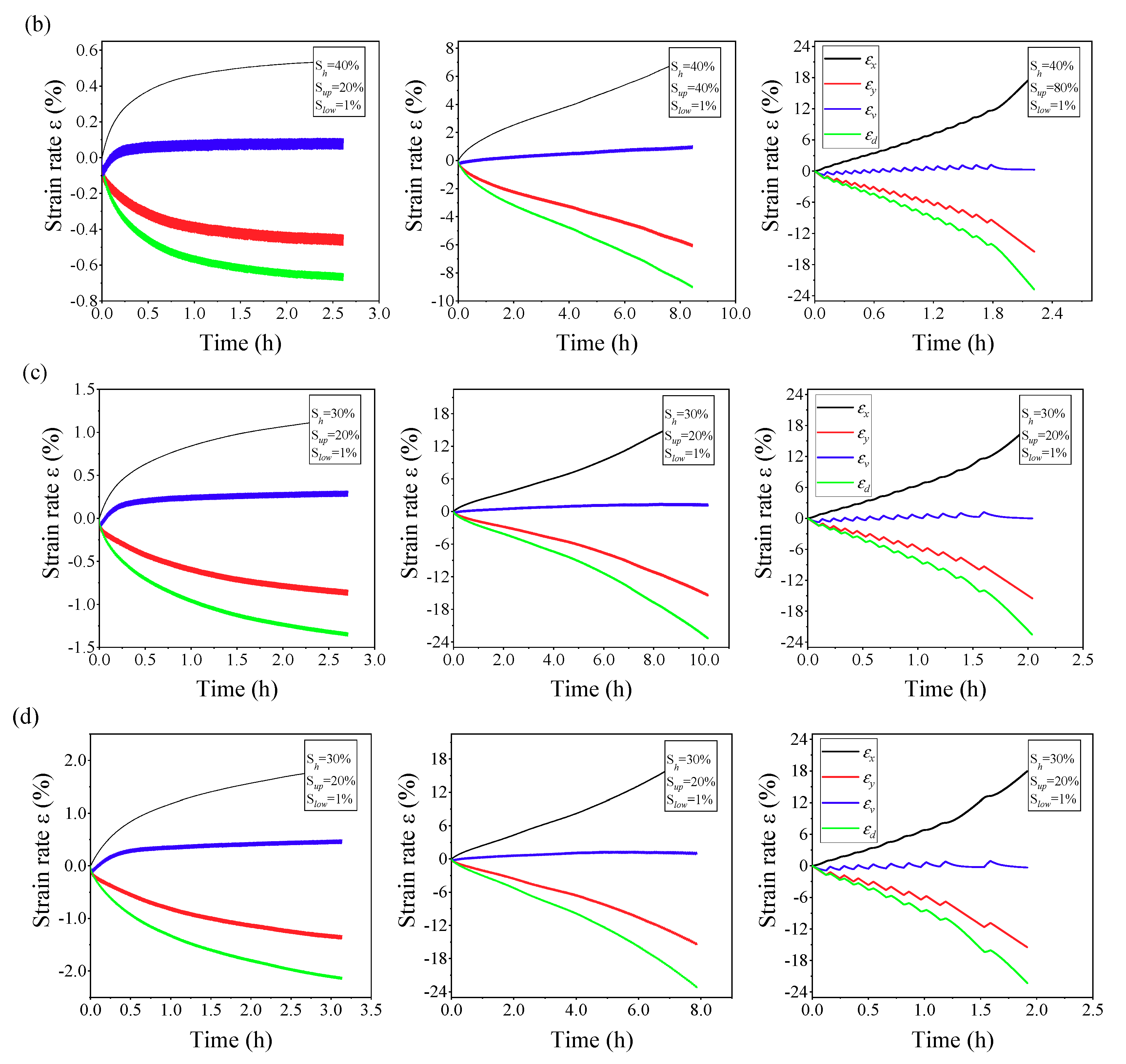
3.1.2. The Relationship of Strain versus Cyclic Time

In the present work, the volumetric strain εv is defined as dv/v0, where dv is the change of the specimen in volume and v0 is its initial volume before MHS shearing. In the biaxial simulation process, εv = εx + εy, where εx and εy are the lateral strain and vertical strain, respectively. The deviatoric strain εd is defined as εyεx.
Figure 11 shows the effects of the hydrate saturations and dynamic stress amplitudes on the evolutions of deviatoric strain, volumetric strain, and lateral strain. It shows that a larger dynamic stress amplitude led to a larger strain and less contractive behavior. By comparing Figure 11 with the main features of the failure modes (Figure 8), it is clear that the failure modes for the cases depended on the hydrate saturations and dynamic stress. When Sh = 30%, the failure mode was the shakedown mode, if the upper strength ratio was less than 40%, while the failure mode was the stabilization mode if the upper strength ratio increased to 80%. The failure mode changed as the hydrate saturation increased. The shakedown mode was present when Sh = 40% and Sup = 20%, while the failure mode changed to the progressive failure mode when the Sup = 40% or 80%, as shown in Figure 11b. In the cases where the Sh was 50% or 65%, the failure mode was the stabilization mode when Sup = 20%, while the failure mode developed into the progressive failure mode when Sup > 40%.
The specimen was relatively loose when the hydrate saturation was low. The particles were occlusal with each other after the specimen was compressed densely, and the force was transferred mainly by the soil particle skeleton under small dynamic amplitude conditions. The hydrate cementation was damaged when larger dynamic stress amplitude was present. The main movement pattern of particles was changed to slide, and the progressive failure mode dominated the failure process of MHS.

3.2. Micro-Mechanical Results

The microstructure of soils can be described by the coordination number and the arrangement of particles, contacts, etc. This work focused on the coordination number and the distribution of contacts and forces acting among particles.

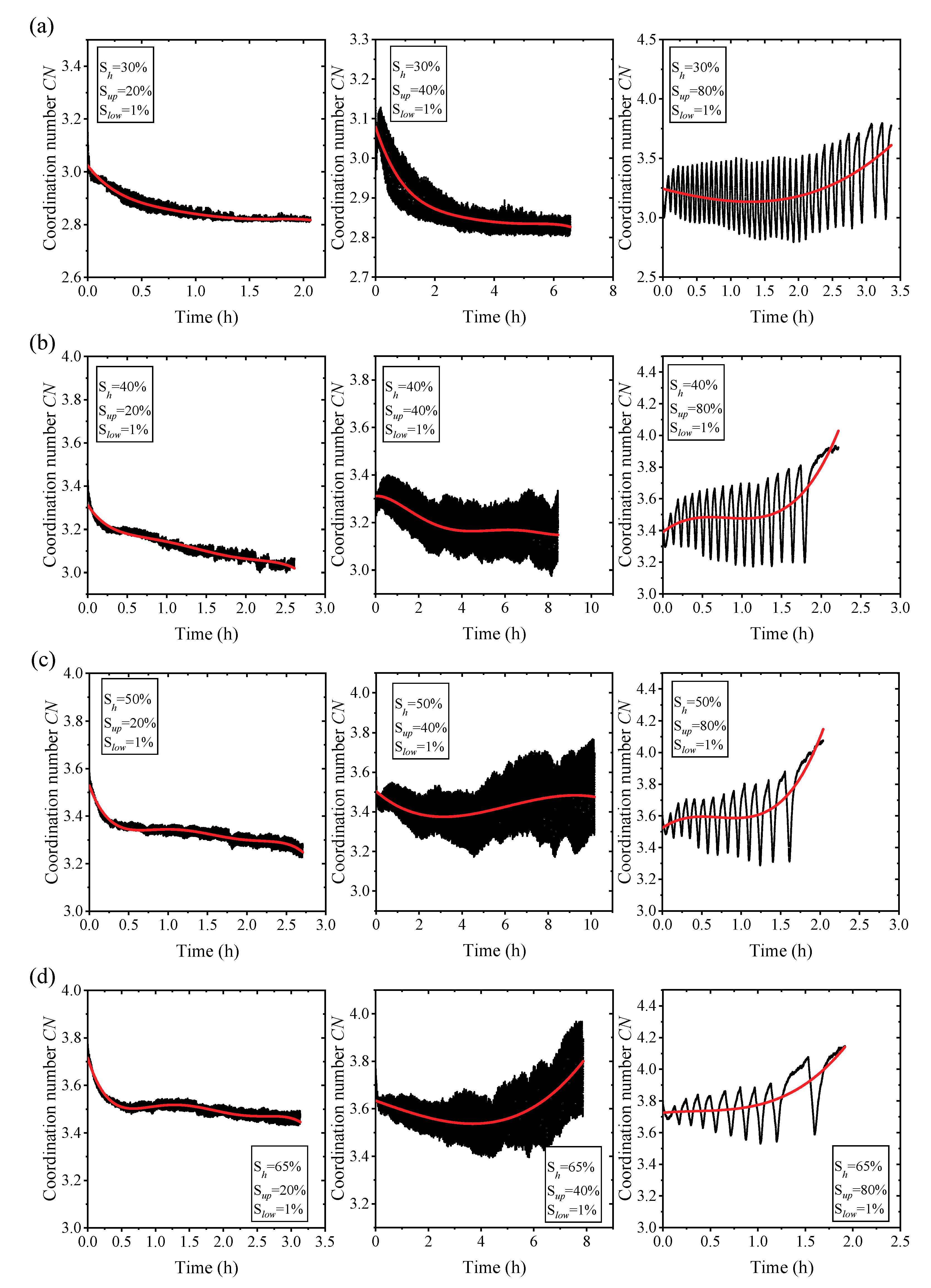
3.2.1. Coordination Number Evolution

The coordination number describes the average number of contacts per particle. The microstructures of soil specimens can be represented quantitatively throughout the whole shear processing of specimens. Figure 12 exhibits the evolution of the coordination number in MHS containing different hydrate contents under various dynamic stress amplitude conditions.
The MHS with various hydrate saturations showed similar trends: the coordination number reduced rapidly during the early stage of shearing and then approached a stable value when Sup = 20%. The initial coordination number increased from 3.1 to 3.8 as the hydrate saturation increased from 30% to 65%. However, in the upper strength level of the 40% condition, the variation in the coordination number between MHS with different levels of hydrate saturation was significantly different. The coordination number showed more and more fluctuations as the hydrate saturation increased, when Sup = 40%. This cumulative increase in the coordination number corresponded to the accumulation of compressive volumetric strain, as shown in Figure 11. The evolution of the coordination number was different for different failure modes. The fluctuation in the coordination number became more and more evident as the hydrate saturation increased from 30% to 65%, and the failure mode correspondingly changed from shakedown mode to progressive failure mode. This cumulative decrease in the coordination number corresponded to the dilatency of volumetric strain, as shown in Figure 11.

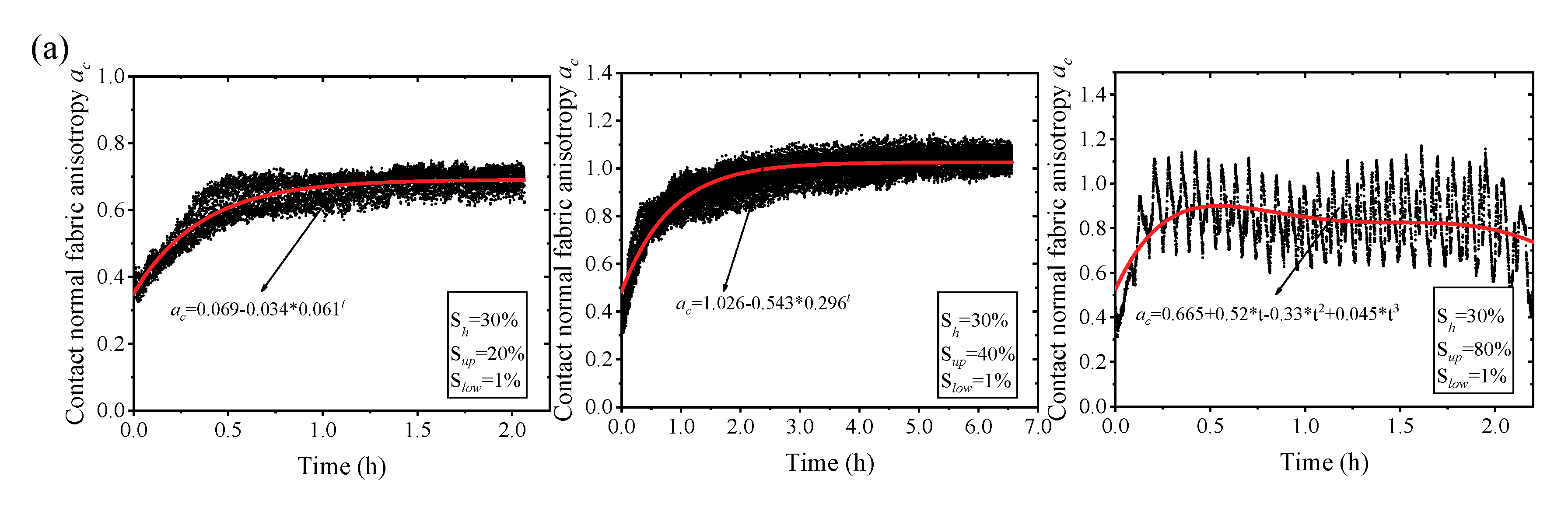
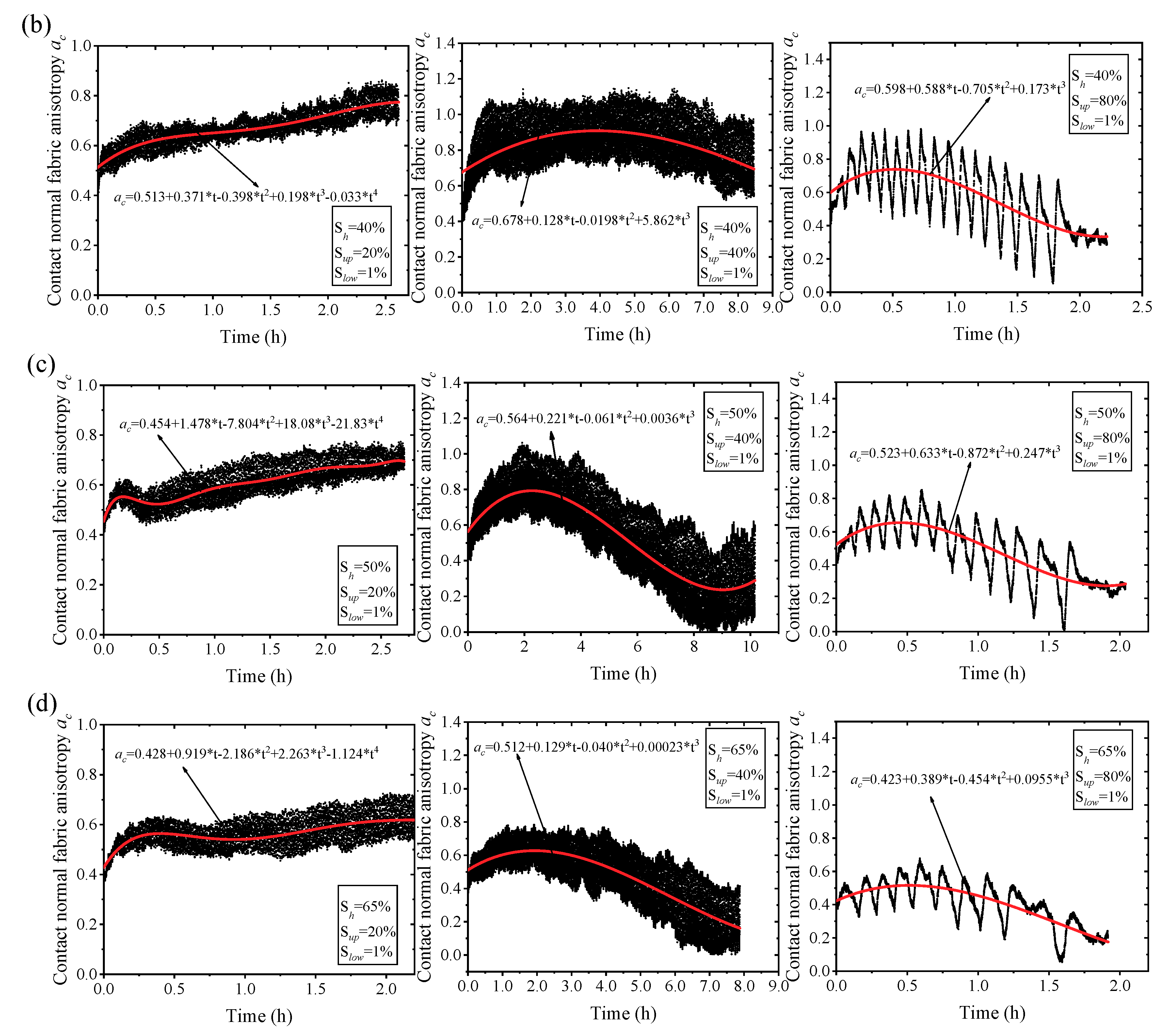
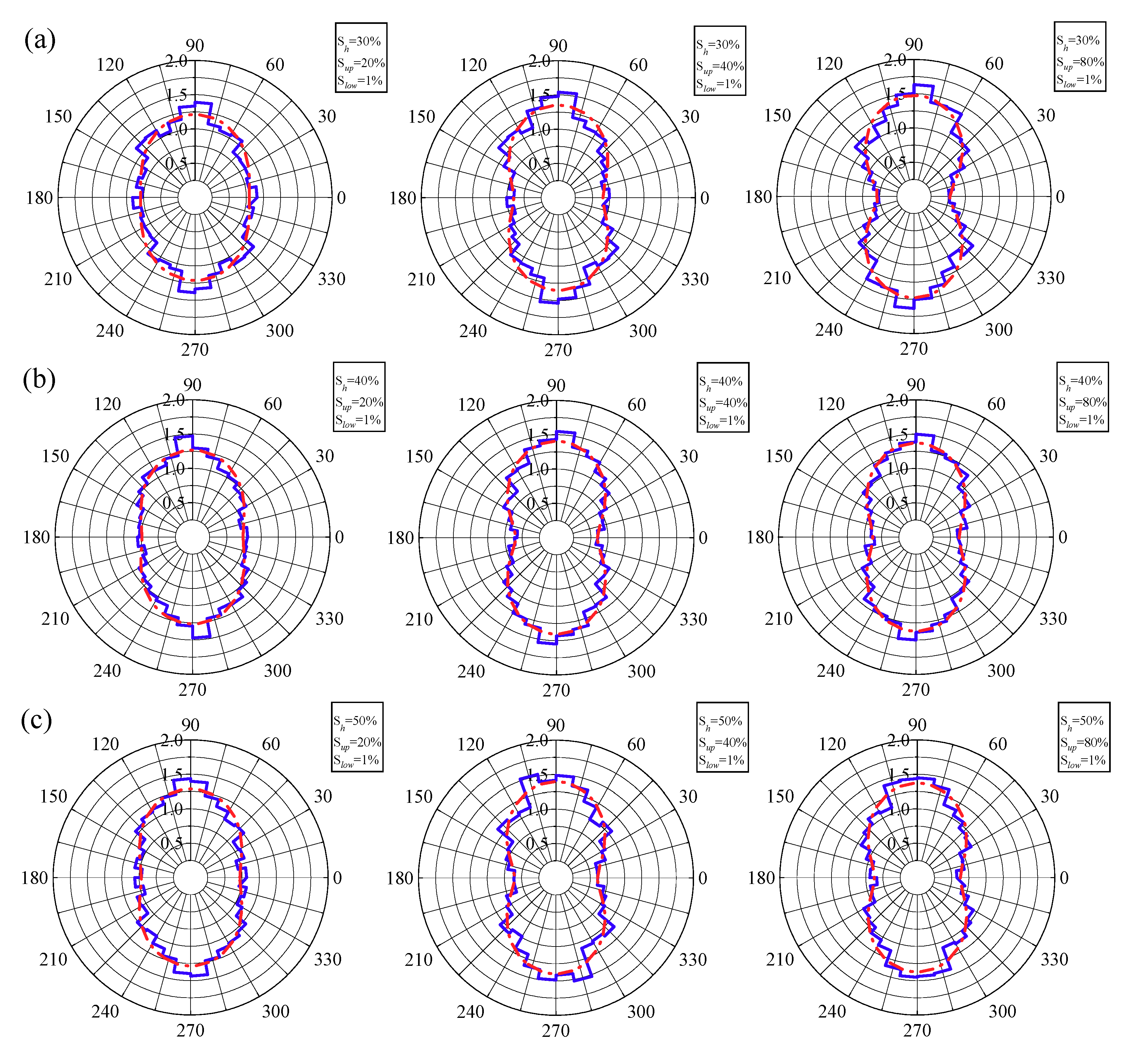
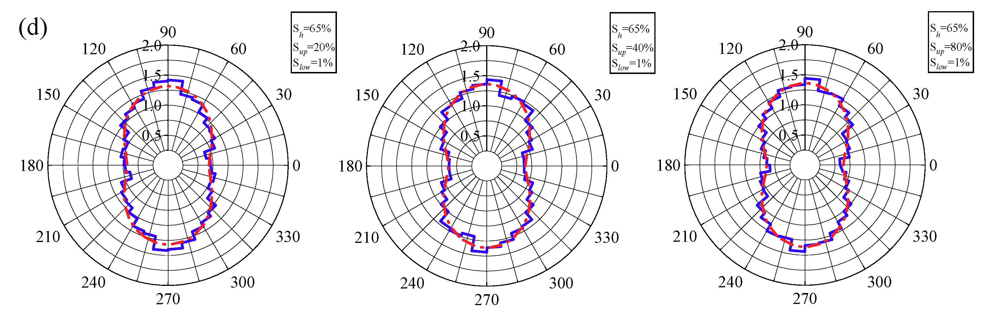
3.2.2. Contact Normal Fabric Evolution

In previous research, various fabric evolution approaches to constitutive modeling have been proposed for granular soils under cyclic loading, which can be divided into strain methods and stress methods. The fabric evolution can be evoluted by a plastic strain function [47]. In the following section, the fabric evolution of specimens under strain increments is calculated under cyclic loading conditions. Satake [48] and Oda [49] proposed a second-order fabric tensor to quantify the contact normal distribution between particles, and the fabric tensor was defined as follows:
F i j = Ω E ( Ω ) n i n j d Ω
where ni is the contact normal unit in the i-direction, and E ( Ω ) is the distribution probability function of the unit sphere Ω, expressed by a second-order Fourier expansion:
E ( Ω ) = 1 4 π [ 1 + a i j c n i n j ]
where a i j c is the second-order anisotropic tensor and can be derived from Equation (1) as follows:
a i j c = 15 2 R i j = 15 2 ( F i j 1 3 δ i j )
where Rij is the deviatoric part of the fabric tensor Fij and δ i j is the Kronecker delta.
To quantify the degree of fabric anisotropy, a scalar parameter ac was used as follows:
a c = a 11 c a 33 c
The evolution of ac with time is illustrated in Figure 13. The fabric anisotropy of specimens showed different characteristics during the loading and unloading processes. The contact was disrupted in the horizontal direction while more contacts formed in the vertical direction, and the fabric anisotropy reached the highest value at the end of loading. During unloading, the value of ac gradually decreased. This means that the fabric was anisotropic with the contact normal concentrating in the vertical direction, though the stress was in an isotropic state. This result is similar to the result of O’Sullivan and Cui [50]. When Sh = 30%, the value of ac first increased as the simulating time increased and then fluctuated around a stable value. When Sh = 40%, 50%, or 60%, the value of ac gradually increased as the simulating time increased under the condition of Sup = 20%, while the value of ac first increased, and then, decreased as the simulating time increased, when Sup = 40% or 80%. Thus, there may be a threshold value for the fabric anisotropy under cyclic loading. The fabric structure of the test specimen will change to unstable if the threshold is reached. During cyclic loading, the test specimens remain stable, and the fabric evolution between the cyclic loading condition and the monotonic loading conditon is much more complicated.

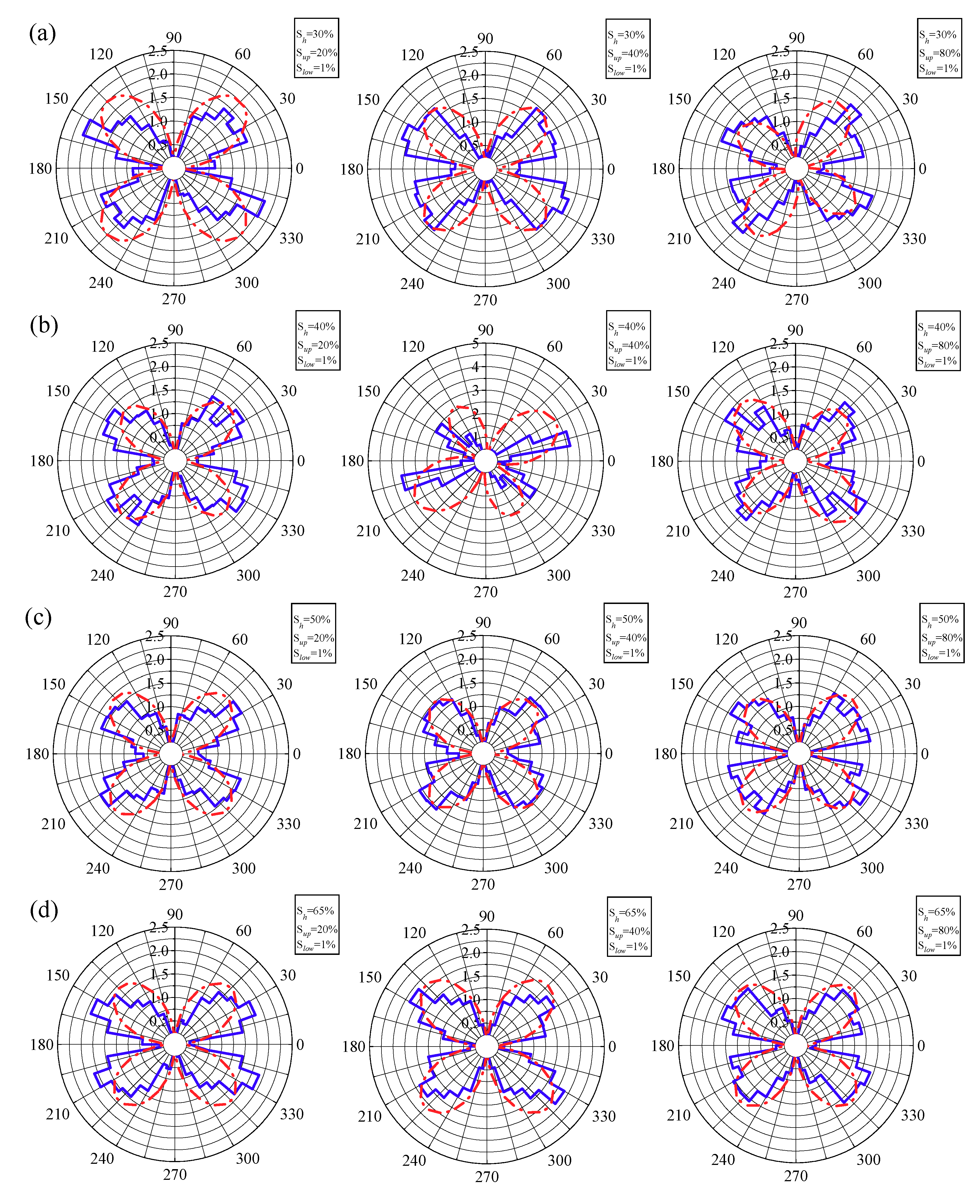
3.2.3. Stress–Force–Fabric Relationship

The geometrical anisotropy which describes the distribution of the contact normal orientations is commonly described using the fabric anisotropy. The mechanical anisotropy that describes the distribution of the contact force’s direction is also anisotropic [51]. The mechanical anisotropy can be split into normal force anisotropy and tangential force anisotropy. The fabric tensors of the contact force in the normal direction and tangential direction can be respectively defined as follows:
σ i j = N C V 0 2 π f i ¯ ( θ ) l j ¯ ( θ ) E ( θ ) d θ = N C V 0 2 π ( f n ¯ ( θ ) n i + f t ¯ ( θ ) t i ) l n ¯ ( θ ) n i E ( θ ) d θ
where E ( θ ) represents the probability density function of the contact orientation for any angle θ; f n ¯ ( θ ) and   f t ¯ ( θ ) respectively represent the average normal and tangential force; l n ¯ ( θ ) is the average length of branch vectors. The second-order Fourier series expressions can be described in a polar coordinate system. The probability density functions are the following:
E ( θ ) = 1 2 π [ 1 + a c cos 2 ( θ θ c ) ]
f n ¯ ( θ ) = f 0 ¯ [ 1 + a n cos 2 ( θ θ f n ) ]
f t ¯ ( θ ) = f 0 ¯ a t cos 2 ( θ θ f t )
l n ¯ ( θ ) = l 0 ¯ [ 1 + a l cos 2 ( θ θ l ) ]
where ac, an, at, and al represent the anisotropy coefficient of the contact normal, the magnitude coefficient of the normal contact force, the magnitude coefficient of the tangential contact force, and the magnitude of anisotropy for the branch vector; the angles θc, θfn, θft, and θl represent the corresponding privileged directions following the principal stress direction in a sheared state; f0 is the average normal contact force for different values of θ; and l0 is the average length of the normal contact vector when θf0 and l0 are different from the average normal force and the average length of the normal contact vector’s overall contact [52].
Figure 14 presents the distribution of the normal contact force of the MHS under various dynamic stress amplitudes conditions. When Sup = 20%, the anisotropic was not evident, and the distribution of the normal contact force was in an elliptical shape. As the upper strength ratio increased, the distribution of normal contact force changed to a “peanut shape.” In all cases, the main direction of the normal contact force was consistent with the loading direction (θfn = 90°). Figure 15 presents the distribution of the shear contact force of the MHS. The distribution of the shear contact force under cyclic loading shear tests was evenly distributed in the directions of 45°, 135°, 225°, and 315° as a “flower shape”. The MHS consist of soil particles and hydrate particles, and hydrate particles mainly bond to soil particles. Therefore, the normal contact force mainly transfers through the soil particle’s skeleton.

4. Conclusions

The main purpose of the present work was to obtain a better understanding of the microstructural evolution of MHS under cyclic loading conditions and to aid in the development of micromechanical-based constitutive models. To achieve this aim, a series of drained, cyclic biaxial compressive tests under constant stress amplitudes were numerically carried out with the DEM, and the cementing of hydrate particles and the rolling resistance among particles were considered.
The cyclic loading number decreased as the hydrate saturation increased, when the MHS were damaged. The failure mode of the MHS was found to depend on the dynamic stress amplitude and the hydrate saturation. The microstructures of the MHS during the cyclic loading shear process were also analyzed. When Sh = 30%, the value of ac first increased as the simulation time increased, and then fluctuated around a stable value. When Sh = 40%, 50%, and 60%, the value of ac gradually increased as the simulation time increased under the condition of Sup = 20%, while the value of ac first increased and then decreased as the simulation time increased, when Sup = 40% and 80%. Therefore, it seems that a threshold value exists for the fabric anisotropy under cyclic loading, and once the threshold is reached, the fabric structure of the specimen tends to be unstable. In all cases, the main direction of the normal contact force was consistent with the loading direction. The MHS consists of soil particles and hydrate particles, and hydrate particles mainly bond to soil particles. Therefore, the normal contact force mainly transfers through the soil particle skeleton.

Author Contributions

Y.J. conceived the presented idea. B.G. designed the model and the computational framework, and wrote the manuscript. D.W. analyzed the data. B.G. verified the analytical data.

Funding

This study was partially funded by the National Natural Science Foundation of China (grant number 51804180); the China Scholarship Council (CSC number 201608370083); the Key Research and Development Plan of Shandong Province (grant number 2018GSF116007); the Open Project of the State Key Laboratory for Geomechanics and Deep Underground Engineering in CUMTB (number SKLGDUEK1727); the Open Project of the State Key Laboratory of Mining Disaster Prevention and Control, Co-founded by Shandong Province; and the Ministry of Science and Technology (number MDPC201609). Their support is gratefully acknowledged.

Conflicts of Interest

The authors declare no conflicts of interest.

References

  1. Makogon, Y.; Omelchenko, R.Y. Engineering. Commercial gas production from Messoyakha deposit in hydrate conditions. J. Nat. Gas Sci. Eng. 2013, 11, 1–6. [Google Scholar] [CrossRef]
  2. Kurihara, M.; Funatsu, K.; Ouchi, H.; Masuda, Y.; Yamamoto, K.; Narita, H.; Dallimore, S.R.; Collett, T.S.; Hancock, S.H. Analyses of production tests and MDT tests conducted in Mallik and Alaska methane hydrate reservoirs: What can we learn from these well tests? In Proceedings of the the 6th International Conference of Gas Hydrates, Vancouver, BC, Canada, 6–10 July 2008. [Google Scholar]
  3. Fujii, T.; Suzuki, K.; Takayama, T.; Tamaki, M.; Komatsu, Y.; Konno, Y.; Yoneda, J.; Yamamoto, K.; Nagao, J.J.M.; Geology, P. Geological setting and characterization of a methane hydrate reservoir distributed at the first offshore production test site on the Daini-Atsumi Knoll in the eastern Nankai Trough, Japan. Mar. Pet. Geol. 2015, 66, 310–322. [Google Scholar] [CrossRef]
  4. Tanigawa, K.; Shishikura, M.; Fujiwara, O.; Namegaya, Y.; Matsumoto, D.J.T.H. Mid-to late-Holocene marine inundations inferred from coastal deposits facing the Nankai Trough in Nankoku, Kochi Prefecture, southern Japan. Holocene 2018, 28, 867–878. [Google Scholar] [CrossRef]
  5. Li, J.-f.; Ye, J.-l.; Qin, X.-w.; Qiu, H.-j.; Wu, N.-y.; Lu, H.-l.; Xie, W.-w.; Lu, J.-a.; Peng, F.; Xu, Z.-q.J.C.G. The first offshore natural gas hydrate production test in South China Sea. China Geol. 2018, 1, 5–16. [Google Scholar] [CrossRef]
  6. Shouwei, Z.; Qingping, L.; Wei, C.; Jianliang, Z.; Weixin, P.; Yufa, H.; Xin, L.; Liangbin, X.; Qiang, F.; Jiang, L. The World’s First Successful Implementation of Solid Fluidization Well Testing and Production for Non-Diagenetic Natural Gas Hydrate Buried in Shallow Layer in Deep Water. In Proceedings of the Offshore Technology Conference, Houston, TX, USA, 30 April–3 May 2018. [Google Scholar]
  7. Winters, W.J.; Waite, W.F.; Mason, D.; Gilbert, L.; Pecher, I. Methane gas hydrate effect on sediment acoustic and strength properties. J. Pet. Sci. Eng. 2007, 56, 127–135. [Google Scholar] [CrossRef]
  8. Priest, J.A.; Druce, M.; Roberts, J.; Schultheiss, P.; Nakatsuka, Y.; Suzuki, K. PCATS Triaxial: A new geotechnical apparatus for characterizing pressure cores from the Nankai Trough, Japan. Mar. Pet. Geol. 2015, 66, 460–470. [Google Scholar] [CrossRef]
  9. Yoneda, J.; Masui, A.; Konno, Y.; Jin, Y.; Egawa, K.; Kida, M.; Ito, T.; Nagao, J.; Tenma, N. Mechanical properties of hydrate-bearing turbidite reservoir in the first gas production test site of the Eastern Nankai Trough. Mar. Pet. Geol. 2015, 66, 471–486. [Google Scholar] [CrossRef]
  10. Yoneda, J.; Masui, A.; Konno, Y.; Jin, Y.; Kida, M.; Katagiri, J.; Nagao, J.; Tenma, N. Pressure-core-based reservoir characterization for geomechanics: Insights from gas hydrate drilling during 2012–2013 at the eastern Nankai Trough. Mar. Pet. Geol. 2017, 86, 1–16. [Google Scholar] [CrossRef]
  11. Priest, J.A.; Clayton, C.R.; Rees, E.V. Potential impact of gas hydrate and its dissociation on the strength of host sediment in the Krishna–Godavari Basin. Mar. Pet. Geol. 2014, 58, 187–198. [Google Scholar] [CrossRef]
  12. Masui, A.; Haneda, H.; Ogata, Y.; Aoki, K. The effect of saturation degree of methane hydrate on the shear strength of synthetic methane hydrate sediments. In Proceedings of the 5th International Conference on Gas Hydrates, Trondheim, Norway, 13–16 June 2005; pp. 657–663. [Google Scholar]
  13. Miyazaki, K.; Masui, A.; Sakamoto, Y.; Tenma, N.; Yamaguchi, T. Effect of confining pressure on triaxial compressive properties of artificial methane hydrate bearing sediments. In Proceedings of the Offshore Technology Conference, Houston, TX, USA, 3–6 May 2010. [Google Scholar]
  14. Miyazaki, K.; Masui, A.; Tenma, N.; Ogata, Y.; Aoki, K.; Yamaguchi, T.; Sakamoto, Y. Study on mechanical behavior for methane hydrate sediment based on constant strain-rate test and unloading-reloading test under triaxial compression. Int. J. Offshore Polar Eng. 2010, 20, 61–67. [Google Scholar]
  15. Hyodo, M.; Li, Y.; Yoneda, J.; Nakata, Y.; Yoshimoto, N.; Kajiyama, S.; Nishimura, A.; Song, Y. A comparative analysis of the mechanical behavior of carbon dioxide and methane hydrate-bearing sediments. Am. Mineral. 2014, 99, 178–183. [Google Scholar] [CrossRef]
  16. Hyodo, M.; Li, Y.; Yoneda, J.; Nakata, Y.; Yoshimoto, N.; Nishimura, A. Effects of dissociation on the shear strength and deformation behavior of methane hydrate-bearing sediments. Mar. Pet. Geol. 2014, 51, 52–62. [Google Scholar] [CrossRef]
  17. Hyodo, M.; Li, Y.; Yoneda, J.; Nakata, Y.; Yoshimoto, N.; Nishimura, A.; Song, Y. Mechanical behavior of gas strength and deformation behavior of methane. J. Geophys. Res. Solid Earth 2013, 118, 5185–5194. [Google Scholar] [CrossRef]
  18. Hyodo, M.; Nakata, Y.; Yoshimoto, N.; Yoneda, J. Shear strength of methane hydrate bearing sand and its deformation during dissociation of methane hydrate. In Proceedings of the 4th International Symposium on Deformation Characteristics of Geomaterials, Atlanta, GA, USA, 15 September 2008; pp. 549–556. [Google Scholar]
  19. Hyodo, M.; Yoneda, J.; Yoshimoto, N.; Nakata, Y. Mechanical and dissociation properties of methane hydrate-bearing sand in deep seabed. Soils Found. 2013, 53, 299–314. [Google Scholar] [CrossRef] [Green Version]
  20. Miyazaki, K.; Masui, A.; Sakamoto, Y.; Aoki, K.; Tenma, N.; Yamaguchi, T. Triaxial compressive properties of artificial methane-hydrate-bearing sediment. J. Geophys. Res. Solid Earth 2011, 116, 1–11. [Google Scholar] [CrossRef]
  21. Li, Y.; Song, Y.; Liu, W.; Yu, F.; Wang, R.; Nie, X. Analysis of mechanical properties and strength criteria of methane hydrate-bearing sediments. Int. J. Offshore Polar Eng. 2012, 22, 290–296. [Google Scholar]
  22. Liu, Z.; Wei, H.; Peng, L.; Wei, C.; Ning, F. An easy and efficient way to evaluate mechanical properties of gas hydrate-bearing sediments: The direct shear test. J. Pet. Sci. Eng. 2017, 149, 56–64. [Google Scholar] [CrossRef]
  23. Kajiyama, S.; Wu, Y.; Hyodo, M.; Nakata, Y.; Nakashima, K.; Yoshimoto, N. Experimental investigation on the mechanical properties of methane hydrate-bearing sand formed with rounded particles. J. Nat. Gas Sci. Eng. 2017, 45, 96–107. [Google Scholar] [CrossRef]
  24. Kajiyama, S.; Nishimura, A.; Hyodo, M. Shear Behaviour and Localized Deformation of Methane Hydrate-Bearing Sand using High Pressure Plane Strain Shear Tests. In Proceedings of the Eleventh Ocean Mining and Gas Hydrates Symposium, Kona, HI, USA, 21–27 June 2015. [Google Scholar]
  25. Gong, B.; Jiang, Y.; Chen, L.J. Feasibility investigation of the mechanical behavior of methane hydrate-bearing specimens using the multiple failure method. J. Nat. Gas Sci. Eng. 2019, 69, 102915. [Google Scholar] [CrossRef]
  26. Mienert, J.; Vanneste, M.; Bünz, S.; Andreassen, K.; Haflidason, H.; Sejrup, H.P.J.M.; Geology, P. Ocean warming and gas hydrate stability on the mid-Norwegian margin at the Storegga Slide. Mar. Pet. Geol. 2005, 22, 233–244. [Google Scholar] [CrossRef]
  27. Sultan, N.; Cochonat, P.; Foucher, J.-P.; Mienert, J. Effect of gas hydrates melting on seafloor slope instability. Mar. Geol. 2004, 213, 379–401. [Google Scholar] [CrossRef] [Green Version]
  28. Wright, S.; Rathje, E.M.J.P.; Geophysics, A. Triggering mechanisms of slope instability and their relationship to earthquakes and tsunamis. Pure Appl. Geophys. 2003, 160, 1865–1877. [Google Scholar] [CrossRef]
  29. Tappin, D.R.; Matsumoto, T.; Watts, P.; Satake, K.; McMurtry, G.M.; Matsuyama, M.; Lafoy, Y.; Tsuji, Y.; Kanamatsu, T.; Lus, W.J.E.; et al. Sediment slump likely caused 1998 Papua New Guinea tsunami. Eos Trans. Am. Geophys. Un. 1999, 80, 329–340. [Google Scholar] [CrossRef]
  30. Kawata, Y.; Benson, B.C.; Borrero, J.C.; Borrero, J.L.; Davies, H.L.; de Lange, W.P.; Imamura, F.; Letz, H.; Nott, J.; Synolakis, C.E.J.E.; et al. Tsunami in Papua New Guinea was as intense as first thought. Eos Trans. Am. Geophys. Un. 1999, 80, 101–105. [Google Scholar] [CrossRef]
  31. Erdik, M. Report on 1999 Kocaeli and Düzce (Turkey) Earthquakes; Boğaziçi Üniversitesi, Kandilli Rasathanesi ve Deprem Araştirma Enstitüsü: Istanbul, Turkey, 2000. [Google Scholar]
  32. Clayton, C.; Priest, J.; Best, A.J.G. The effects of disseminated methane hydrate on the dynamic stiffness and damping of a sand. Geotechnique 2005, 55, 423–434. [Google Scholar] [CrossRef]
  33. Priest, J.A.; Best, A.I.; Clayton, C.R. Attenuation of seismic waves in methane gas hydrate-bearing sand. Geophys. J. Int. 2006, 164, 149–159. [Google Scholar] [CrossRef] [Green Version]
  34. Kingston, E.; Clayton, C.; Priest, J.; Best, A. Effect of grain characteristics on the behaviour of disseminated methane hydrate bearing sediments. In Proceedings of the 6th International Conference on Gas Hydrates (ICGH 2008), Vancouver, BC, Canada, 6–10 July 2008. [Google Scholar]
  35. Lee, J.; Francisca, F.M.; Santamarina, J.C.; Ruppel, C. Parametric study of the physical properties of hydrateed methansand, silt, and clay sediments: 2. Small-strain mechanical properties. J. Geophys. Res. Solid Earth 2010, 115, 1–11. [Google Scholar]
  36. Zhang, X.; Lu, X.; Wang, S.; Li, Q.J.R.S.M. Experimental study of static and dynamic properties of tetrahydrofuran hydrate-bearing sediments. Rock Soil Mech. 2011, 32, 303–308. [Google Scholar]
  37. Cundall, P.A.; Strack, O.D.J.g. A discrete numerical model for granular assemblies. Geotechnique 1979, 29, 47–65. [Google Scholar] [CrossRef]
  38. Cho, N.a.; Martin, C.; Sego, D.J.I.J.o.R.M.; Sciences, M. A clumped particle model for rock. Int. J. Rock Mech. Min. Sci. 2007, 44, 997–1010. [Google Scholar] [CrossRef]
  39. Castro-Filgueira, U.; Alejano, L.; Arzúa, J.; Ivars, D.M.J.P.e. Sensitivity analysis of the micro-parameters used in a PFC analysis towards the mechanical properties of rocks. Procedia Eng. 2017, 191, 488–495. [Google Scholar] [CrossRef]
  40. Cao, R.-h.; Cao, P.; Lin, H.; Pu, C.-z.; Ou, K.J.R.M.; Engineering, R. Mechanical behavior of brittle rock-like specimens with pre-existing fissures under uniaxial loading: Experimental studies and particle mechanics approach. Rock Mech. Rock Eng. 2016, 49, 763–783. [Google Scholar] [CrossRef]
  41. Yang, S.-Q.; Huang, Y.-H.; Jing, H.-W.; Liu, X.-R.J.E.G. Discrete element modeling on fracture coalescence behavior of red sandstone containing two unparallel fissures under uniaxial compression. Eng. Geol. 2014, 178, 28–48. [Google Scholar] [CrossRef]
  42. Jiang, Y.; Gong, B. Discrete-element numerical modelling method for studying mechanical response of methane-hydrate-bearing specimens. Mar. Georesources Geotechnol. 2019, 38, 1–15. [Google Scholar] [CrossRef]
  43. Masui, A.; Haneda, H.; Ogata, Y.; Aoki, K. Triaxial Compression test on submarine sediment containing methane hydrate in deep sea off the coast off Japan. In Proceedings of the 41st Annual Conference, Japanese Geotechnical Society, Tokyo, Japan, 9–13 November 2015. [Google Scholar]
  44. De Alba, P.; Chan, C.K.; Seed, H.B. Determination of Soil Liquefaction Characteristics by Large-Scale Laboratory Tests; Shannon & Wilson: Seattle, DC, USA, 1976; Volume 27. [Google Scholar]
  45. Seed, H.B.; Idriss, I.M.J.J.o.S.M.; Div, F. Simplified procedure for evaluating soil liquefaction potential. J. Soil Mech. Found. Division 1971, 97, 1249–1273. [Google Scholar]
  46. Jiang, M.; Zhang, A.; Li, T. Distinct element analysis of the microstructure evolution in granular soils under cyclic loading. Granul. Matter 2019, 21, 38–53. [Google Scholar] [CrossRef]
  47. Wan, R.G.; Guo, P.J.J.J.o.E.M. Stress dilatancy and fabric dependencies on sand behavior. J. Eng. Mech. 2004, 130, 635–645. [Google Scholar] [CrossRef]
  48. Satake, M. Fabric tensor in granular materials. In Proceedings of the IUTAM Conference on Deformation and Flow of Granular Materials, Delft, the Netherlands, 31 August–3 September 1982; pp. 63–68. [Google Scholar]
  49. Oda, M.J.S. Initial fabrics and their relations to mechanical properties of granular material. Soils Found. 1972, 12, 17–36. [Google Scholar] [CrossRef]
  50. O’Sullivan, C.; Cui, L.J.P.T. Micromechanics of granular material response during load reversals: Combined DEM and experimental study. Powder Technol. 2009, 193, 289–302. [Google Scholar] [CrossRef] [Green Version]
  51. Cambou, B.; Dubujet, P.; Nouguier-Lehon, C. Anisotropy in granular materials at different scales. Mech. Mater. 2004, 36, 1185–1194. [Google Scholar] [CrossRef]
  52. Gong, J.; Liu, J.J.C. Mechanical transitional behavior of binary mixtures via DEM: Effect of differences in contact-type friction coefficients. Comput. Geotech. 2017, 85, 1–14. [Google Scholar] [CrossRef]
Figure 1. High-resolution seismic reflection profile of Storegga Slide [26].
Energies 12 03694 g001
Figure 2. Cohesive model and its micromechanical behavior schematic diagram: (a) parallel bond model; (b) rolling resistance model [38].
Energies 12 03694 g002
Figure 3. The “trial and error” method used to check the process of the particle flow code (PFC) model (Modified from Castro-Filgueira et al. (2017) [39].
Energies 12 03694 g003
Figure 4. The particle size distribution of soil grains in the simulation and experimental test.
Energies 12 03694 g004
Figure 5. Distinct element method (DEM) simulation model of the methane hydrate-bearing specimen.
Energies 12 03694 g005
Figure 6. Stress–strain behaviors of methane hydrate-bearing sediments (MHS) with different hydrate saturation (Sh) levels in laboratory tests and the simulation [42].
Energies 12 03694 g006
Figure 7. Loading waveform schematic.
Energies 12 03694 g007
Figure 8. Failure modes of granular soils due to cyclic loading. Modified from Shajarati et al. (2012) [46].
Energies 12 03694 g008
Figure 9. Dynamic stress–strain curves for MHS under different dynamic stress amplitudes and various Sh conditions. (a) Sh = 30%; (b) Sh = 40%; (c) Sh = 50%; (d) Sh = 65%.
Energies 12 03694 g009
Figure 10. The relationship between the upper strength ratio and the cyclic number.
Energies 12 03694 g010
Figure 11. The effect of the dynamic stress amplitude on the strain of the MHS with different Sh values. (a) Sh = 30%; (b) Sh = 40%; (c) Sh = 50%; (d) Sh = 65%.
Energies 12 03694 g011aEnergies 12 03694 g011b
Figure 12. The evolution of the coordination number under different dynamic amplitude conditions for the MHS with different Sh values. (a) Sh = 30%; (b) Sh = 40%; (c) Sh = 50%; (d) Sh = 65%.
Energies 12 03694 g012
Figure 13. The evolution of contact normal fabric anisotropy under different dynamic amplitude conditions for MHS with different Sh values. (a) Sh = 30%; (b) Sh = 40%; (c) Sh = 50%; (d) Sh = 65%.
Energies 12 03694 g013aEnergies 12 03694 g013b
Figure 14. The evolution of the normal contact force between the particles under different dynamic amplitude conditions for MHS with different Sh values. (a) Sh = 30%; (b) Sh = 40%; (c) Sh = 50%; (d) Sh = 65%.
Energies 12 03694 g014aEnergies 12 03694 g014b
Figure 15. The evolution of the shear contact force between the particles under different dynamic amplitude conditions for the MHS with different Sh values. (a) Sh = 30%; (b) Sh = 40%; (c) Sh = 50%; (d) Sh = 65%.
Energies 12 03694 g015
Table 1. Mechanical parameters of particles in the simulation.
PropertySoilMethane Hydrate
Density (kg/m3)2500320
Particle sizes, D (mm)0.01–0.40.006
Normal stiffness kn (N/m)1 × 1081 × 105
Shear stiffness ks (N/m)1 × 1081 × 105
Inter-particle friction μ0.70.75
Table 2. Mechanical parameters of contacts in the simulation.
PropertySoil–HydrateSoil–SoilHydrate–Hydrate
Friction μ0.150.50.15
Normal stiffness kn (N/m)1 × 1053 × 1081 × 105
Shear stiffness ks (N/m)1 × 1043 × 1071 × 104
Tension strength (N)3 × 10⁶ 3 × 10⁶
Cohesion (N)5 × 10⁶ 5 × 10⁶
Friction angle10 10
Rolling resistance coefficient (μr)0.6
Table 3. Simulation conditions of each group.
Hydrate Saturation (%)30405065
Peak strength (MPa)3.164.935.917.52
Upper strength ratio (%)20
40
80
20
40
80
20
40
80
20
40
80
Lower strength ratio (%)1
Frequency (Hz)2

