Article

A Novel Hybrid Prognostic Approach for Remaining Useful Life Estimation of Lithium-Ion Batteries

1
Graduate School at Shenzhen, Tsinghua University, Shenzhen 518055, China
2
Sunwoda Electronic Co. Ltd., Shenzhen 518108, China
*
Author to whom correspondence should be addressed.
Energies 2019, 12(19), 3678; https://doi.org/10.3390/en12193678
Submission received: 29 August 2019 / Revised: 19 September 2019 / Accepted: 20 September 2019 / Published: 26 September 2019

Abstract

:
The prognosis of lithium-ion batteries for their remaining useful life is an essential technology in prognostics and health management (PHM). In this paper, we propose a novel hybrid prediction method based on particle filter (PF) and extreme learning machine (ELM). First, we use ELM to simulate the battery capacity degradation trend. Second, PF is applied to update the random parameters of the ELM in real-time. An extreme learning machine prognosis model, based on particle filter (PFELM), is established. In order to verify the validity of this method, our proposed approach is compared with the standard ELM, the multi-layer perceptron prediction model, based on PF (PFMLP), as well as the neural network prediction model, based on bat-particle filter (BATPFNN), using the batteries testing datasets of the National Aeronautics and Space Administration (NASA) Ames Research Center. The results show that our proposed approach has better ability to simulate battery capacity degradation trends, better robustness, and higher Remaining Useful Life (RUL) prognosis accuracy than the standard ELM, the PFMLP, and the BATPFNN under the same conditions.

1. Introduction

In recent years, lithium-ion batteries have been widely used in many fields, such as civilian portable electronic devices, transportation, and aerospace, due to their long cycle life, low pollution, wide temperature range, no memory effect, low self-discharge rate, and high energy density [1]. However, with the increase in the number of charge-discharge cycles, lithium-ion battery performance becomes degraded, which is externally expressed as increased internal resistance, capacity decline, and life degradation [2]. It directly affects the reliability and security of equipment. Therefore, accurate RUL prediction of lithium-ion batteries is essential [3,4].
Generally, the remaining useful life (RUL) is defined as the number of remaining charge-discharge cycles before the performance degenerates to the setting failure threshold for the first time [5]. Different methods for predicting RUL of lithium-ion batteries have been proposed. The existing methods are mainly divided into three categories: Model-based methods, data-driven methods, and hybrid methods [6,7]. Model-based methods are further divided into physical failure models and empirical models. Physical failure models need to rely on the analysis of the degradation process and failure mechanism of lithium-ion batteries. Then the relationship between the factors related to battery life and observations is established to simulate the trends in battery capacity degradation [8,9]. However, establishing an accurate physical failure model is complicated because of the need for detailed analysis of the failure mechanism, complex experimental and professional equipment, which make the physical failure models unsuitable for engineering applications. Therefore, the experience models receive more attention. To update the model parameters for online RUL prognosis, filter algorithms are widely used such as a particle filter (PF) algorithm [10], unscented particle filter (UPF) algorithm [11], strong tracking particle filter (STPF) algorithm [12], Kalman filter (KF) algorithm [13,14], and extended Kalman filter (EKF) algorithm [15]. For example, in [10], PF is used to predict the battery RUL by estimating the parameters of the empirical exponential model. However, the problems involved in particle degradation and impoverishment affect the estimation accuracy of the posterior probability density (pdf), which reduce the prediction accuracy of RUL. To reduce the influence of particle degradation and impoverishment, in [11,12], the UPF algorithm, and the STPF algorithm are proposed, respectively. Although the effects of particle degradation and impoverishment are weakened to a certain extent, there are still errors in the estimation results. Similarly, in [13], KF is used for RUL estimation, but KF is more suitable for linear systems, and the capacity degradation process of lithium-ion batteries is nonlinear, which is not conducive to accurately estimating the RUL. To improve the accuracy of RUL prognosis, EKF is used in RUL estimation in [15]. However, based on the idea of linearizing nonlinear systems, EKF is also not conducive to the accurate estimation of RUL. In addition, the empirical models have inherent flaws that the models are not versatile for different types of batteries, which limits its further application. Compared to the model-based methods, data-driven methods, not only require less knowledge on the analysis of battery degradation and failure mechanisms, but can also be applied to different types of battery RUL prognosis. It does not require the establishment of a physical failure model. It can simulate the implicit relationship between the observations and the objective quantities by extracting valid information from the available data. Data-driven methods contain Wiener Process (WP) [16], neural network (NN) [17,18,19,20], support vector machine (SVM) [21], relevance vector machine (RVM) [22], machine learning (ML) [23], deep learning (DL) [24], autoregressive sliding model (AR) [25], and the Gaussian Process regression (GPR) [26]. For example, in [16], first, the authors introduce the Reproductive Useful Time (RUT). Then, the authors use the linear Wiener process to predict the normal degradation process, and use the normal distribution to establish the RUT model. Finally, the authors propose a priori parameter estimation method, based on likelihood estimation and online update under the Bayesian framework. Experimental results show that this method can effectively improve the accuracy of RUL prediction. In [20], the authors employ a wavelet decomposition technology to separate the capacity regeneration process from the normal degradation process, and then used the nonlinear autoregressive neural network to predict battery capacity. The experimental results show that this method has, not only high RUL prediction accuracy, but is also less affected by different prediction starting points. Although, the data-driven approaches show good prognosis effects, the prediction accuracy of such methods depends on a large amount of training data, which makes the cost of such methods relatively high [19]. Considering the advantages and disadvantages of model-based methods and data-driven methods, the combination of these methods has received more attention from more researchers, namely the hybrid model [3,27,28,29,30,31,32,33,34,35]. For example, in [27], PF is employed to estimate the parameters of the multi-layer perceptron (MLP) model in real-time, then the determined MLP model is employed to predict battery capacity. Although, the experimental results show that the multi-layer perceptron prognosis model-based on particle filter (PFMLP), has good prediction performance, the influence of particle degradation and impoverishment is ignored. To weaken the effect of particle degradation and impoverishment, the authors introduce the bat algorithm (BAT) to optimize particles in [28]. Then they utilize the bat particle filter (BATPF) algorithm to estimate the parameters of the neural network (NN) model in real-time. Finally, the determined MLP model is utilized to predict the battery capacity and estimate RUL. The results show that the RUL prognosis accuracy of the BATPFNN algorithm is higher than the traditional empirical model and standard PF algorithm. Although, such methods have achieved good prognostic results, there are still inadequacies. First, the MLP and NN contain at least three layers. The structural parameters, include input layer weights, hidden layer node thresholds, output layer weights, and output node thresholds. Numerous parameters will increase the computational complexity, which requires higher hardware performance. Second, the RUL prediction results are affected by different prediction starting points.
Reference [36] To improve the ability to track the decline in battery capacity, and reduce the accuracy of RUL estimation by the predicted starting point, in this paper, a novel hybrid prognosis method, based on particle filter and extreme learning machine (PFELM), to predict the RUL of lithium-ion batteries, is proposed. Based on the unique theoretical derivation and the good approximation ability of ELM [37], PFELM may show superior performance than PFMLP and BATPFNN, such as in higher prediction accuracy and better robustness. To verify the superiority of the proposed algorithm, we compare the results predicted by the ELM, the PFMLP, the BATPFNN, and the PFELM from different starting points. The main evaluation indicators, include the mean error of the capacity error and the absolute error, between the predicted RUL and the real RUL. To ensure the fairness of the four algorithm comparison, we propose three pre-conditions. First, the number of nodes of each layer of the ELM, the MLP, and the NN in the four algorithms is set to be the same. Second, the common parameter values, owned by the four algorithms, are set to be the same. Finally, the test datasets of the verification algorithm are the same in every comparison.
The remainder of this paper is organized as follows. The ELM algorithm and the PFELM algorithm are introduced in detail in Section 2. Section 3 describes the source of battery testing data and the evaluation index of results. The prediction results of different methods are compared and discussed. In Section 4, the conclusions of this paper are discussed.

2. Basic Condition

2.1. Extreme Learning Machine (ELM)

ELM was proposed in 2004 [36]. ELM is an improved backpropagation neural network, and its excellent approximation ability has been theoretically proved [37,38,39]. At present, ELM has been successfully applied to many fields, such as engineering [40,41], medicine [42], and biology [43].
Compared with the traditional BPNN and MLP, ELM is characterized by the input layer weights and the bias of each node of the hidden layer, which are randomly generated or artificially set. These parameters do not need to be updated. In other words, in the process of ELM learning, only the output layer weights need to be calculated. Therefore, ELM has less computational complexity and faster learning rate than traditional BPNN and MLP. Besides, ELM has better generalization ability [36].
As shown in Figure 1, it is the structure of an ELM, which has single hidden layer and single output. It consists of three layers (input layer, hidden layer, and output layer), each with n, L, and one node, respectively.
In Figure 1, the array [ x 1 , , x n ] which can be represented as x 1 × n is the input vector, where n is the number of nodes in the input layer. The output is represented as. The input weights matrix is represented as:
w n   ×   L = [ w 11   w 1 L w 1 n w n L ]
In Equation (1), L is the number of hidden layer nodes. The matrix b 1   ×   L is the bias matrix, which can be expressed as:
b 1   ×   L = [ b 1 , b 2 , , b L ]
The symbol is a summation symbol. The symbol f ( ) is the activation function, and in this paper f ( ) is represented as [44]:
f ( x ) = 1 1 + exp ( x )
The output weights matrix w L   ×   1 is expressed as:
w L   ×   1 = [ w 1 w 2 w L ]
The output is calculated as follows [44]:
H = f ( x 1   ×   n w n   ×   L + b 1   ×   L )
O = H w L   ×   1

2.2. PFELM Algorithm (PFELM)

The input weight of the extreme learning machine, and the bias at each node of the hidden layer, are very important. Because these parameters affect the outcome of the output weight, they eventually affect the prediction of RUL. In this paper, first, we choose a three-layer ELM with a single output. Second, the particle filter (PF) algorithm is used to optimize the input weight of ELM, and the bias at each node of the hidden layer. The input weight, and the bias at each node of the hidden layer of the ELM, are taken as the state vector of PF. The measured capacity value is taken as the measured vector of PF. The measurement equation is represented by the form of ELM. The Discrete state-space model at the kth cycle can be expressed as [28]:
x k = x k 1 + ω k 1
Q k = E L M ( x k , k , Δ T k , V T k ) + υ k
where k indicates the number of charge-discharge cycles, Q k indicates the capacity value of the kth cycle battery, ω k 1 and υ k are the process noise and measurement noise, E L M ( ) indicates a simple description form of ELM, which combines the structural parameters of the ELM with the battery capacity. The parameter x k indicates the structural parameter of the ELM, including the input weight, and the bias at each node of the hidden layer of the ELM. The dimensions d i s of the state vector, process noise, and measurement noise vector can be calculated as follows:
d i s = n × L + L
where n is the number of nodes in the input layer of the ELM, and L is the number of hidden layer nodes of the ELM.
The parameters k , Δ T k , and V T k indicate input of the ELM. The parameter Δ T k represents the temperature increase in the kth cycle from the start of discharge to the end of discharge, which can be calculated as follows:
Δ T k = T k e n d T k i n i
where T k e n d represents the temperature at the end of discharge in the kth cycle, T k i n i represents the temperature at the beginning of discharge in the kth cycle.
The parameter V T k represents the average temperature change rate of the battery in the kth cycle, which can be calculated as follows:
V T k = Δ T k / t
where t represents the time taken from the beginning of discharge to the end of discharge for the battery in the kth charge-discharge cycle.
The components in the PFELM algorithm are as follows:
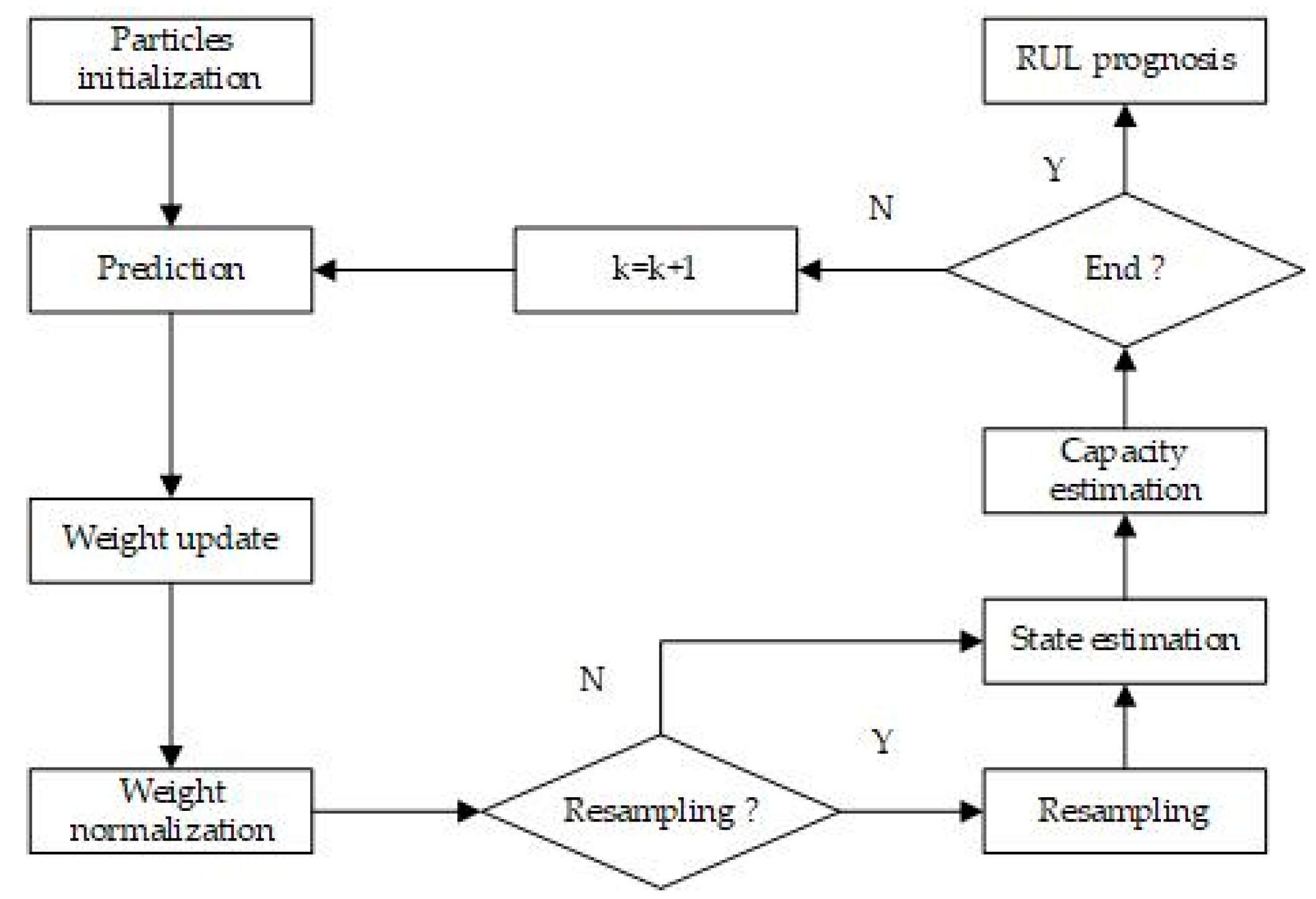
1. Particles initialization.
Suppose the initial state value is x 0 . N particles x 0 i ( i = 1 , 2 , , N ) are generated based on the prior probability density x 0 which follow a Gaussian distribution with a mean of 0 and a variance of 1 , and the weight w 0 i ( i = 1 , 2 , , N ) of each particle is 1 / N , where N is 100 in this paper.
2. Prediction.
The prediction values of the state vector and the measurement vector are predicted by Formulas (7) and (8).
3. Weight update.
Particle weights are updated according to Equations (12) and (13) [45]:
e r r k i = Q k Q ˜ k
w k i = 1 2 π R exp { ( err k i ) 2 1 2 R }
where Q ˜ k is the predicted value calculated by Equation (8) at the kth cycle, and R is 1.2668 in this paper.
4. Weight normalization.
The calculation formula of weight normalization can be expressed as [45]:
w k i = w k i i = 1 N w k i
5. Re-sampling judgement.
Calculate the number of valid samples N e f f by Equation (15) [45].
N e f f = 1 i = 1 N w k i 2
If N e f f < N t h , resampling process begins, and weight of resampled particles are 1 / N ; otherwise go directly to the next stage. Where N t h is the sampling threshold.
6. State estimation.
The state estimation calculation formula can be expressed as [45]:
x ˜ k = i = 1 N x k i w k i
7. Capacity estimation.
Each element of the state vector, obtained by the previous step, is assigned as the input weight of the ELM and the bias at each node of the hidden layer at the kth cycle. The output weight is calculated by [44]:
w = H 1 Q
Then the capacity at the kth cycle can be predicted by formula (5) and (6).
8. RUL prognosis.
RUL is the number of charge-discharge cycles that the battery capacity can withstand before the capacity failure threshold is reached for the first time. The posterior probability density (pdf) of RUL at the kth cycle can be estimated by [28]:
p ( R U L k | Q 1 : k ) = i = 1 N w k i δ ( R U L k R U L k i )
The prediction value of RUL can be estimated by [28]:
R U L k = i = 1 N w k i R U L k i
The workflow of the PFELM algorithm is shown in Figure 2.

3. Experiment and Analysis

3.1. Data Description

In this paper, the battery datasets are from datasets published by the National Aeronautics and Space Administration Ames Research Center. We selected the testing data from B0005, B0006, B0007, and B0018. The tests of these four batteries were carried out at a constant room temperature of 24 °C for the charge and discharge experiments. In the charging phase, at first, the four batteries were charged at a constant current of 1.5 A until the battery terminal voltage reached 4.2 V. Then constant voltage charging was performed until the charging current drops to 20 mA; in the discharging phase, B0005, B0006, B0007, and B0018 were discharged at a constant current of 2 A until the four terminal voltages reached 2.7 V, 2.5 V, 2.2 V, and 2.5 V, respectively. The capacity fade curves of the four batteries are shown in Figure 3. It is worth noting that MATLAB R2016a (MathWorks, Natick, MA, USA) software is used for all data processing of this paper.
In general, lithium-ion batteries are considered to be invalid when the capacity reached 80% of the initial capacity. However, in this paper, in order to verify the performance of the algorithm over a wider capacity range, we set the capacity failure thresholds of the B0005, B0006, B0007, and B0018 to 75%, 70%, 80%, and 75%of the initial capacity, respectively.

3.2. Determination of Algorithm Parameters and Evaluation Index of Results

3.2.1. Number of Layers and Nodes in Each Layer of ELM

In this paper, we chose a three-layer ELM. Three nodes were present in the input layer. Considering that the temperature is an essential factor affecting the RUL of battery [46], we took the temperature change value and the average temperature rate of change of the cell, at each discharge, as two inputs. The number of charge-discharge cycles was the third input. There was one node in the output layer, which was the output for the battery capacity. The nodes of the hidden layer were determined experimentally. The evaluation indicators of prediction results include maximum error, minimum error, mean error, and mean square error. The statistical results are shown in Table 1.
Taking into account the amount of calculations and prediction results in Table 1, we set four nodes in the hidden layer.
To ensure the equality of the external conditions, we set four hidden layer nodes in the ELM of PFELM, in the MLP of PFMLP and in the NN of BATPFNN.

3.2.2. Evaluation Index of Results

In this paper, the following three parameters were considered as results evaluation indicators of RUL prognosis.
1. Remaining Useful Life (RUL)
Remaining Useful Life (RUL) is defined as the number of charge-discharge cycles that the battery capacity can withstand before the capacity failure threshold is reached, for the first time, at a certain charge and discharge condition. It can be formulated as:
RUL = C y c l e ( Q r e a l ) C y c l e ( Q c u r r e n t )
where C y c l e ( Q r e a l ) represents the actual number of charge-discharge cycles from the current periods to the battery failure, C y c l e ( Q c u r r e n t ) represents the predicted number of charge-discharge periods from the current periods to the battery failure.
2. Absolute Error (AE)
Absolute Error (AE) is the absolute value of the difference between the predicted RUL and the real RUL, which can be formulated as:
AE = | RUL p r e d i c t i o n RUL r e a l |
where R U L p r e d i c t i o n represents the predicted RUL, R U L r e a l represents the real RUL.
3. Mean Square Error (MSE)
Mean Square Error (MSE) reflects the accuracy between the predicted capacity value and the real capacity value. The smaller the value, the better the average prognosis performance of the algorithm. It can be expressed as:
MSE = 1 M k = 1 M ( Q k Q ˜ k ) 2
where M represents the total number of cycles, Q k represents the true capacity value, Q ˜ k represents the predicted capacity value.

3.3. Experimental Results Presentation

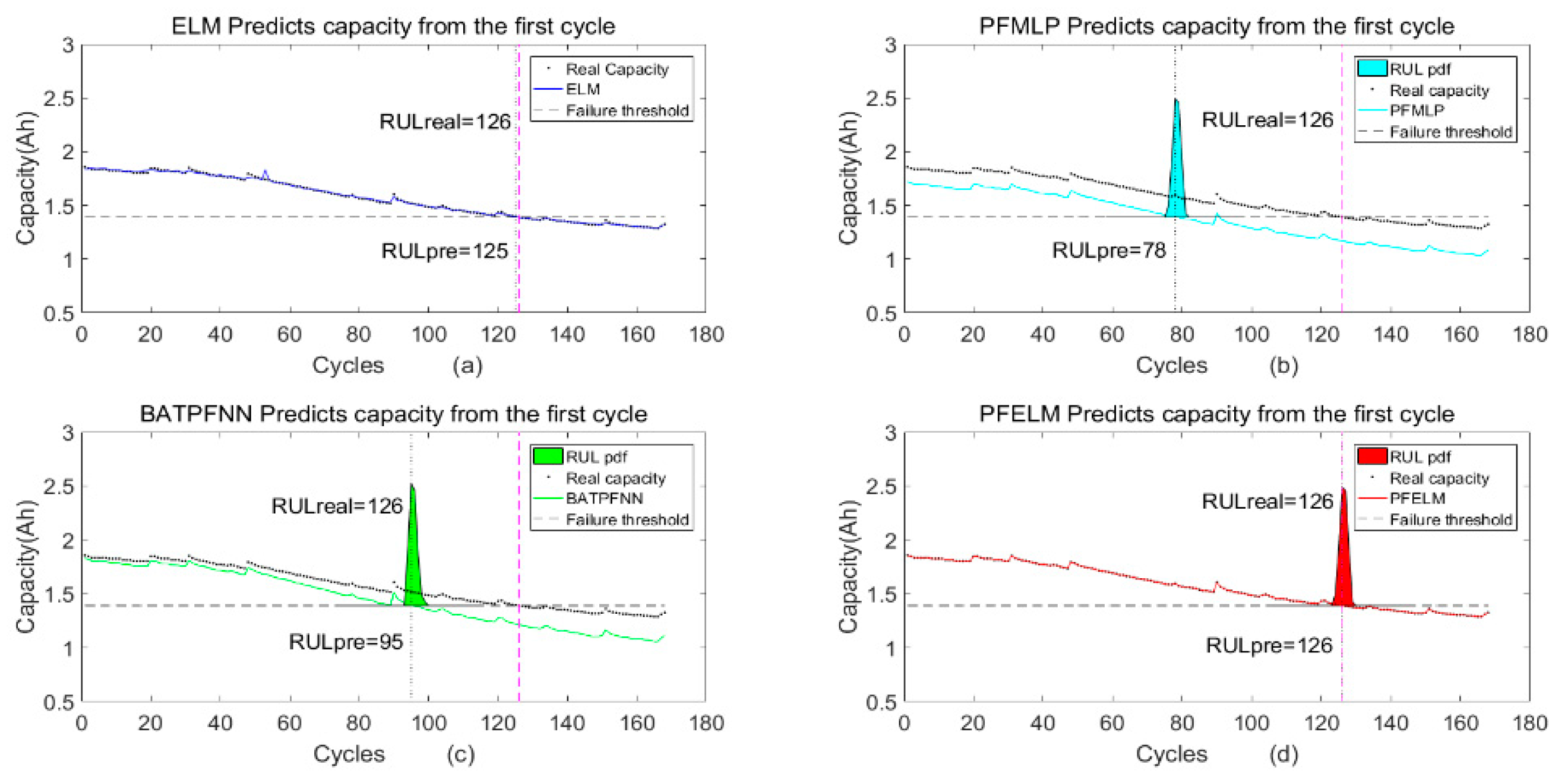
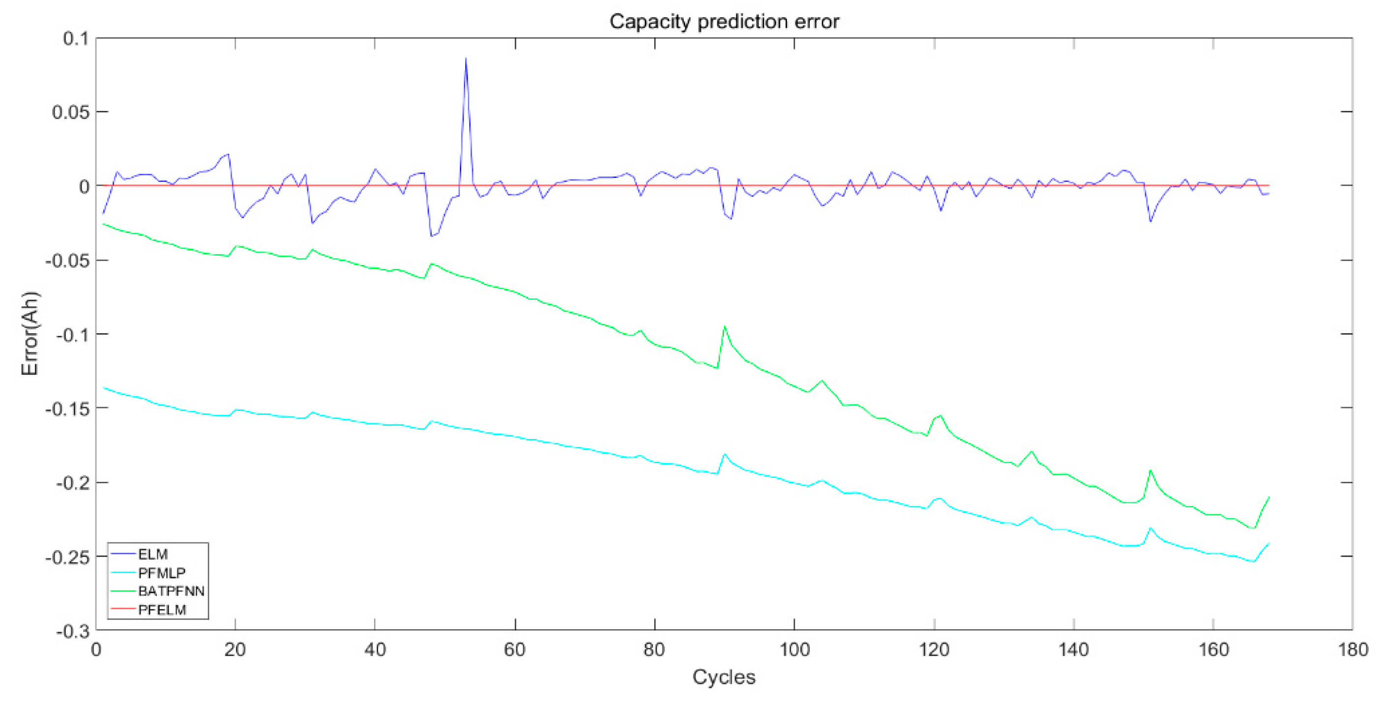
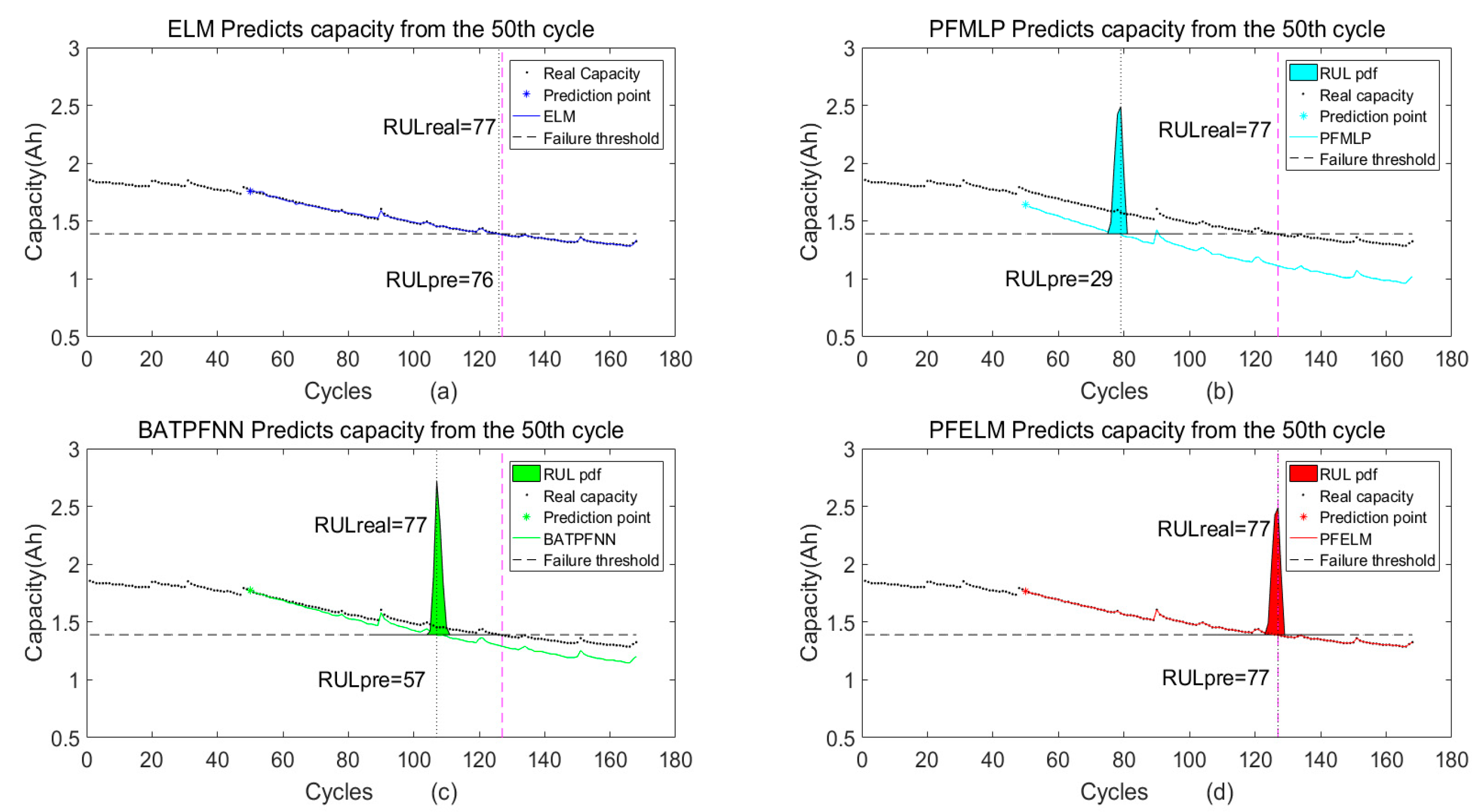
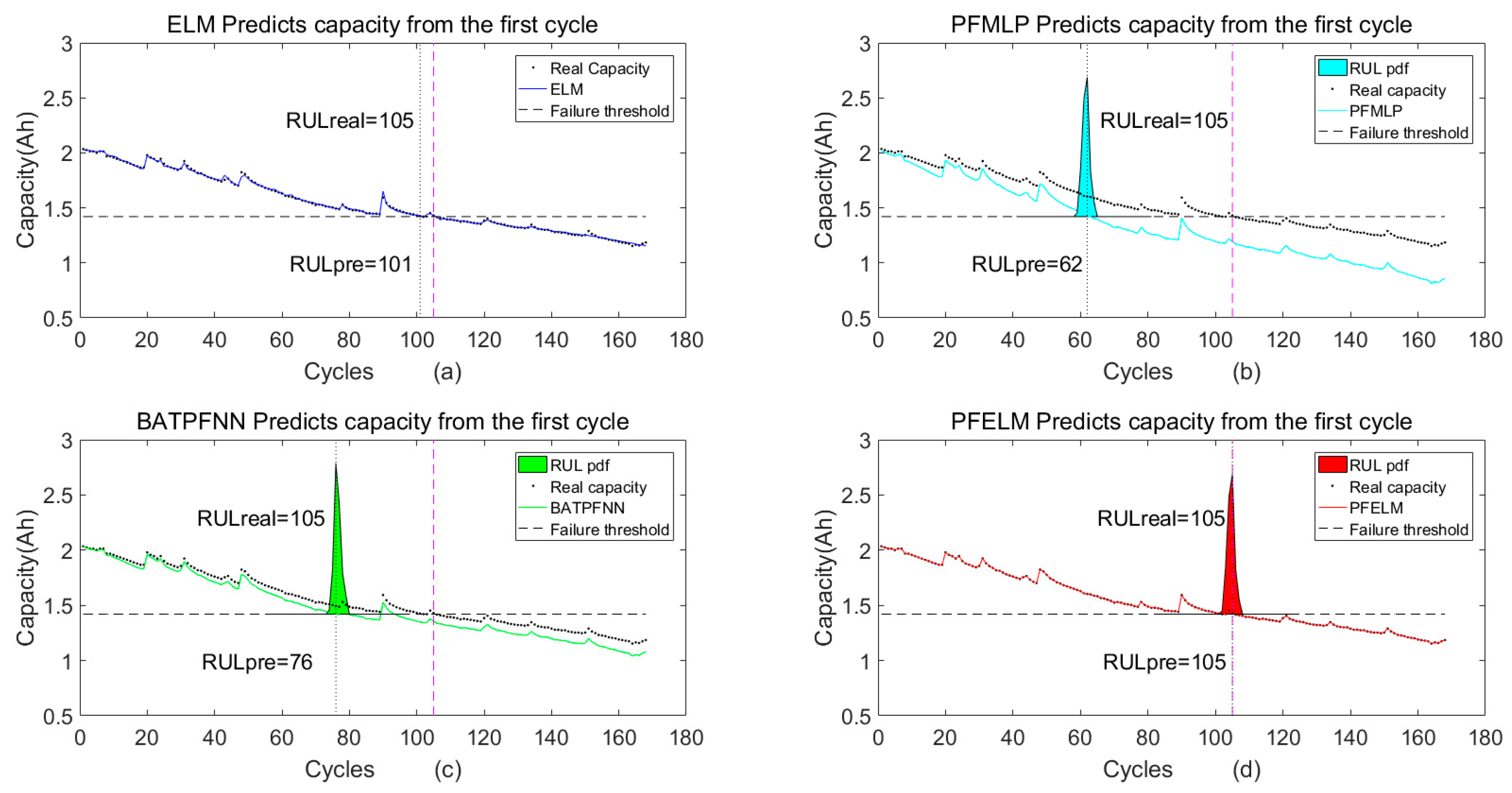
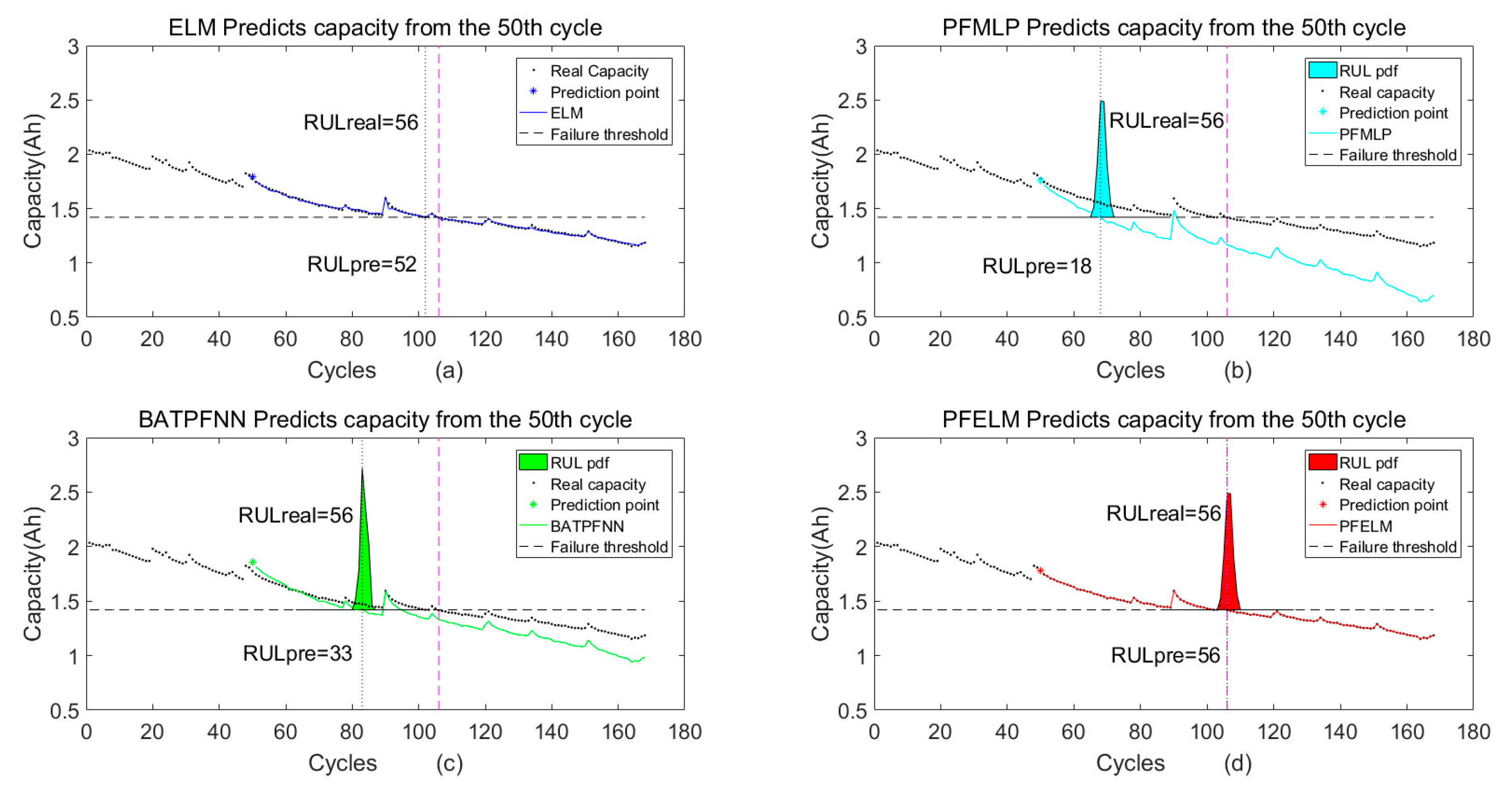
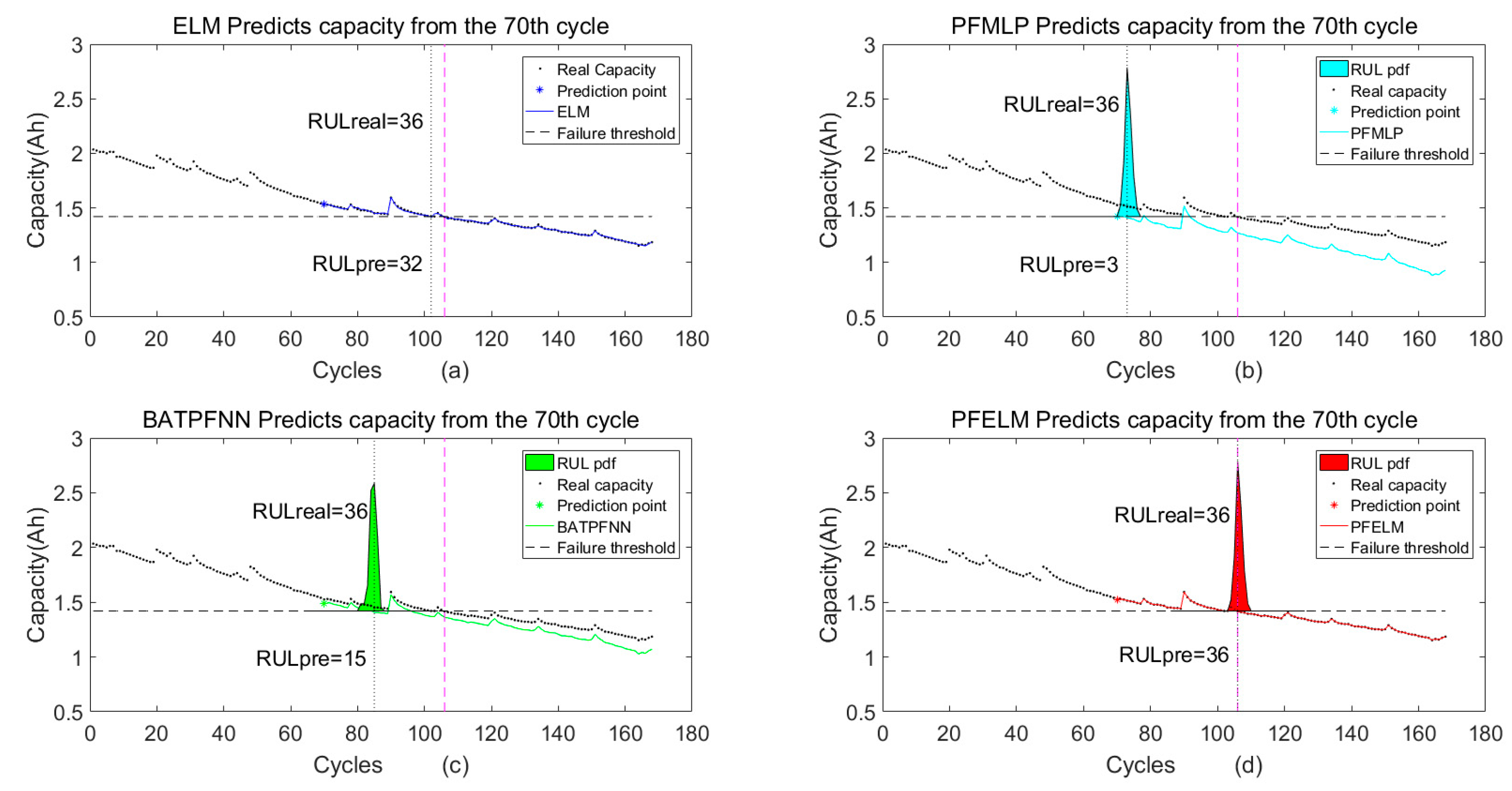
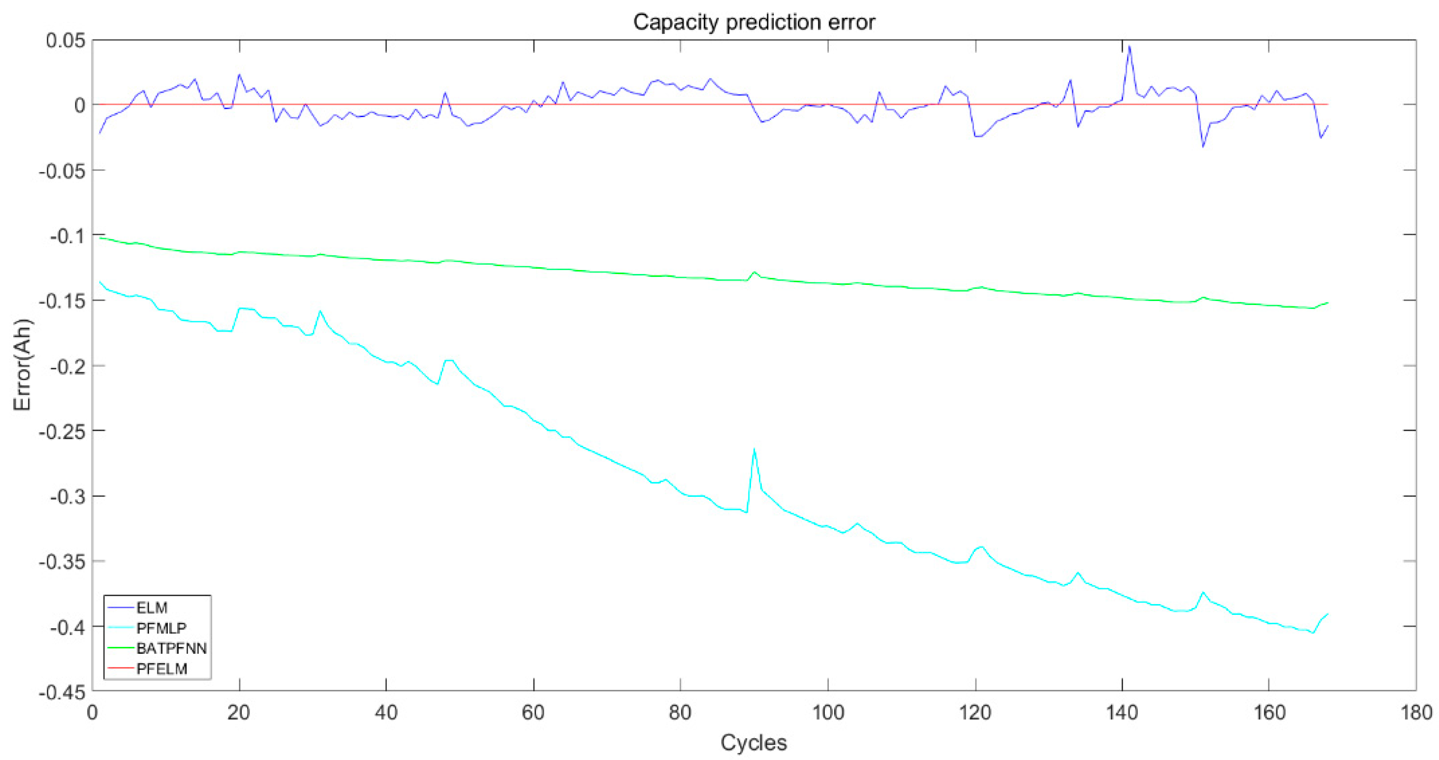
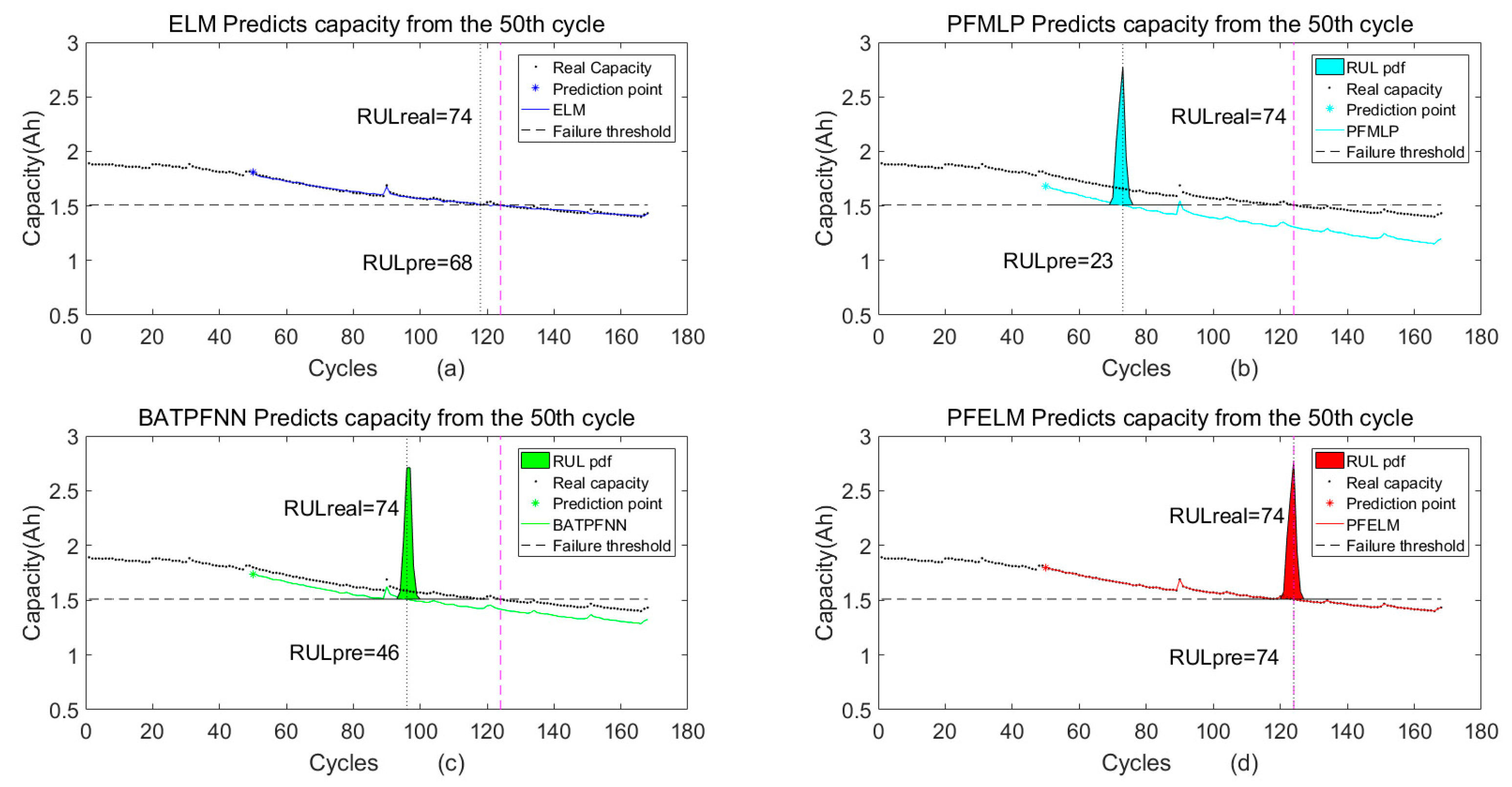
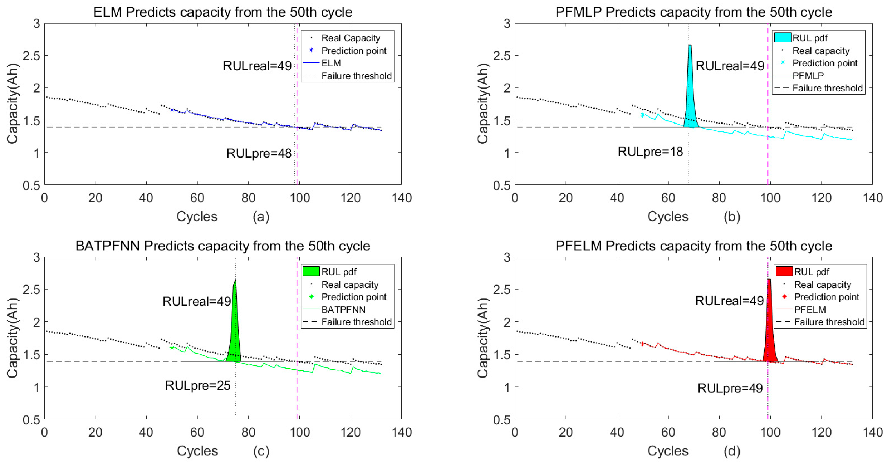
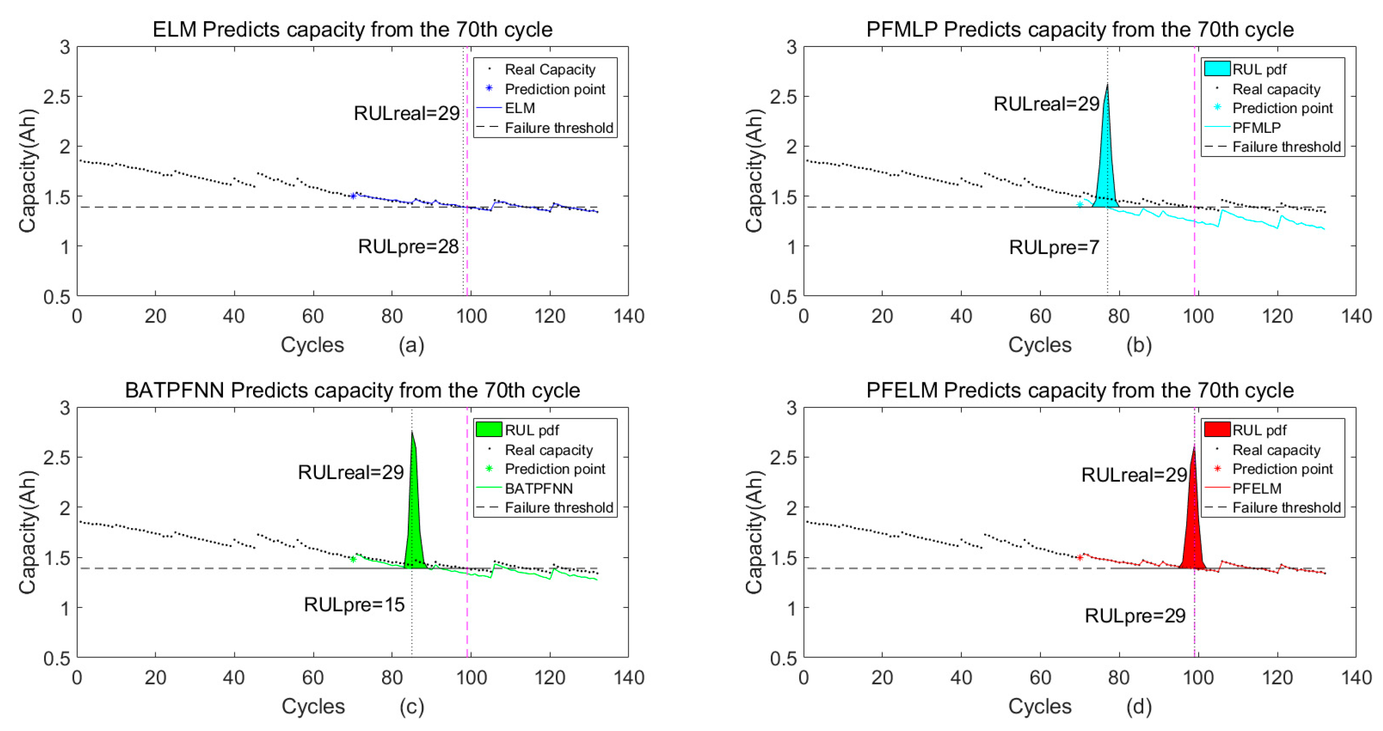
In this section, we use the batteries datasets of B0005, B0006, B0007, and B0018 from NASA Ames Research Center to test the performance of the ELM, the PFMLP, the BATPFNN, and the PFELM four algorithms. Considering the uncertainty of the starting point of the battery RUL starting prediction point in the practical operating conditions, we selected three different starting prediction points, at; 1, 50, and 70. Finally, we compared the prognosis performance of the four algorithms. Note that in all the figures in this section, the black point represented the real capacity value corresponding to each cycle, and the black dotted line parallel to the horizontal axis is the battery failure threshold line. The blue curve, cyan-blue curve, green curve and red curve are the capacity decline curves obtained by fitting the battery capacity value predicted by the ELM, the PFMLP, the BATPFNN, and the PFELM, respectively. The cyan-blue region, green region and red region represent the pdf of RUL estimated by the PFMLP, BATPFNN, and PFELM, respectively. RULreal and RULpre represent the real RUL, and the predicted RUL in all the figures in this section, respectively.

3.3.1. Comparison of Prognosis Results of B0005

From Figure 3, we can see that the initial capacity of B0005 is 1.8565 Ah, and its failure capacity value is 75% of the initial capacity.
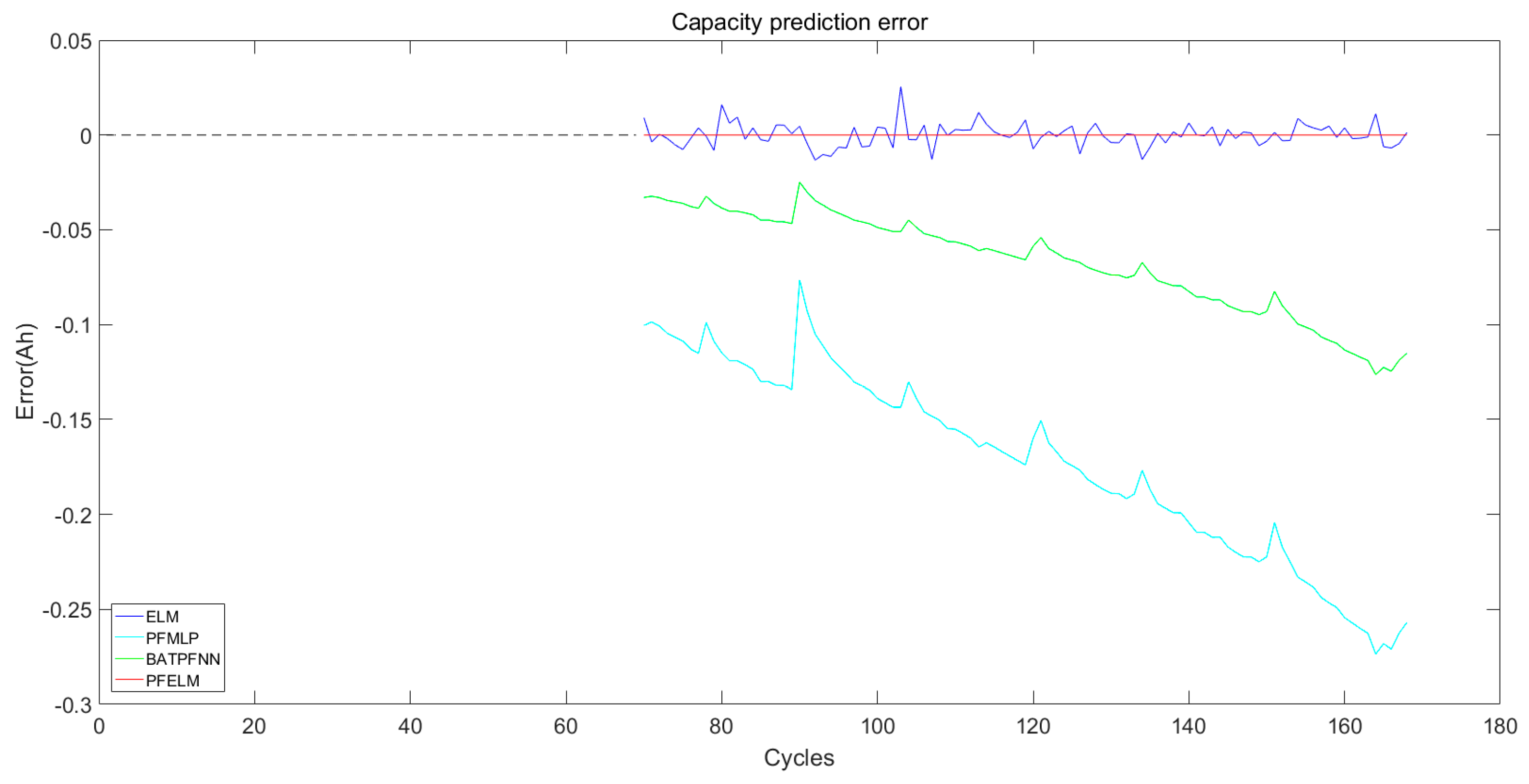
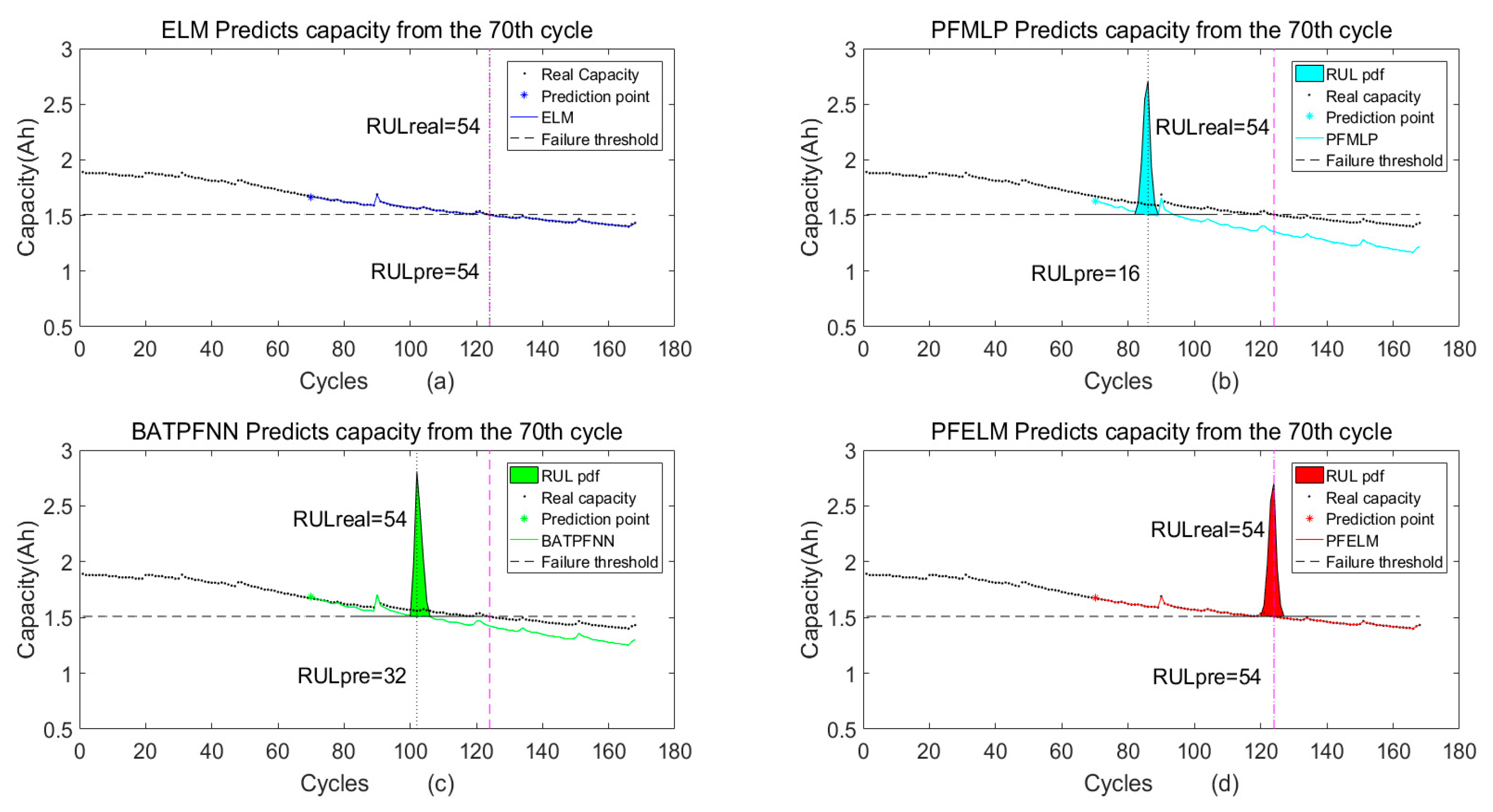
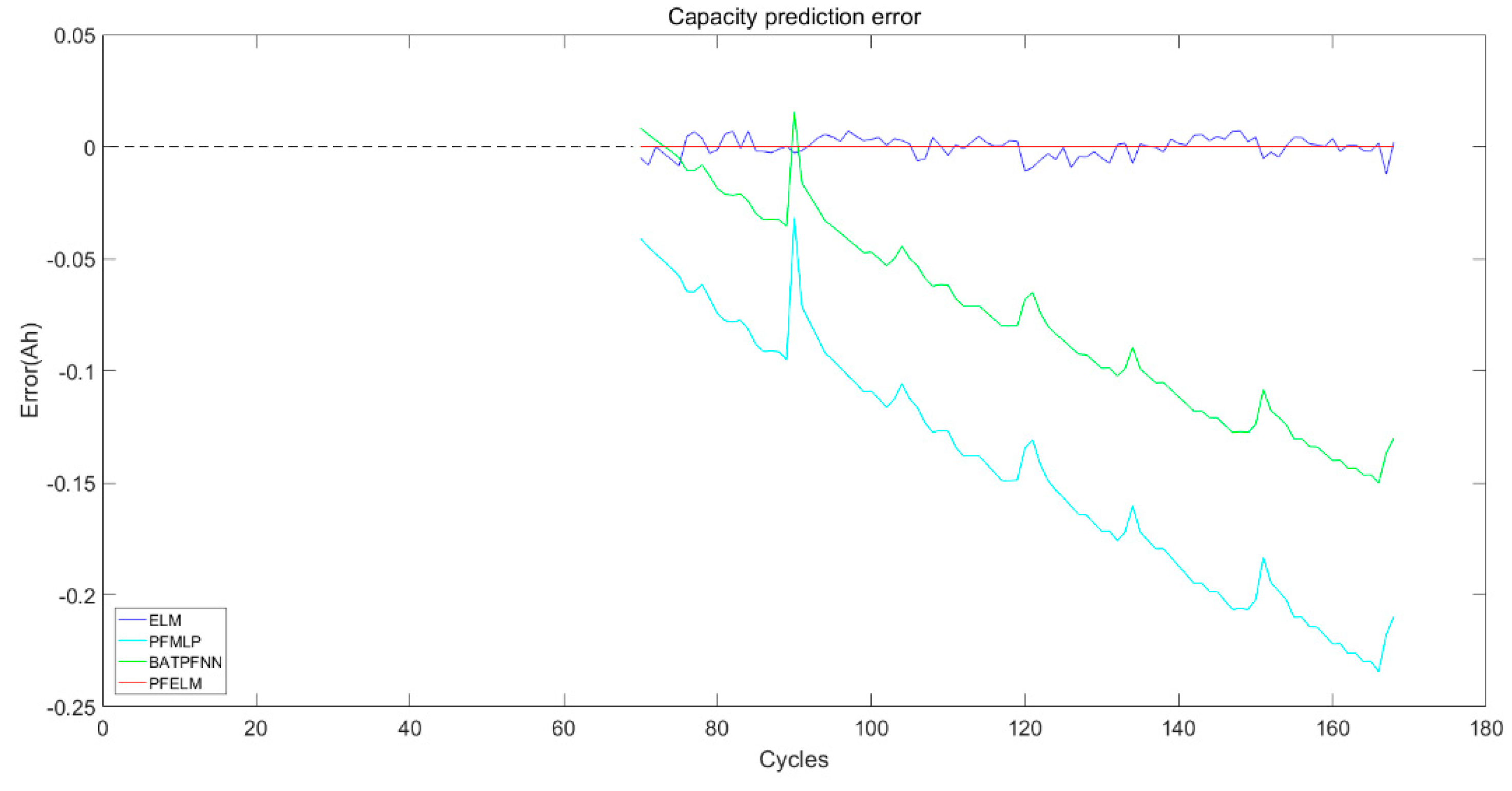
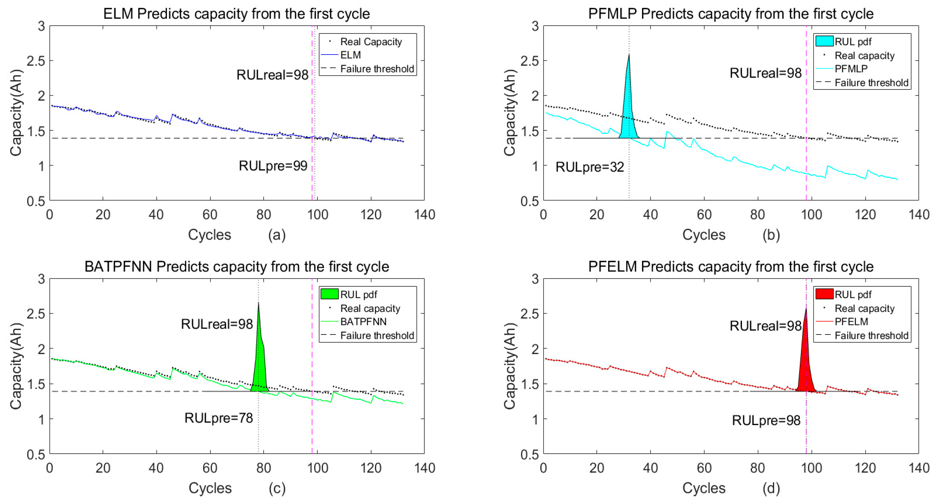
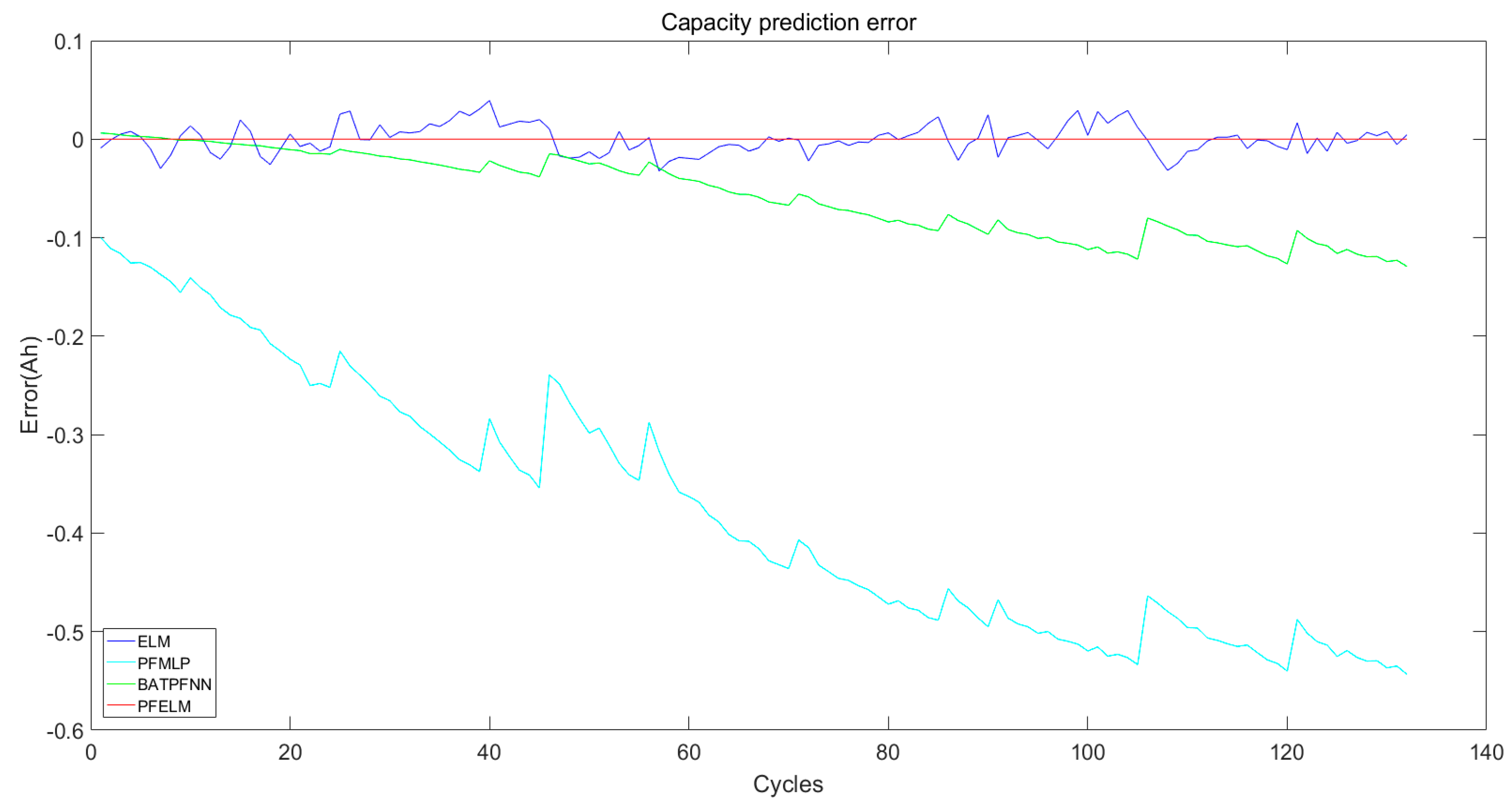
Figure 4 and Figure 5 show the predicted RUL results and capacity prediction errors starting from the first cycle, respectively. Figure 6 and Figure 7 show the predicted RUL results and capacity prediction errors starting from the 50th cycle, respectively. Figure 8 and Figure 9 show the predicted RUL results and capacity prediction errors starting from the 70th cycle, respectively. Table 2 shows the prognosis results of the four algorithms.

3.3.2. Comparison of Prognosis Results of B0006

From Figure 3, we can see that the initial capacity of B0006 is 2.0353 Ah, and its failure capacity value is 70% of the initial capacity.
Figure 10 and Figure 11 show the predicted RUL results and capacity prediction errors starting from the first cycle, respectively. Figure 12 and Figure 13 show the predicted RUL results and capacity prediction errors starting from the 50th cycle, respectively. Figure 14 and Figure 15 show the predicted RUL results and capacity prediction errors starting from the 70th cycle, respectively. Table 3 shows the prognosis results of the four algorithms.

3.3.3. Comparison of Prognosis Results of B0007

From Figure 3, we can see that the initial capacity of B0007 is 1.8911 Ah, and its failure capacity value is 80% of the initial capacity.
Figure 16 and Figure 17 show the predicted RUL results and capacity prediction errors starting from the first cycle, respectively. Figure 18 and Figure 19 show the predicted RUL results and capacity prediction errors starting from the 50th cycle, respectively. Figure 20 and Figure 21 show the predicted RUL results and capacity prediction errors starting from the 70th cycle, respectively. Table 4 shows the prognosis results of the four algorithms.

3.3.4. Comparison of Prognosis Results of B0018

From Figure 3, we can see that the initial capacity of B0018 is 1.8550 Ah, and its failure capacity value is 75% of the initial capacity.
Figure 22 and Figure 23 show the predicted RUL results and capacity prediction errors starting from the first cycle, respectively. Figure 24 and Figure 25 show the predicted RUL results and capacity prediction errors starting from the 50th cycle, respectively. Figure 26 and Figure 27 show the predicted RUL results and capacity prediction errors starting from the 70th cycle, respectively. Table 5 shows the prognosis results of the four algorithms.

3.4. Experimental Results Comparisons and Discussion

Taking the experimental results of B0005, as an example, we analyze the experimental results from two aspects: RUL prediction accuracy and robustness in detail.

3.4.1. RUL Prediction Accuracy Analysis

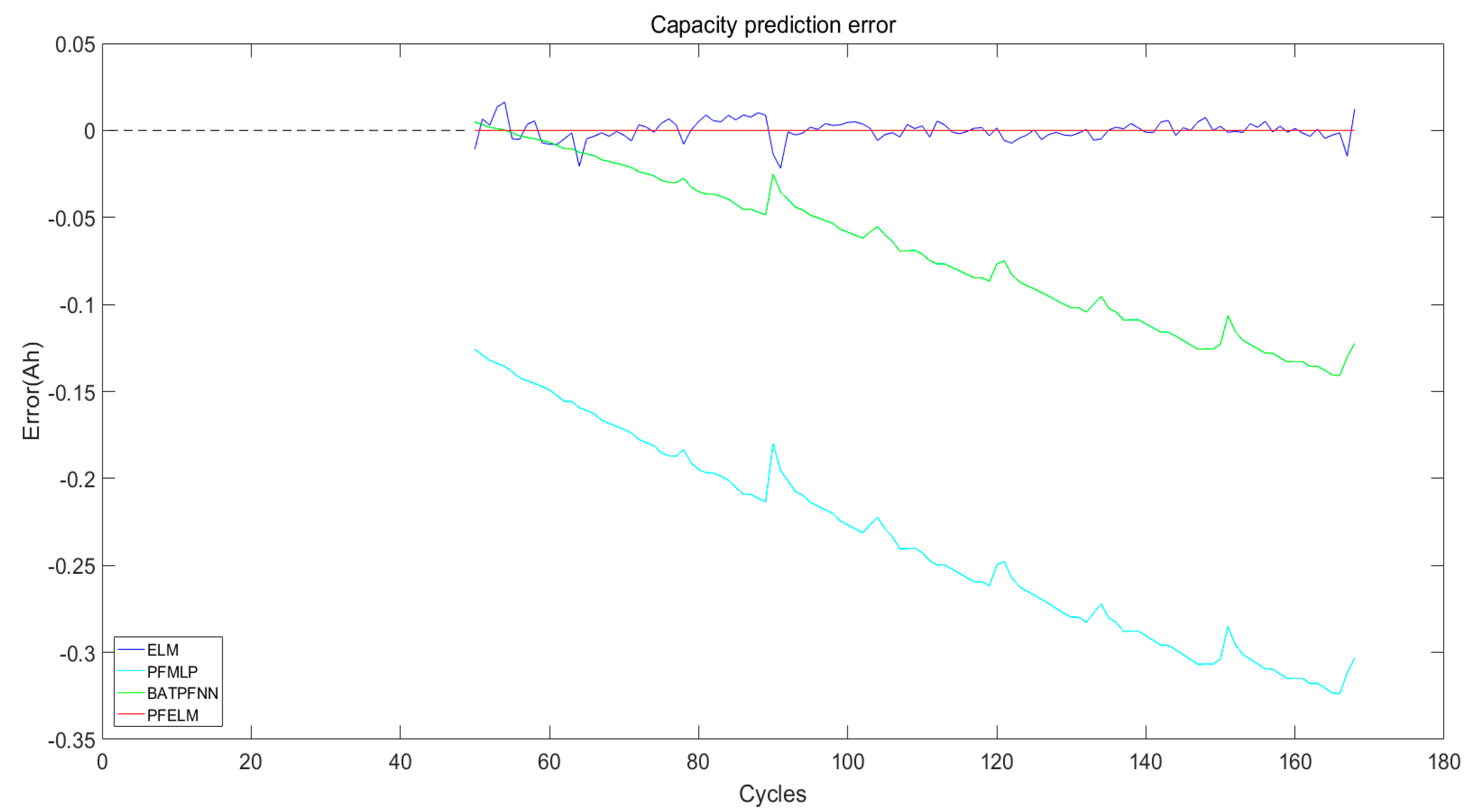
From Figure 4a, we can see that the ELM has good capacity decline tracking ability. However, the ELM cannot express uncertainty about the prediction results. According to Figure 4b,c, we can see that the BATPFNN has a better ability to track the capacity decline than the PFMLP, which is mainly due to the optimization of particles by the bat algorithm, which weakens the effect of particle degradation and impoverishment. From Figure 4 and Figure 5, it is very obvious that the capacity prediction values of the PFELM algorithm are closest to the true values and the errors are very small. The same conclusions can also be drawn from Figure 6, Figure 7, Figure 8 and Figure 9.
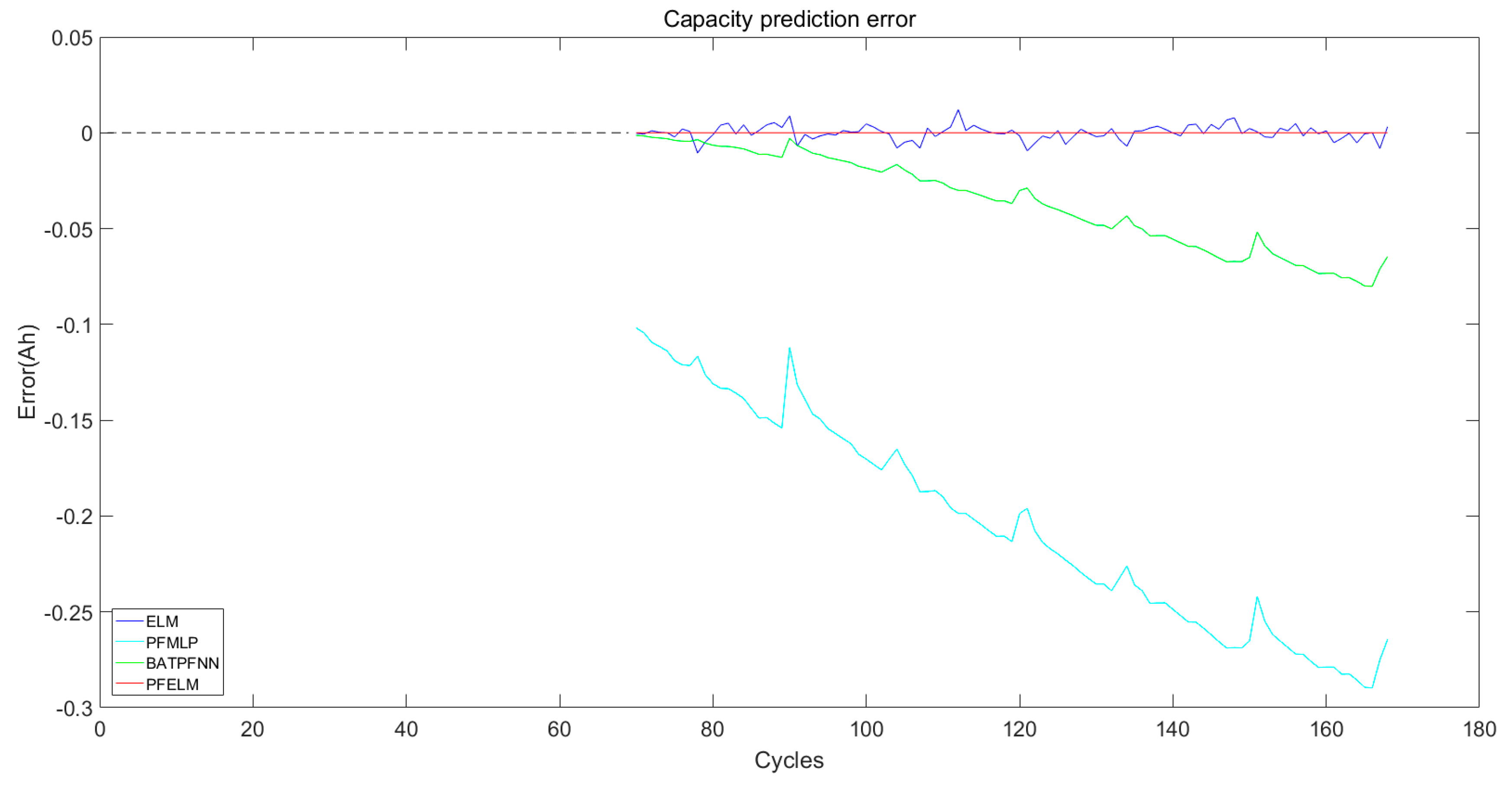
From Figure 5, Figure 7 and Figure 9, we can see that the capacity prediction error curves of the PFELM algorithm are about 0. However, the errors still exist. According to the statistical results in Table 2, there are still errors between the predicted capacity and the real capacity, but these errors are very small and have little effect on the RUL prognosis. For example, the capacity mean square error predicted by the PFELM algorithm from the 50th cycle is 3.2119 × 10⁻¹⁶, but the RUL absolute error is 0. Therefore, the PFELM algorithm has the highest capacity and RUL prediction accuracy among the four algorithms.

3.4.2. Robustness Analysis

Figure 4, Figure 6 and Figure 8 represent the capacity and RUL prediction results of the four algorithms, starting from the first cycle, the 50th cycle, and the 70th cycle, respectively. We can see the differences between the real RUL and the RUL prognosis results, by the ELM, the PFMLP, and the BATPFNN are variable when predicting from different starting cycle points. However, the RUL prediction values by the PFELM are always guaranteed to be same as the real RUL, when predicting from different cycle points, which reflects the good robustness of the PFELM algorithm.
In addition, from Figure 4, Figure 6 and Figure 8, it can be seen that the RUL pdf width and height differences, estimated by the PFMLP, the BATPFNN, and the PFELM are very small. However, the RUL pdf height by the BATPFNN is the highest among the PFMLP, the BATPFNN, and the PFELM three algorithms, because the extent of particle impoverishment is weakened due to the introduction of the bat algorithm. However, the RUL pdf width and height are not the concern of this paper. Particle impoverishment does not affect the accuracy of RUL estimation from the current experimental results. Therefore, we do not make redundant introductions.
The same conclusions can also be drawn from experimental results of B0006, B0007, and B0018. Therefore, we can conclude that the PFELM algorithm can provide more accurate RUL estimation for B0005, B0006, B0007, and B0018.

4. Conclusions

In this paper, we presented a novel hybrid method for particle filter based extreme learning machine for RUL estimation of lithium ion batteries. And the results predicted by the ELM, the PFMLP, the BATPFNN, and the PFELM has been analyzed in detail. The results show that, compared with ELM, PFMLP, BAPFNN algorithm, (1) the PFELM algorithm has lower capacity prediction error and higher RUL prediction accuracy; (2) the PFELM algorithm can provide accurate and stable RUL prognosis results predicting from different starting cycle points, which indicates that the PFELM algorithm has better robustness.
Although the proposed PAFELM algorithm perform good RUL prognostic effect. However, the universality of the PFELM algorithm remains to be verified. Different types of batteries have different capacity degradation behaviors, under different operating conditions, such as the ambient temperature, the discharge current, and the depth of discharge. Besides, the state initial values, the process noise, and the measurement noise are the potential factors that influence the PFELM algorithm prediction accuracy and robustness. Therefore, finding the factors of affecting the algorithm prediction accuracy and exploring whether the PFELM algorithm is universal, will be investigated in our next research.

Author Contributions

T.S. and B.X. proposed the method and analyzed the results; Y.L. (Yifan Liu), Y.L. (Yongzhi Lai), W.Z., H.W., W.W., and M.W. obtained the capacity datasets and processed them. T.S. wrote the paper.

Funding

This research was funded by the Shenzhen Economic, Trade and Information Commission of Shenzhen. Municipality Strategic Emerging Industries and Future Industrial Development “Innovation Chain + Industrial. Chain” Project (2017), and National Natural Science Foundation of China (Grant No. 51877120).

Conflicts of Interest

The authors declare no conflict of interest.

References

  1. Rodrigues, E.M.G.; Godina, R.; Catalao, J.P.S. Modelling electrochemical energy storage devices in insular power network applications supported on real data. Appl. Energy 2017, 188, 315–329. [Google Scholar] [CrossRef]
  2. Menale, C.; D’Annibale, F.; Mazzarotta, B.; Bubbico, R. Thermal management of lithium-ion batteries: An experimental investigation. Energy 2019, 182, 57–71. [Google Scholar] [CrossRef]
  3. Li, F.; Xu, J.P. A new prognostics method for state of health estimation of lithium-ion batteries based on a mixture of Gaussian process models and particle filter. Microelectron. Reliab. 2015, 55, 1035–1045. [Google Scholar] [CrossRef]
  4. Nuhic, A.; Terzimehic, T.; Soczka-Guth, T.; Buchholz, M.; Dietmayer, K. Health diagnosis and remaining useful life prognostics of lithium-ion batteries using data-driven methods. J. Power Sources 2013, 239, 680–688. [Google Scholar] [CrossRef]
  5. Wu, L.F.; Fu, X.H.; Guan, Y. Review of the Remaining Useful Life Prognostics of Vehicle Lithium-Ion Batteries Using Data-Driven Methodologies. Appl. Sci. 2016, 6, 166. [Google Scholar] [CrossRef]
  6. Barre, A.; Deguilhem, B.; Grolleau, S.; Gerard, M.; Suard, F.; Riu, D. A review on lithium-ion battery ageing mechanisms and estimations for automotive applications. J. Power Sources 2013, 241, 680–689. [Google Scholar] [CrossRef] [Green Version]
  7. Su, C.; Chen, H.J. A review on prognostics approaches for remaining useful life of lithium-ion battery. In Proceedings of the 2017 International Conference on New Energy and Future Energy System, Kunming, China, 22–25 September 2017; Kyriakopoulos, G.L., Ed.; Iop Publishing Ltd.: Bristol, UK, 2017; Volume 93. [Google Scholar]
  8. Jirkof, P.; Schmutz, J.B. Social and organizational factors affecting biosafety compliance in animal facilities: An integrative analysis of safety rules within the system. Saf. Sci. 2019, 118, 538–550. [Google Scholar] [CrossRef]
  9. Qu, S.; Kang, Y.; Gu, P.; Zhang, C.; Duan, B. A Fast Online State of Health Estimation Method for Lithium-Ion Batteries Based on Incremental Capacity Analysis. Energies 2019, 12, 3333. [Google Scholar] [CrossRef]
  10. Su, X.H.; Wang, S.; Pecht, M.; Ma, P.J.; Zhao, L.L. Prognostics of lithium-ion batteries based on different dimensional state equations in the particle filtering method. Trans. Inst. Meas. Control 2017, 39, 1537–1546. [Google Scholar] [CrossRef]
  11. Liu, D.T.; Yin, X.H.; Song, Y.C.; Liu, W.; Peng, Y. An On-Line State of Health Estimation of Lithium-Ion Battery Using Unscented Particle Filter. IEEE Access 2018, 6, 40990–41001. [Google Scholar] [CrossRef]
  12. Liu, Z.B.; Fan, D.S.; Bu, S.H.; Zhang, C. Prediction of Remaining Useful Life of Battery Cell Using Logistic Regression Based on Strong Tracking Particle Filter. In Proceedings of the 2015 IEEE Conference on Prognostics and Health Management (PHM), Austin, TX, USA, 22–25 June 2015. [Google Scholar]
  13. Mo, B.H.; Yu, J.S.; Tang, D.Y.; Liu, H.; Yu, J.S. A remaining useful life prediction approach for lithium-ion batteries using Kalman filter and an improved particle filter. In Proceedings of the 2016 IEEE International Conference on Prognostics and Health Management (ICPHM), Ottawa, ON, Canada, 20–22 June 2016. [Google Scholar]
  14. He, W.; Pecht, M.; Flynn, D.; Dinmohammadi, F. A Physics-Based Electrochemical Model for Lithium-Ion Battery State-of-Charge Estimation Solved by an Optimised Projection-Based Method and Moving-Window Filtering. Energies 2018, 11, 23. [Google Scholar] [CrossRef]
  15. Andre, D.; Appel, C.; Soczka-Guth, T.; Sauer, D.U. Advanced mathematical methods of SOC and SOH estimation for lithium-ion batteries. J. Power Sources 2013, 224, 20–27. [Google Scholar] [CrossRef]
  16. Xu, X.D.; Yu, C.Q.; Tang, S.J.; Sun, X.Y.; Si, X.S.; Wu, L.F. Remaining Useful Life Prediction of Lithium-Ion Batteries Based on Wiener Processes with Considering the Relaxation Effect. Energies 2019, 12, 17. [Google Scholar] [CrossRef]
  17. Wu, J.; Zhang, C.B.; Chen, Z.H. An online method for lithium-ion battery remaining useful life estimation using importance sampling and neural networks. Appl. Energy 2016, 173, 134–140. [Google Scholar] [CrossRef]
  18. Choi, H.S.; Cho, W.J. Investigation of Multi-Level Cell Characteristic in Amorphous Indium-Gallium-Zinc Oxide Thin-Film-Transistor Based 1T-1R Non-Volatile Memory Device. J. Nanosci. Nanotechnol. 2019, 19, 6031–6035. [Google Scholar] [CrossRef] [PubMed]
  19. Long, B.; Li, X.; Gao, X.; Liu, Z. Prognostics Comparison of Lithium-Ion Battery Based on the Shallow and Deep Neural Networks Model. Energies 2019, 12, 3271. [Google Scholar] [CrossRef]
  20. Pang, X.Q.; Huang, R.; Wen, J.; Shi, Y.H.; Jia, J.F.; Zeng, J.C. A Lithium-ion Battery RUL Prediction Method Considering the Capacity Regeneration Phenomenon. Energies 2019, 12, 14. [Google Scholar] [CrossRef]
  21. Li, X.Y.; Shu, X.; Shen, J.W.; Xiao, R.X.; Yan, W.S.; Chen, Z. An On-Board Remaining Useful Life Estimation Algorithm for Lithium-Ion Batteries of Electric Vehicles. Energies 2017, 10, 15. [Google Scholar] [CrossRef]
  22. Liu, D.T.; Zhou, J.B.; Pan, D.W.; Peng, Y.; Peng, X.Y. Lithium-ion battery remaining useful life estimation with an optimized Relevance Vector Machine algorithm with incremental learning. Measurement 2015, 63, 143–151. [Google Scholar] [CrossRef]
  23. Severson, K.A.; Attia, P.M.; Jin, N.; Perkins, N.; Jiang, B.; Yang, Z.; Chen, M.H.; Aykol, M.; Herring, P.K.; Fraggedakis, D.; et al. Data-driven prediction of battery cycle life before capacity degradation. Nat. Energy 2019, 4, 383–391. [Google Scholar] [CrossRef] [Green Version]
  24. Khumprom, P.; Yodo, N. A Data-Driven Predictive Prognostic Model for Lithium-ion Batteries based on a Deep Learning Algorithm. Energies 2019, 12, 21. [Google Scholar] [CrossRef]
  25. Long, B.; Xian, W.M.; Jiang, L.; Liu, Z. An improved autoregressive model by particle swarm optimization for prognostics of lithium-ion batteries. Microelectron. Reliab. 2013, 53, 821–831. [Google Scholar] [CrossRef]
  26. Liu, J.; Chen, Z.Q. Remaining Useful Life Prediction of Lithium-Ion Batteries Based on Health Indicator and Gaussian Process Regression Model. IEEE Access 2019, 7, 39474–39484. [Google Scholar] [CrossRef]
  27. Cadini, F.; Sbarufatti, C.; Cancelliere, F.; Giglio, M. State-of-life prognosis and diagnosis of lithium-ion batteries by data-driven particle filters. Appl. Energy 2019, 235, 661–672. [Google Scholar] [CrossRef]
  28. Wu, Y.; Li, W.; Wang, Y.R.; Zhang, K. Remaining Useful Life Prediction of Lithium-Ion Batteries Using Neural Network and Bat-Based Particle Filter. IEEE Access 2019, 7, 54843–54854. [Google Scholar] [CrossRef]
  29. Wei, J.W.; Dong, G.Z.; Chen, Z.H. Remaining Useful Life Prediction and State of Health Diagnosis for Lithium-Ion Batteries Using Particle Filter and Support Vector Regression. IEEE Trans. Ind. Electron. 2018, 65, 5634–5643. [Google Scholar] [CrossRef]
  30. Chang, Y.; Fang, H.J. A hybrid prognostic method for system degradation based on particle filter and relevance vector machine. Reliab. Eng. Syst. Saf. 2019, 186, 51–63. [Google Scholar] [CrossRef]
  31. Sbarufatti, C.; Corbetta, M.; Giglio, M.; Cadini, F. Adaptive prognosis of lithium-ion batteries based on the combination of particle filters and radial basis function neural networks. J. Power Sources 2017, 344, 128–140. [Google Scholar] [CrossRef]
  32. Zhao, L.; Wang, Y.P.; Cheng, J.H. A Hybrid Method for Remaining Useful Life Estimation of Lithium-Ion Battery with Regeneration Phenomena. Appl. Sci. 2019, 9, 15. [Google Scholar] [CrossRef]
  33. Si, X.S. An Adaptive Prognostic Approach via Nonlinear Degradation Modeling: Application to Battery Data. IEEE Trans. Ind. Electron. 2015, 62, 5082–5096. [Google Scholar] [CrossRef]
  34. Yang, J.; Peng, Z.; Pei, Z.D.; Guan, Y.; Yuan, H.M.; Wu, L.F. Remaining Useful Life Assessment of Lithium-ion Battery based on HKA-ELM Algorithm. Int. J. Electrochem. Sci. 2018, 13, 9257–9272. [Google Scholar] [CrossRef]
  35. Ma, Y.Y.; Shen, D.X.; Wu, L.F.; Guan, Y.; Zhu, H. The Remaining Useful Life Estimation of Lithium-ion Batteries Based on the HKA -ML-ELM Algorithm. Int. J. Electrochem. Sci. 2019, 14, 7737–7757. [Google Scholar] [CrossRef]
  36. Huang, G.B.; Zhu, Q.Y.; Siew, C.K. Extreme learning machine: A new learning scheme of feedforward neural networks. In Proceedings of the 2004 IEEE International Joint Conference on Neural Networks, Budapest, Hungary, 25–29 July 2004; Volume 1–4, pp. 985–990. [Google Scholar]
  37. Huang, G.B.; Chen, L.; Siew, C.K. Universal approximation using incremental constructive feedforward networks with random hidden nodes. IEEE Trans. Neural Netw. 2006, 17, 879–892. [Google Scholar] [CrossRef] [PubMed]
  38. Huang, G.B.; Chen, L. Convex incremental extreme learning machine. Neurocomputing 2007, 70, 3056–3062. [Google Scholar] [CrossRef]
  39. Huang, G.B.; Chen, L. Enhanced random search based incremental extreme learning machine. Neurocomputing 2008, 71, 3460–3468. [Google Scholar] [CrossRef]
  40. Kumar, S.; Pal, S.K.; Singh, R. A novel hybrid model based on particle swarm optimisation and extreme learning machine for short-term temperature prediction using ambient sensors. Sustain. Cities Soc. 2019, 49, 12. [Google Scholar] [CrossRef]
  41. Li, G.Q.; Chen, B.; Qi, X.B.; Zhang, L. Circular convolution parallel extreme learning machine for modeling boiler efficiency for a 300 MW CFBB. Soft Comput. 2019, 23, 6567–6577. [Google Scholar] [CrossRef]
  42. Lin, P.C.; Huang, H.C.; Komorowski, M.; Lin, W.K.; Changh, C.M.; Chen, K.T.; Li, Y.C.; Lin, M.C. A machine learning approach for predicting urine output after fluid administration. Comput. Meth. Programs Biomed. 2019, 177, 155–159. [Google Scholar] [CrossRef]
  43. You, Z.H.; Lei, Y.K.; Zhu, L.; Xia, J.F.; Wang, B. Prediction of protein-protein interactions from amino acid sequences with ensemble extreme learning machines and principal component analysis. BMC Bioinform. 2013, 14, 11. [Google Scholar] [CrossRef]
  44. Huang, G.B. An Insight into Extreme Learning Machines: Random Neurons, Random Features and Kernels. Cogn. Comput. 2014, 6, 376–390. [Google Scholar] [CrossRef]
  45. Xia, B.Z.; Guo, S.K.; Wang, W.; Lai, Y.Z.; Wang, H.W.; Wang, M.W.; Zheng, W.W. A State of Charge Estimation Method Based on Adaptive Extended Kalman-Particle Filtering for Lithium-ion Batteries. Energies 2018, 11, 15. [Google Scholar] [CrossRef]
  46. Su, L.S.; Zhang, J.B.; Wang, C.J.; Zhang, Y.K.; Li, Z.; Song, Y.; Jin, T.; Ma, Z. Identifying main factors of capacity fading in lithium ion cells using orthogonal design of experiments. Appl. Energy 2016, 163, 201–210. [Google Scholar] [CrossRef]
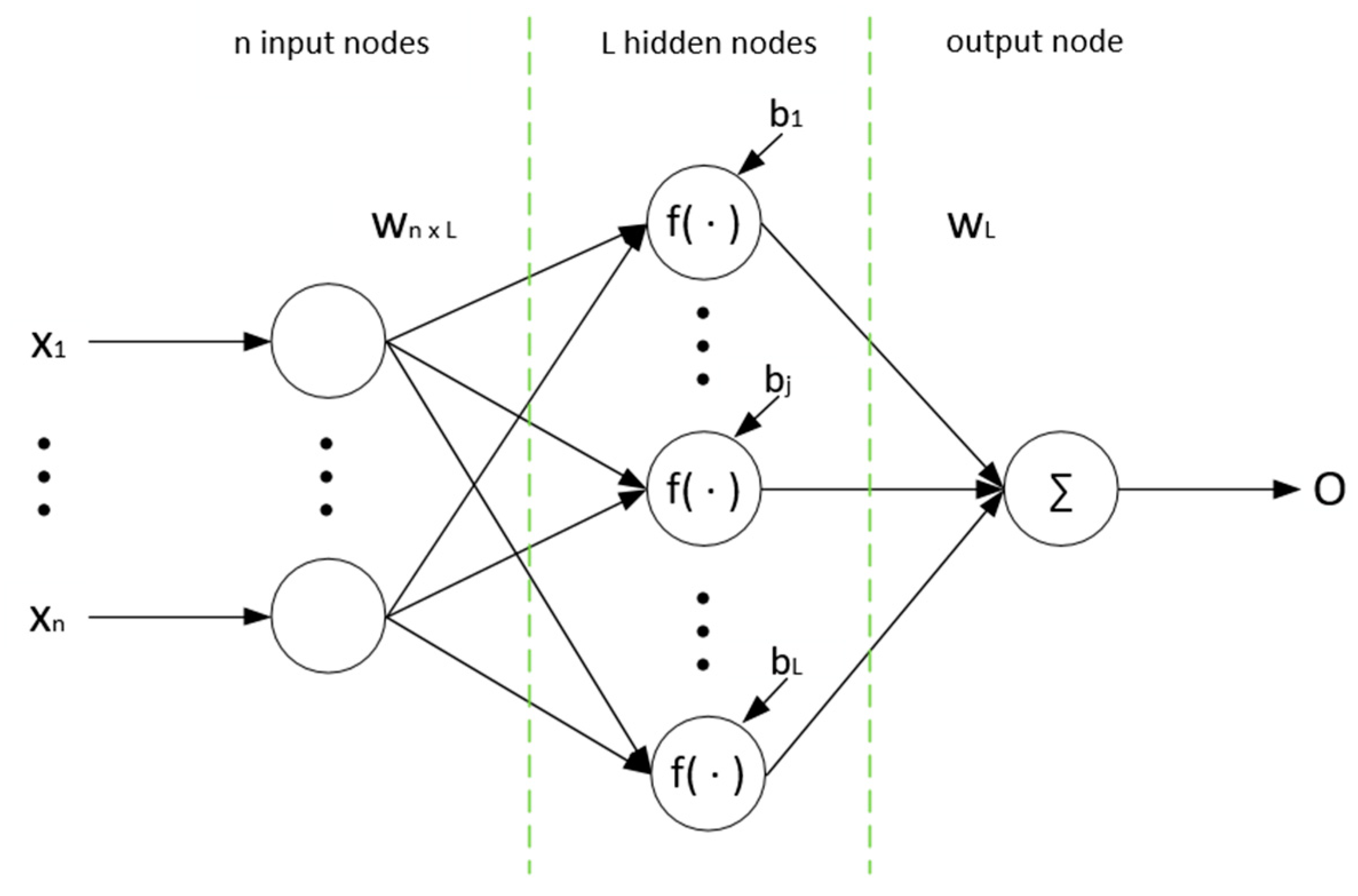
Figure 1. Structure of a single hidden layer and single output extreme learning machine (ELM).
Energies 12 03678 g001
Figure 2. Prognosis process of the particle filter based extreme learning machine (PFELM) algorithm.
Energies 12 03678 g002
Figure 3. Capacity fade curves of B0005, B0006, B0007, and B0018.
Energies 12 03678 g003
Figure 4. Predicting capacity from the first cycle by different algorithms: (a) ELM; (b) perceptron prognosis model-based on particle filter (PFMLP); (c) BATPFNN; (d) PFELM.
Energies 12 03678 g004
Figure 5. Capacity prediction error from the first cycle.
Energies 12 03678 g005
Figure 6. Predicting capacity from the 50th cycle by different algorithms: (a) ELM; (b) PFMLP; (c) BATPFNN; (d) PFELM.
Energies 12 03678 g006
Figure 7. Capacity prediction error from the 50th cycle.
Energies 12 03678 g007
Figure 8. Predicting capacity from the 70th cycle by different algorithms: (a) ELM; (b) PFMLP; (c) BATPFNN; (d) PFELM.
Energies 12 03678 g008
Figure 9. Capacity prediction error from the 70th cycle.
Energies 12 03678 g009
Figure 10. Predicting capacity from the first cycle by different algorithms: (a) ELM; (b) PFMLP; (c) BATPFNN; (d) PFELM.
Energies 12 03678 g010
Figure 11. Capacity prediction error from the first cycle.
Energies 12 03678 g011
Figure 12. Predicting capacity from the 50th cycle by different algorithms: (a) ELM; (b) PFMLP; (c) BATPFNN; (d) PFELM.
Energies 12 03678 g012
Figure 13. Capacity prediction error from the 50th cycle.
Energies 12 03678 g013
Figure 14. Predicting capacity from the first cycle by different algorithms: (a) ELM; (b) PFMLP; (c) BATPFNN; (d) PFELM.
Energies 12 03678 g014
Figure 15. Capacity prediction error from the 70th cycle.
Energies 12 03678 g015
Figure 16. Predicting capacity from the first cycle by different algorithms: (a) ELM; (b) PFMLP; (c) BATPFNN; (d) PFELM.
Energies 12 03678 g016
Figure 17. Capacity prediction error from the first cycle.
Energies 12 03678 g017
Figure 18. Predicting capacity from the 50th cycle by different algorithms: (a) ELM; (b) PFMLP; (c) BATPFNN; (d) PFELM.
Energies 12 03678 g018
Figure 19. Capacity prediction error from the 50th cycle.
Energies 12 03678 g019
Figure 20. Predicting capacity from the 50th cycle by different algorithms: (a) ELM; (b) PFMLP; (c) BATPFNN; (d) PFELM.
Energies 12 03678 g020
Figure 21. Capacity prediction error from the 70th cycle.
Energies 12 03678 g021
Figure 22. Predicting capacity from the first cycle by different algorithms: (a) ELM; (b) PFMLP; (c) BATPFNN; (d) PFELM.
Energies 12 03678 g022
Figure 23. Capacity prediction error from the first cycle.
Energies 12 03678 g023
Figure 24. Predicting capacity from the 50th cycle by different algorithms: (a) ELM; (b) PFMLP; (c) BATPFNN; (d) PFELM.
Energies 12 03678 g024
Figure 25. Capacity prediction error from the 50th cycle.
Energies 12 03678 g025
Figure 26. Predicting capacity from the 70th cycle by different algorithms: (a) ELM; (b) PFMLP; (c) BATPFNN; (d) PFELM.
Energies 12 03678 g026
Figure 27. Capacity prediction error from the 70th cycle.
Energies 12 03678 g027
Table 1. Capacity prediction results of different hidden layer nodes number.
LMaximum ErrorMinimum Error Average Error Mean Square Error
30.059−0.07600.018
40.032−0.044 0 0.013
50.052−0.0380 0.015
60.044−0.0440 0.012
70.045−0.03700.013
80.037−0.03900.013
90.048−0.05200.016
100.030−0.02500.010
Table 2. Comparison of Prognosis Results of B0005.
Prediction PointReal RULMethod Predicted RULAE MSERUL Pdf Range
1126ELM12510.0111None
PFMLP78480.1949[76,81]
BATPFNN 95310.1338[94,99]
PFELM12602.9424 × 10−16[124,129]
5077ELM7610.0058None
PFMLP 29480.2431[76,80]
BATPFNN57200.0818[105,110]
PFELM7703.2119 × 10−16[124,128]
7057ELM5610.0038None
PFMLP 16410.2111[84,89]
BATPFNN46110.0438[112,118]
PFELM5703.0353 × 10−16[125,130]
Table 3. Comparison of Prognosis Results of B0006.
Prediction PointReal RULMethod Predicted RUL AE MSERUL Pdf Range
1105ELM10140.0110None
PFMLP 62430.2169[59,64]
BATPFNN76290.0710[74–79]
PFELM10503.2414 × 10−16[102,107]
5056ELM5240.0098None
PFMLP18380.2963[66,71]
BATPFNN33230.1129[81,86]
PFELM5602.4341 × 10−16[104,109]
7036ELM3240.0061None
PFMLP3330.1789[71–76]
BATPFNN15210.0721[81,87]
PFELM3602.6965 × 10−16[104,109]
Table 4. Comparison of Prognosis Results of B0007.
Prediction PointReal RULMethod Predicted RULAE MSERUL Pdf Range
1123ELM11940.0110None
PFMLP 58650.2946[68,74]
BATPFNN75480.1328[86,91]
PFELM12303.1124 × 10−16[119,125]
5074ELM7460.0102None
PFMLP23510.1893[70,75]
BATPFNN46280.0863[94,99]
PFELM7403.0464 × 10−16[121,126]
7054ELM000.0043None
PFMLP16380.1532[83,88]
BATPFNN32220.0877[101,105]
PFELM5403.2416 × 10−16[121,126]
Table 5. Comparison of Prognosis Results of B0018.
Prediction PointReal RULMethodPredicted RULAEMSEPDF Range
198ELM9910.0145None
PFMLP 32660.3982[29,35]
BATPFNN78200.0715[76,81]
PFELM9803.3752 × 10−16[95,100]
5049ELM4810.0103None
PFMLP18310.1286[67,71]
BATPFNN25240.1136[72,76]
PFELM4902.0824 × 10−16[98,102]
7029ELM2810.0077None
PFMLP 7220.1284[54,59]
BATPFNN15140.0438[84,88]
PFELM2903.2504 × 10−16[97,102]