Design Optimization of a Permanent-Magnet Flux-Switching Generator for Direct-Drive Wind Turbines

Abstract

Due to the increasing need for direct-drive wind turbines, a large number of papers are dedicated to the optimization of low-speed wind generators. A permanent-magnet flux-switching machine can be a valuable option to use in such applications. This paper describes the optimization procedure of a direct-drive flux-switching wind generator. The average losses, the required converter power, and the cost of permanents magnets were chosen as the optimization objectives. To reduce the calculation efforts during the optimization, a method to construct the substituting load profiles is proposed. Two-mode and three-mode substituting profiles were constructed on the basis of the nine-mode initial profile. The losses calculated under the two-mode, three-mode, and nine-mode profiles accurately coincided, which supported the use of the low-mode substituting profiles instead of the initial one. During the optimization, the average losses decreased by 30%, which corresponded to an increase in the average efficiency by almost 6%. The required converter power was decreased by 10%. The total active material mass, cogging torque, and torque ripple were also slightly decreased.

1. Introduction

Due to the increasing need for direct-drive wind turbines, a large number of papers is dedicated to the optimization of low-speed wind generators.

The optimization of the gearless permanent-magnet synchronous generator (PMSG) of 500 kW, 36 rpm, was described in [1]. The optimization criterion in [1] was the annual energy production (AEP). Eight various generator operating modes at various wind speeds were taken into account. It was noted that the calculation and optimization of such criterion are very resource-consumptive and, therefore, the optimization was carried out via distributed parallel computing.

The multicriteria optimization of a low-power PMSG (about 2 kW, 250 rpm) was considered in [2]. Ten various generator operating modes at various wind speeds were taken into account. The objective function was built as a product of the powers of two criteria: the AEP and the mass. A single-criterion genetic algorithm was used for the optimization.

A multicriteria optimization of a high-power PMSG was considered in [3]. AEP, mass, and active material cost were chosen as criteria. Ten generator modes with various wind speeds were taken into account.

All papers considered in a literature overview [1,2,3] contain a design optimization aimed to increase AEP. However, a significant drawback of these methods is that they require calculations which are resource-consumptive.

Similar approaches requiring a similar amount of computational effort are also described in [4,5,6].

In this paper, a method for the construction of the substituting loading profiles containing a small number of operational modes (2 or 3) for a wind generator is proposed. The method is applicable both for simplifying discrete profiles with a large number of modes and for discretizing continuous profiles. The proposed approach can provide wide opportunities for optimizing electric machines because the resource-consumptiveness of the objective function is decreased significantly compared to that of previous studies [1,2,3].

Instead of a traditional synchronous machine with permanent magnets on the rotor, the flux-switching machine can be considered as a valuable alternative to use in direct-drive applications due to its increased torque capability [7,8,9,10]. In addition, in this case, inexpensive permanent-magnet materials can be applied [10].

The optimization criterion for a gearless permanent-magnet flux-switching generator (FSG) aimed to increase AEP (to decrease the losses in the generator) and to decrease the required converter power and the mass of the magnets is considered in this paper. The optimization of the FSG using the considered criterion is carried out with the Nelder–Mead method.

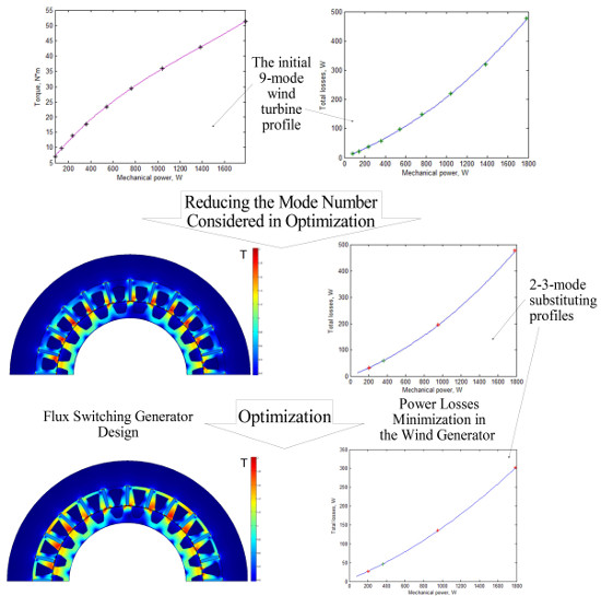
As an example, a gearless FSG was optimized on the basis of the proposed method of constructing the substituting loading profiles for a wind turbine. The wind turbine’s initial profile was specified by nine maximum-power operating points described in [11] over a range of wind speeds. The wind speed was assumed to be distributed according to the Rayleigh distribution. On the basis of the nine-mode profile, two- and three-mode substituting profiles were built. The optimization was carried out with the two-mode profile. The calculations of the initial and optimized designs done with the two-mode and three-mode substituting profiles were compared to the calculations done with the nine-mode profile. It is shown that the results of the calculations done with these three profiles were very close. Some geometrical relations of the optimal FSG were discovered.

2. Short Description of the FSG Design Chosen and Its Mathematical Modeling

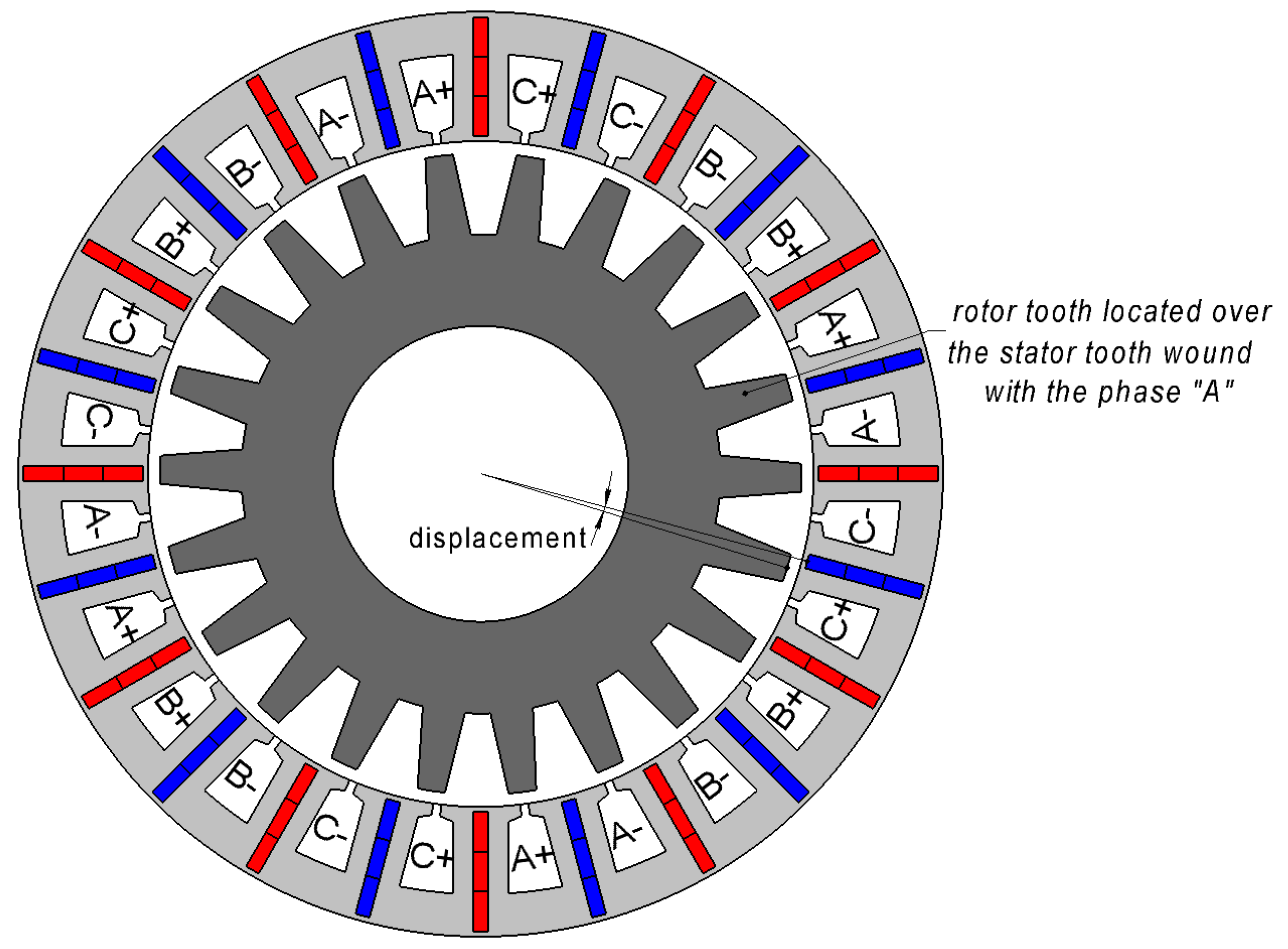
Figure 1 shows a sketch of the FSG design under consideration with 24 stator teeth and 22 rotor teeth. The magnets are inserted in the slits made in each stator tooth. The magnets located in the nearest slits are magnetized oppositely. The stator integrity is provided by thin ribs at the outer and inner stator surfaces. Each second stator tooth is wound. Each magnet is divided into three insulated parts to reduce the eddy currents losses in the magnets.

The mathematical model of an FSG is based on a set of stationary 2D magnetostatic boundary problems for the rotor positions from the interval required by the motor symmetry. The flux linkages, voltages, winding and magnetic core losses, etc., are calculated in postprocessing. The calculation was carried out under the assumption that the phase current was sinusoidal. The motor mechanical power was the model input parameter. The current amplitude had to be determined so as to obtain the required mechanical power [12].

The electric period of an FSG is a rotor rotation by a rotor tooth pitch. Since the rotor had 22 teeth, the electric period was equal to 360/22 = 16.36°. It means that the supply frequency was 22 times higher than that of the rotor rotation (f_e = Z_r × f_m/60, where f_e is the electric supply frequency, Hz; f_m is the mechanical rotational frequency of the rotor, rpm; Z_r = 22 is the number of rotor teeth).

Assume that an FSG rotor tooth is over the middle of the stator tooth wound with the phase ‘A’, as shown in Figure 1. Since the teeth number and the pitches of rotor and stator are approximately equal, and the stator tooth wound with the phase ‘C’ is two stator pitches away, there is a rotor tooth located two rotor pitches away from the first rotor tooth, approximately over the middle of the stator tooth wound with the phase ‘C’. In fact, because of the difference between the rotor and the stator pitches, there is a displacement (Figure 1) between the middles of the rotor tooth and the stator tooth wound with the phase ‘C’ equal to $2\frac{360}{22}-2\frac{360}{24}=\frac{360}{22\times 6}°$ that is equal to one-sixth of the electric period or 60 electric degrees. Therefore, the FSG is symmetrical with respect to the rotation of the rotor by a one-sixth of the electric period and the phase permutation $I_A\to -I_C,I_B\to -I_A,I_C\to -I_B$. Thus, considering the interval of one-sixth of the electric period is enough. In this paper, this interval was divided into 15 equal parts. The number of the boundary problems to solve was 16; 14 of them were inside the interval, and 2 were at its ends.

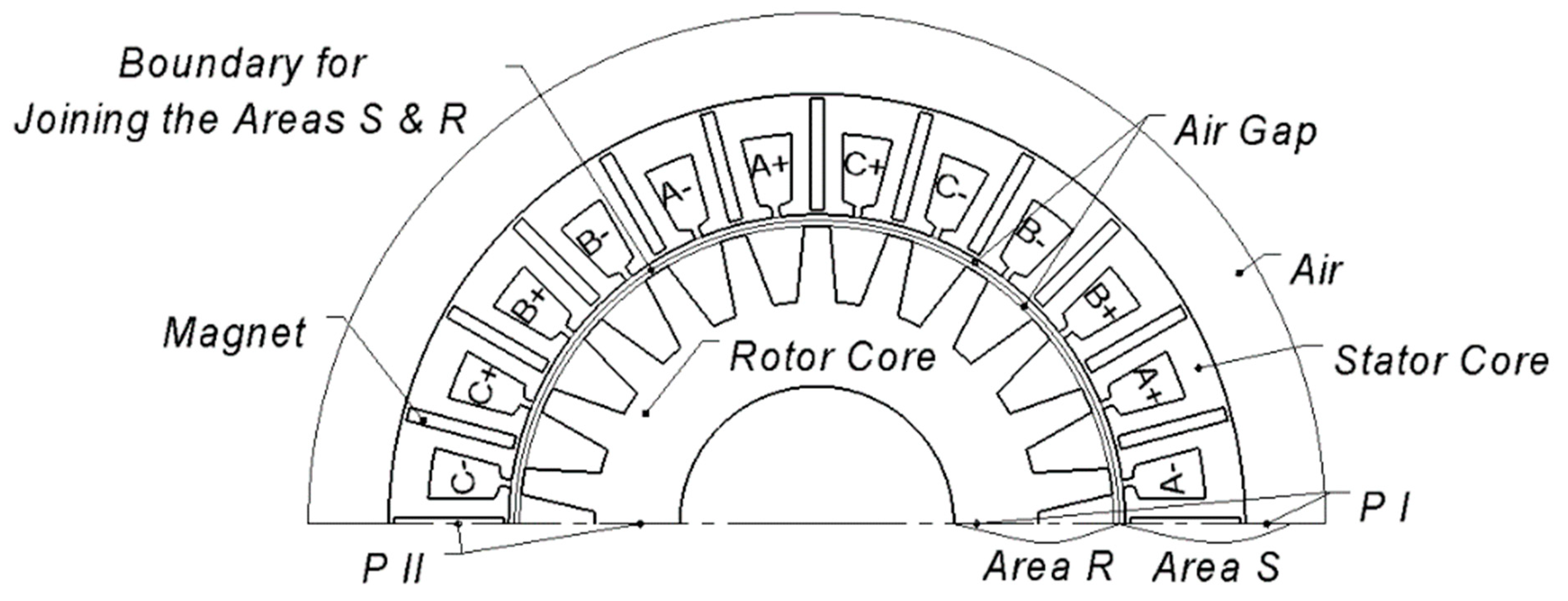
Besides, the flux-switching machine (FSM) symmetry as a whole with respect to a rotation by 180° allowed reducing the calculation area by twice (Figure 2). In this paper, one and the same calculation area was chosen for all boundary problems. The calculation area was divided into two subareas at the middle of the air gap. The rotor position was taken into account by joining these subareas by the boundary condition depending on this angle. Thus, the stator and rotor fields were calculated in their own reference frames. Boundaries P I and P II were joined by the periodic condition [12].

To take into account the magnetic field spread outside the FSM, the air domain whose thickness was equal to the stator tooth pitch, was added beyond the outer stator boundary. Generally, the mathematical model of the FSG was similar to the mathematical models of other machines described in [12,13].

After solving the set of magnetostatic boundary problems, the core and winding losses could be found, as well as the instantaneous fluxes, voltages, torque, etc. In particular, the winding losses were calculated according to Ohm’s law. An instantaneous core losses density is estimated by:

$$p_{st}=\alpha \rho {\left(\frac{dB}{dt}\right)}^2$$

(1)

where ρ is the steel density, and α is the proportionality factor determined on the basis of the empirical data so that p_st, given by the expression (1) and averaged over the electric period, is equal to the reference data for the specific losses in the steel at the supply frequency in the case of sinusoidal flux density and the magnetic flux density of 1 T.

The losses in the magnets were also calculated according to (1). In this case, the expression for α is:

$$\alpha =\frac{{\left(l_{mag}/n\right)}^2{\mu }_0\sigma }{12\rho }$$

(2)

where ${\mu }_0$ is the magnetic constant, $\sigma$ is the specific conductivity of the magnets, $l_{mag}/n$ is the minimal length of the insulated part of the magnets in the direction perpendicular to the flux. If this direction is radial, then $l_{mag}$ is the total length in the radial direction, and n is the number of pieces into which the magnet is divided.

3. Construction of the Generator Substituting Profiles

A load profile of a generator can be described as dependent on the torque T on the shaft, the shaft speed n, and the shaft speed distribution. The load profile can be continuous. Then, the function T(n) and the shaft speed distribution density are to be set. Also, the load profile can be discrete or can be set discretely. Then, the pairs of T and n and the time parts (probabilities) corresponding to those pairs of T and n are to be set.

In the case of wind generators, such profile can correspond to maximum-power operating points.

Setting the load profile allows calculating the average values of the random variables. In particular, in the case of a discrete profile, the average value <A> of any random value A is given by:

$$<A>=\sum p_i{A}_i$$

(3)

where $A_i$ is the value of this variable in the i-th mode, and $p_i$ is the probability of the i-th mode.

The average generator efficiency can be expressed through the average of the mechanical power $P_{mech}=\frac{2\pi nT}{60}$ and the losses power:

$${\eta }_{\mathrm{average}}=1-\frac{<P_{loss}>}{<P_{mech}>}$$

(4)

When the number of the modes is large, the calculation of the averages according to Equation (3) and, in particular, the calculation of the average efficiency according to Equations (3), (4) require large calculation resources. Therefore, an algorithm for constructing the substituting loading profiles containing a lower number of modes is of interest.

Let us consider that the speed n(P_mech) and the torque T(P_mech) of the given profile are functions of the mechanical power P_mech determined on the (continuous) interval of the permissible values of P_mech. When these dependences of n and T on P_mech are set with a table, the values of n and T for an arbitrary value of P_mech are determined by interpolation. As a result, the mode with an arbitrary value of P_mech (but not only with its table values) becomes determined. Therefore, an arbitrarily random value A can be considered as a function of P_mech.

Let the function A(P_mech) on the permissible interval of P_mech be approximated with the polynomial:

$$A=a_0+a_1\times P_{mech}+a_2\times P_{mech}^2+\dots$$

(5)

The operation < > is linear in the following sense:

$$<\alpha x+\beta y>=\alpha <x>+\beta <y>$$

(6)

where $\alpha$ and $\beta$ are numbers, and x and y are random variables. From Equations (5) and (6), it follows:

$$<A>=a_0+a_1<P_{mech}>+a_2<P_{mech}^2>+\dots$$

(7)

So, when the polynomial of the n-th power is sufficient to approximate A, the calculation of its average $<A>$ can be simplified by calculating the same average $<A>$ over the substituting profile whose averages $<P_{mech}>,<P_{mech}^2>\dots <P_{mech}^n>$ coincide with those of the initial profile.

One of the modes which must be considered obligatorily is the rated mode (the mode of the maximum power), because it is needed to calculate the required converter power and to be sure that the magnets are not demagnetized. Setting each underload mode means setting the mechanical power $P_{mech,i}$ and the probability of this mode $p_i$. Therefore, when A can be approximated with a polynomial of 2k-th power, the profile with k underload modes is enough to calculate its average. In particular, the averages $<P_{mech}>$ calculated over the initial profile and any substituting profile having at least one underload mode coincide.

The equations to determine the 2k unknown variables $p_1\dots p_k$, $P_{mech,1}^i\dots P_{mech,k}^i$ are as follows:

$${\displaystyle \sum }_{m=1}^k{p}_m{P}_{mech,m}^i+P_{rated}^i\left(1-{\displaystyle \sum }_{m=1}^k{p}_m\right)=<P_{mech}^i>;i=1\dots 2k$$

(8)

where P_rated is the rated mechanical power.

When quadric approximation is enough, which is in the case of the substituting profile with one underload mode (two-mode profile), there is a simple symbolic solution of Equation (8):

$$P_{mech,1}=\frac{P_{rated}^2-<P_{mech}^2>}{P_{rated}-<P_{mech}>}-P_{rated};$$

(9)

$$p_1=\frac{P_{rated}-<P_{mech}>}{P_{rated}-P_{mech,1}}$$

(10)

In the case of the approximation of the fourth power (three-mode profile), the nonlinear Equation (8) can be solved with any known method, for example, with the Newton’s method.

After finding the mechanical powers in the underload modes of the substituting profile, the speeds and the torques in these modes can be determined by the dependences n(P_mech) and T(P_mech).

4. Example of the Construction of Substituting Two-Mode and Three-Mode Profiles

As an example, the wind turbine described in [11] was considered in this paper. The mentioned study [11] provides the mechanical power and the rotational speed of the turbine in nine maximum operating points corresponding to the wind speeds in the range from 4 to 12 MPS (meter per second). Assume the average speed to be 7 MPS. To approximate the year wind speed distribution, the one-parameter Rayleigh distribution was used [14]. Also, it was accepted in this paper that the wind generator ran only when the wind speed was in the range from 4 to 12 MPS.

To combine the continuous Rayleigh distribution and the nine discrete modes, the Rayleigh distribution was discretized, that is, it was assumed that the wind speed took integer values of MPS. The probability of the integer wind speed is equal to the Rayleigh distribution density. The column p_i in

Table 1. The operating points of the wind generator.

Mode, i	Vi, MPS	ni, rpm	Pmech,i, W	Ti, N∙m	pi
1	4	111	82	7.02	0.134
2	5	140	142	9.69	0.144
3	6	163	237	13.87	0.146
4	7	196	362	17.59	0.138
5	8	221	542	23.41	0.124
6	9	247	761	29.41	0.107
7	10	276	1038	35.88	0.087
8	11	308	1383	42.85	0.069
9	12	332	1784	51.38	0.051

provides the conditional probability when the speed was in the permissible range.

We determined the two-mode and three-mode substituting profiles. The required averages calculated under the initial profile (Table 1) according to Equation (3) are given in

Table 2. The average values of the powers of the mechanical power.

$<{\mathit{P}}_{\mathit{m}\mathit{e}\mathit{c}\mathit{h}}>,\mathbf{W}$	$<{\mathit{P}}_{\mathit{m}\mathit{e}\mathit{c}\mathit{h}}^2>,{\mathbf{W}}^2$	$<{\mathit{P}}_{\mathit{m}\mathit{e}\mathit{c}\mathit{h}}^3>,{\mathbf{W}}^3$	$<{\mathit{P}}_{\mathit{m}\mathit{e}\mathit{c}\mathit{h}}^4>,{\mathbf{W}}^4$
541.9	5.177 × 105	6.472 × 108	9.228 × 1011

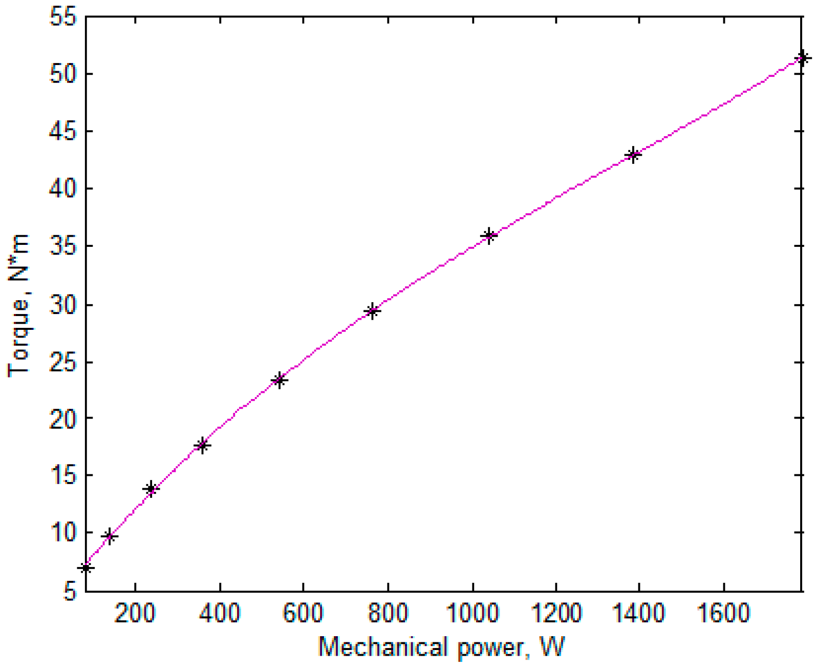
. The mechanical powers in the underload modes and their probabilities were determoned by Equations (8), (9), (10). Figure 3 shows the torques and the mechanical powers at nine modes in the initial profile, with ‘*’ as well as the cubic polynomial approximating this dependence. Then, the torques of the substituting profiles were determined using this approximation. After that, the rotation speeds were calculated (

Table 3. The two-mode substituting profile.

Mode, i	ni, rpm	Pmech,i, W	Ti, N∙m	pi
1	193.6	361.6	17.84	0.873
2	331.6	1784.3	51.38	0.127

and

Table 4. The tree-mode substituting profile.

Mode, i	ni, rpm	Pmech,i, W	Ti, N∙m	pi
1	161	206.3	12.24	0.623
2	268.1	952.3	33.92	0.311
3	331.6	1784.3	51.38	0.066

).

Table 3 shows the two-mode profile, and Table 4 shows the three-mode profile.

5. Optimization Routine

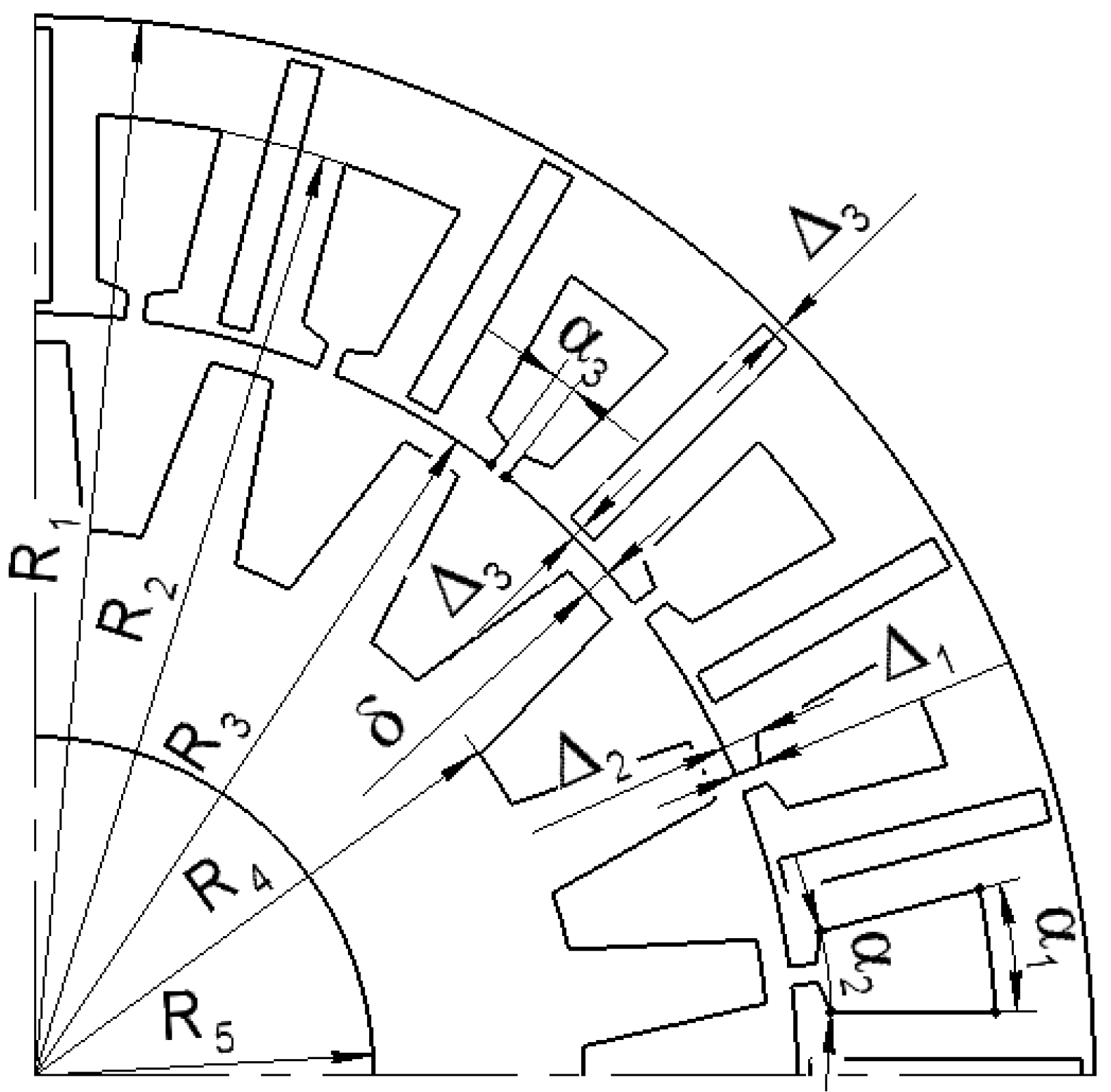
Figure 4 shows the main geometric dimensions of the FSG. The FSG parameters fixed during the optimization are given in

Table 5. The fixed FSG parameters during the optimization.

Parameter	Value
Outer radius of the stator ($R_1$), mm	80
Air gap ($\delta )$, μm	350
Rotor slot depth ($R_3-\delta -R_4$), mm	9
Rotor yoke thickness ($R_4-R_5$), mm	5
Stator ribs thickness ${\mathsf{\Delta }}_3$, μm	500
Remanent flux density of the magnets, T	1.2
Angular size of the stator slot opening (α3), ts	0.162
Rotor and stator cores length (L), mm	100

. The angular dimensions of the stator are given in the stator tooth pitch, $t_s=\frac{360}{24}=15°$, and those of the rotor are given in the rotor tooth pitch, $t_r=\frac{360}{24}=16.36°$. The parameters that varied during the optimization are given in

Table 6. The varied FSG parameters during the optimization.

Parameter	Value
Radius of the stator slot bottom ($R_2$), mm	74
Inner stator radius ($R_3$), mm	61.7
Angular size of the stator slot α1, ts	0.45
Angular size of the stator slot α2, ts	0.5
Magnets thickness, mm	2
Angular size of the rotor tooth surface facing the air gap, tr	0.265
Current angle in the rated mode, el. Radians	0.1

. To reduce the reactive power, the field-weakening technique was applied. The current angle was assumed to be proportional to the torque; the zero angle of the current was chosen when there was no field weakening.

A multi-objective optimization most fully meets the requirement of designing an electrical machine for a real application [15]. Some multi-objective methods are aimed at building the Pareto front, which is the set of the solutions in which no objective can be improved without worsening other objectives. In this case, the engineer chooses the solution in the Pareto front in which the objectives reach their values according to their importance in the given task.

Another approach to multi-objective optimization is implemented on the basis of the methods of optimization with one criterion. In this case, the importance of the objectives should be set by constructing the optimization criterion as a function of these objectives. It is possible to use both encouraging and fining components of this function [16].

So, for any multi-objective optimization to be implemented, the importance of the objectives must be set either at the optimization beginning or at its end.

In this paper, the selection of the optimization algorithm was influenced by the smoothness of the objective function and the presence of computational errors that arose because of the finite number of considered boundary value problems with different positions of the rotor and finite size of the mesh elements. These factors create a pseudo-random error that is difficult to predict. Therefore, the objective function calculated using the finite element method (FEM) is noisy, and the gradient methods usually used for smooth functions with a low number of extrema cannot be applied [12,13].

To overcome these difficulties, the gradient-free method known as the Nelder–Mead method [17] was used in this work. This method is based upon the comparison of the criterion values for various solutions, but not upon their numerical values. Therefore, it can be used for noisy or non-smooth functions. Moreover, it can be more effective than some other gradient-free methods, in particular, the Powell method [12,18].

The objective function used was as follows:

$$F=K_1{K}_2^2{K}_3^{0.5},$$

(11)

where K₁, K₂, and K₃ are the optimization objectives, namely, $K_1=<P_{loss}>$ is aimed to increase the generator efficiency and AEP, and K₂ is the required frequency converter power

$$K_2=3\frac{I_{ampl,rated}}{\sqrt{2}}\frac{U_{DC,rated}}{\sqrt{6}},$$

(12)

where I_ampl,rated and U_DC,rated are the current amplitude and the DC voltage of the frequency converter required at the rated conditions (T = 100%, n = 100%), that is, when these parameters reach their maximum values. The parameter K₂ coincides with the apparent power when the current and the voltage are sinusoidal and symmetric and is expressed through U_DC,rated, which is the converter limitation. $K_3=L(h_{mag}+0.001\mathrm{m})l_{mag}$, where $l_{mag}=R_1-R_3-2{\mathsf{\Delta }}_3$ is the radial length of the magnets, is to decrease the cost of the magnets and similar to the volume, i.e., equal to the product of three dimensions of the magnets, of which the magnet thickness is increased by 0.001 m to take into account that thin magnets cost more than thick ones [19].

Equation (11) determines the merits of the objectives and means that decreasing $K_1$ by 1%, decreasing $K_2$ by 0.5%, and decreasing $K_3$ by 2% are equally valuable. If an engineer is not satisfied with the optimization results, a new optimization with new merits can be started from the optimized solution. The higher the exponent of the objective, the more valuable the objective is.

6. Investigating the Initial Design

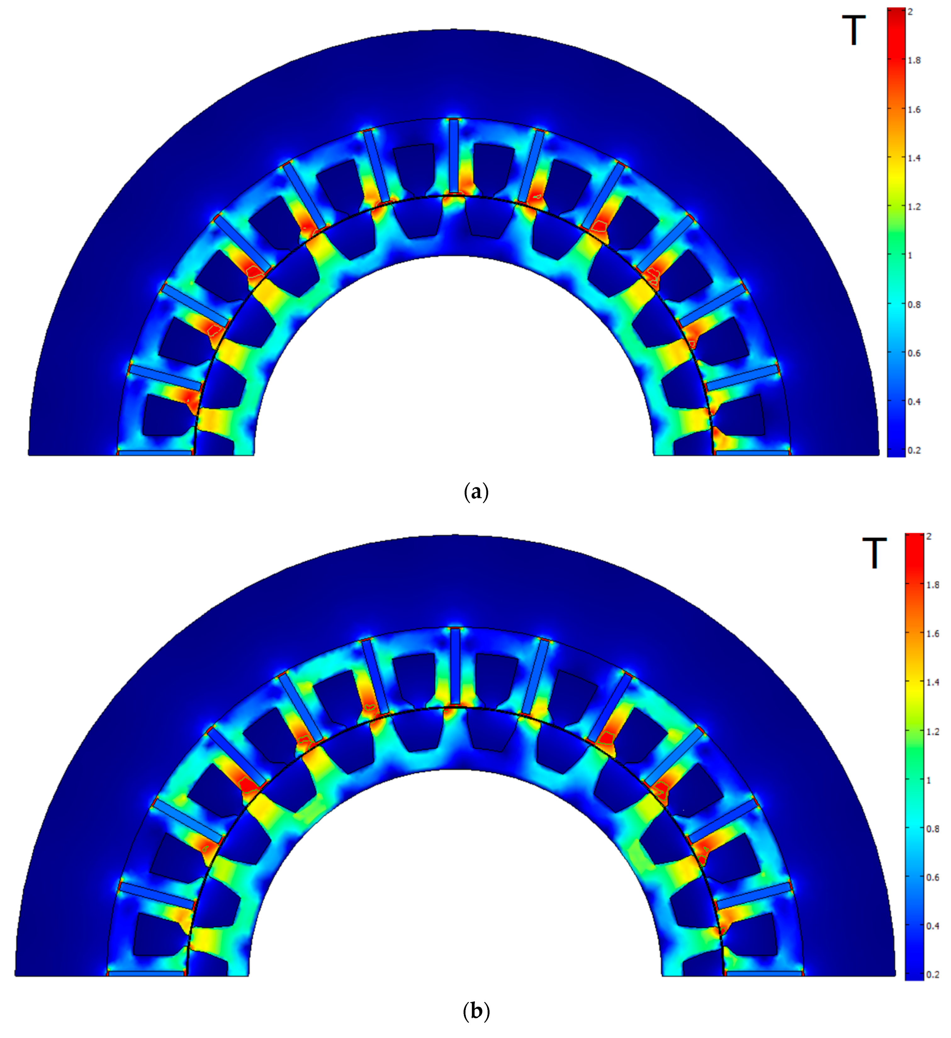
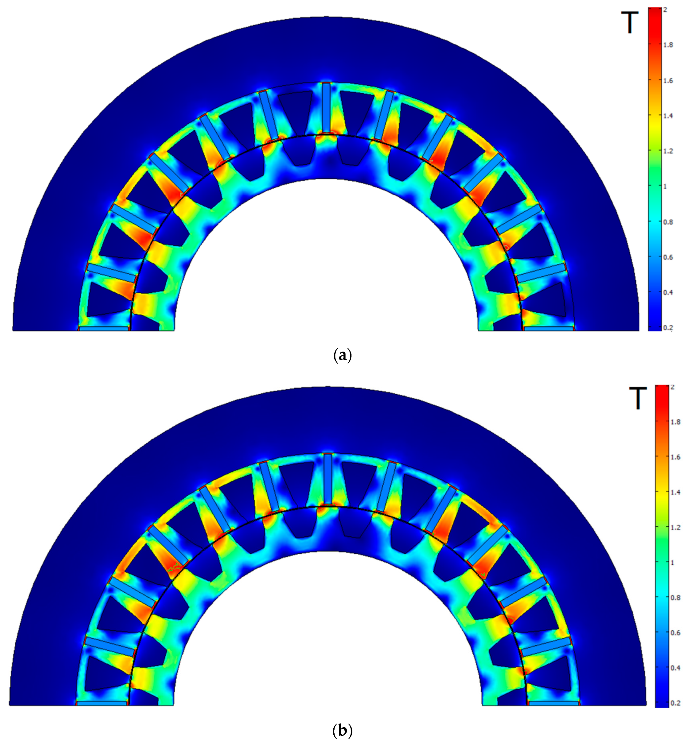
Figure 5 shows the magnetic flux density of the FSG at the rated torque and at the underload mode of the two-mode profile. Because of the effect of the flux concentration, the magnetic flux density reached the value of 1.95 T not only in the ribs but also in some stator teeth. Thin green isolines of 1.85 T were added to the picture to show the areas of extreme saturation. The large volume of the extreme stator tooth saturation impeded the flux flow. So, the problem of calculating FSM was extremely nonlinear, and the possibility of approximating the losses with low-power polynomials was not obvious.

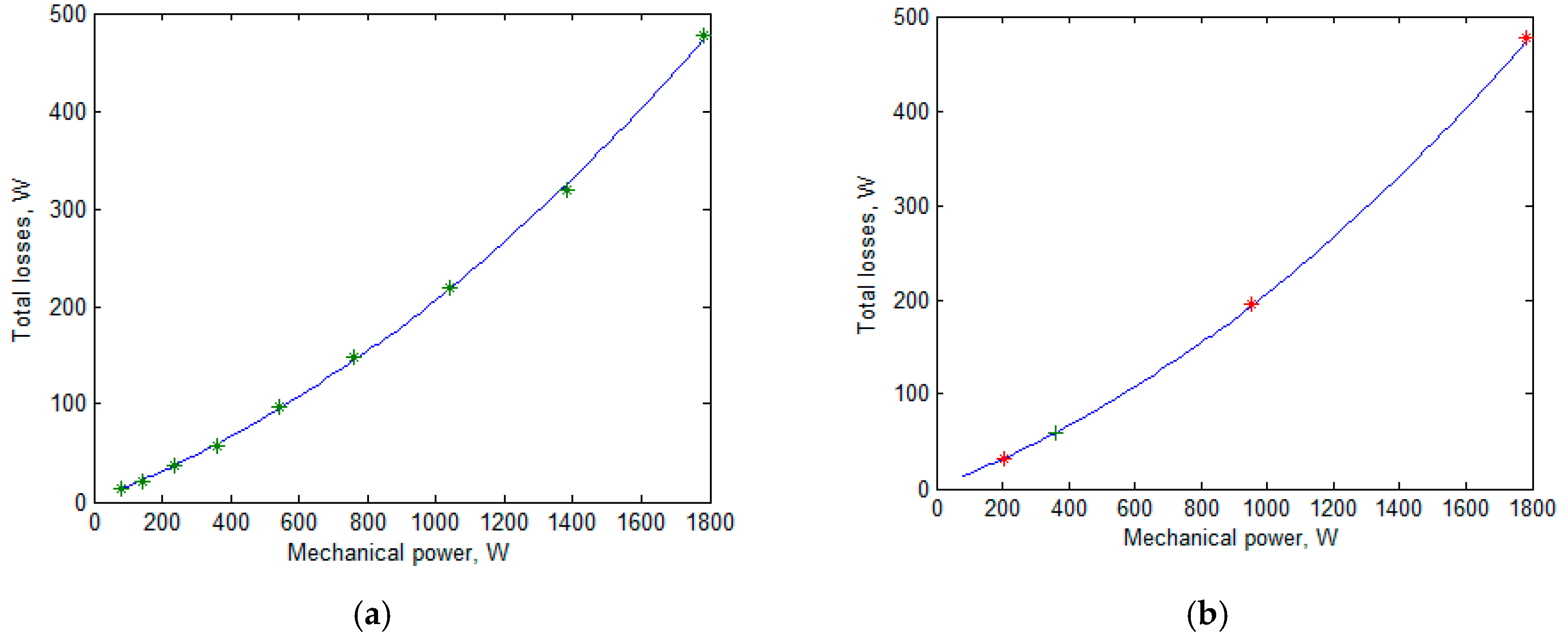
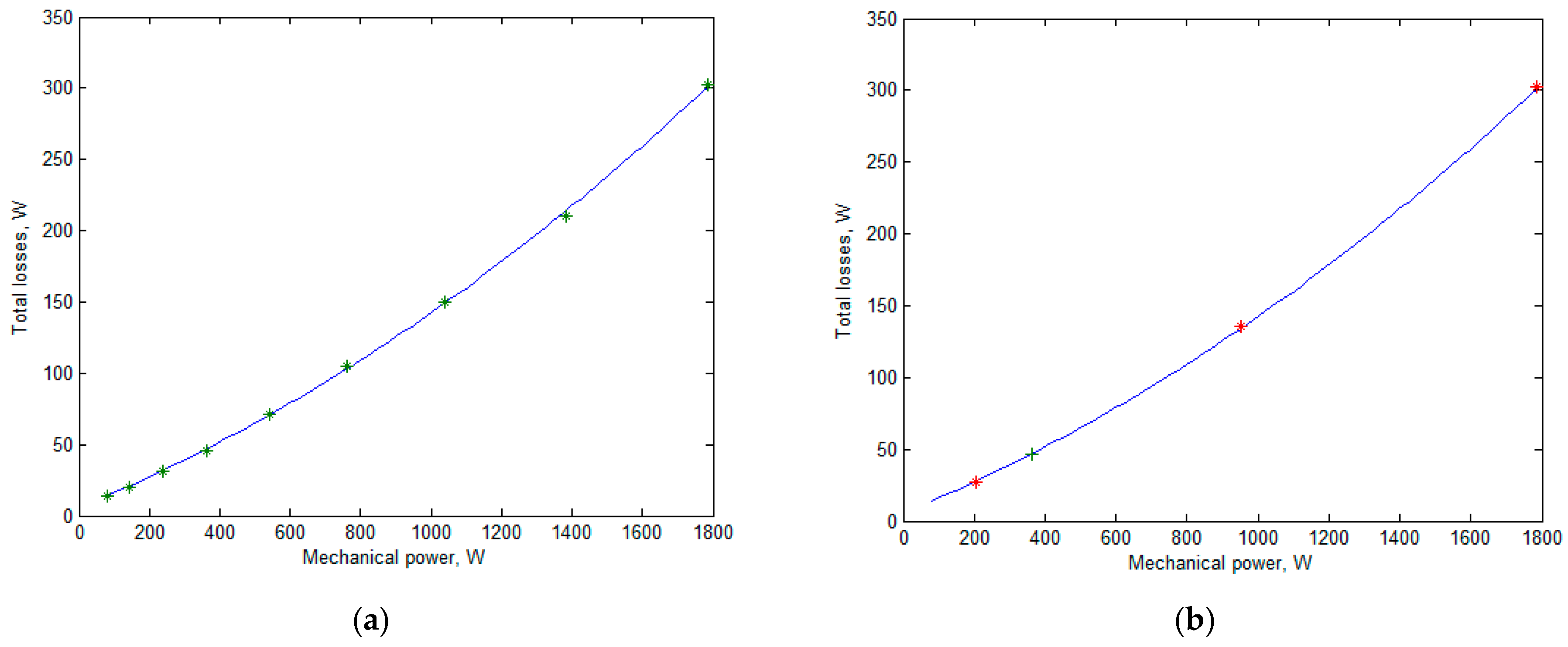
The FSG losses for the two-, three-, and nine-mode profiles are given in

Table 7. The calculated losses of the initial FSG design.

Mode	Losses, W
	2-Mode Profile	3-Mode Profile	9-Mode Profile
1	58.9	31.4	13.3
2	476.6	196.5	21.7
3	-	476.6	37.8
4	-	-	57.8
5	-	-	96.1
6	-	-	148.1
7	-	-	220.1
8	-	-	319.3
9	-	-	476.6
average	112	112.1	112

. The mechanical losses were assumed to be equal to $3\left[W\right]\left(\frac{n}{n_{rated}}+{\left(\frac{n}{n_{rated}}\right)}^3\right)$. The average losses for the two- and nine-mode profiles almost coincided (the difference was less than 0.03 W). The average losses for the three-mode profile differed from the previous ones by 0.1 W. To be sure that the coincidence of the numeric values of the losses was not accidental, the nine modes of the nine-mode profile are shown with ‘*’ in Figure 6a; the quadric trinomial approximating these modes is also shown. The same parabola is shown in Figure 6b. Also, the modes of the three-mode profile are shown with ‘*’, and the underload mode of the two-mode profile is shown with ‘+’. The figures show that all these modes were approximated well with the parabola. Therefore, the approximation was carried out under the two-mode profile in this work.

7. Optimization and Results

In this paper, the optimization was carried out according to the criterion (11) for the two-mode substituting profile. The calculation of the objective function required twice as much calculation efforts as in the case of the optimization based only on the rated mode calculation. However, the proposed approach was aimed to increase the average efficiency over the wide range of speeds and powers. Compared to using the average efficiency over the nine modes, the computational efforts for one calculation of the objective function were reduced by 4.5 times.

Figure 7 shows the geometry of the FSG optimized design and the magnetic flux density at the rated mode and at the underload mode of the two-mode profile. Thin green isolines of 1.85 T were added to the picture to show the areas of extreme saturation. Compared to Figure 5, the magnetic flux density did not reach 1.95 T, except for the stator ribs. Also, the volume of the extreme saturation of the stator core was significantly diminished during the optimization. The yoke thickness R₁ − R₂ was reduced. The stator teeth thickness narrowed at the base and thickened near the air gap.

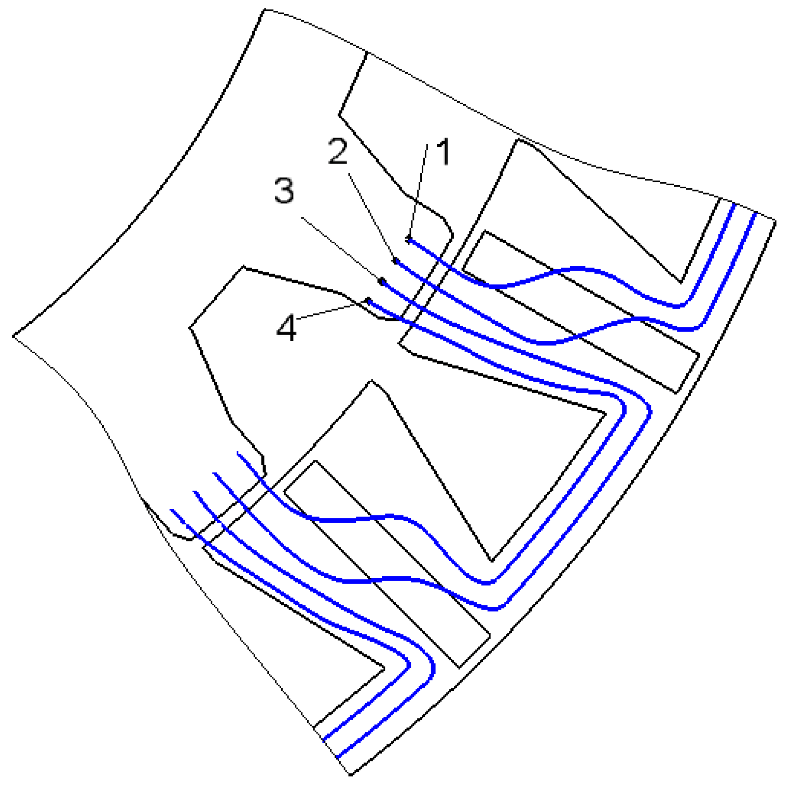
Figure 8 clarifies such pattern. When the rotor tooth is over the half of the stator tooth, the magnetic flux flowing into this half and shown with the magnetic field lines 1, 2, 3, 4 closes through the yokes and splits into two fluxes, i.e., 1, 2 and 3, 4. To conduct such fluxes, a yoke thickness approximately equal to the half of the half of the stator tooth is enough. Besides, the flux 1, 2 crosses the magnet to another part of the stator tooth uniformly and almost weakens fully at the stator tooth base. Therefore, the thickness of the half of the stator tooth at its base is approximately equal to the yoke thickness. These geometric ratios can be slightly broken in the optimal design of an FSM with rare-earth magnets. However, they can be used to get a good initial design for optimization.

As it has been mentioned above, the dependence of the losses on the mechanical power for the initial design can be described well with a square trinomial. To be sure that this is true also for the optimal design, the calculations of the optimized FSM under the three-mode and nine-mode profiles were performed.

The losses in the various modes are given in

Table 8. The calculated losses of the optimized FSG design.

Mode	Losses, W
	2-Mode Profile	3-Mode Profile	9-Mode Profile
1	46.5	27.6	13.6
2	302.2	135.1	20.4
3	-	302.2	31.7
4	-	-	46
5	-	-	71.1
6	-	-	104.5
7	-	-	149.9
8	-	-	210.8
9	-	-	302.2
average	79	79.2	78.8

. Although the differences between the results of the calculations of the average losses under the two-, three-, and nine-mode profiles for the optimized design were higher than those for the initial design, the results of these calculations were similar. Figure 9 is similar to Figure 6 and demonstrates that the dependence of the losses on the mechanical power for the optimized design could be accurately approximated with a quadric trinomial, which confirmed the correctness of the optimization with the two-mode profile.

The main parameters of the FSG before and after the optimization are given in

Table 9. The main parameters of the FSG before and after optimization.

Parameter	Value
	Initial Design	Optimized Design
Radius of the stator slot bottom ($R_2$), mm	74	77.2
Inner stator radius ($R_3$), mm	61.7	63.3
Angular size of the stator slot α1, ts	0.45	0.28
Angular size of the stator slot α2, ts	0.5	0.558
Magnet thickness, mm	2	2.41
Angular size of the rotor tooth facing the air gap, tr	0.265	0.324
Current angle in the rated mode, el. Radians	0.1	0.086
Average losses, $K_1$, W	112	78.8
Average efficiency under the nine-mode profile, %	79.4	85.5
Required converter power ($K_2$), W	1973	1767
$K_3=L(h_{mag}+0.001 \mathrm{m})\left(R_1-R_3\right)$, m3	5.478 × 10−6	5.71 × 10−6
Torque ripple at the rated mode, %	1.6	1.3
Cogging torque, N∙m	0.6	0.43
Mass of the magnets, kg	0.613	0.674
Mass of the copper, kg	1	1.06
Mass of the stator core, kg	3.88	3.26
Mass of the rotor core, kg	2.17	2.46
Objective function (F), W3m3/2	1881	1087
Active material mass, kg	7.66	7.45

.

8. Conclusions

This paper describes the optimization procedure of a gearless FSG for a wind turbine. The average losses over the wind turbine profile, the required converter power, and the parameter $K_3$ representing the cost of the magnets were chosen as the optimization objectives. $K_3$ was developed so as to take into account the fact that thin magnets are more expensive than thick ones.

A detailed wind turbine profile contains a large number of modes. In this paper, the nine-mode profile presented in a previous study [11] was considered. To reduce the calculation efforts during the optimization, we proposed a method for constructing the substituting profiles. Two-mode and three-mode substituting profiles were constructed on the basis of the nine-mode initial profile. The average losses, calculated for the two-mode, three-mode, and nine-mode profiles, accurately coincided, which supports the use of the low-mode substituting profiles instead of the initial profile.

Therefore, the optimization was carried out on the basis of the two-mode substituting profile. The calculation of the objective function requires twice as much calculation efforts with respect to the optimization based on the rated mode calculation only. However, the proposed approach is aimed at increasing the average efficiency over the wide range of speeds and powers. Compared to using the average efficiency over the nine modes, the computational efforts for one calculation of the objective function were reduced by 4.5 times.

Since the multi-objective optimization is a compromise between objectives, a decrease in one objective, may result in an increase in other objectives. During the optimization, the average losses decreased by 30%, which corresponded to an increase in the average efficiency by almost 6%, and the required converter power decreased by 10%. However, thei required an increase in the objective $K_3$ by 4% and an increase in the mass of the magnets by 10%. Such increases had little influence on the cost of the wind turbine as a whole, including tower, blades, electronics, battery, etc. The total active material mass decreased. Also, a decrease in the cogging torque and in the torque ripple was found.

Some preferable geometric features of FSG were found out thanks to this optimization, among which the trapezoidal form of the stator teeth, thinning near its base.

In the future, a prototype will be manufactured, and its experimental verification will be performed. Also, the FSG will be compared with a surface-mounted permanent magnet synchronous motor.