Article

Short-Term Load Forecasting for a Single Household Based on Convolution Neural Networks Using Data Augmentation

1
Department of Electronics Engineering, Mokpo National University, Muan 58554, Korea
2
School of Electrical and Electronic Engineering, Gwangju University, Gwangju 61743, Korea
3
Department of Information and Electronics Engineering, Mokpo National University, Muan 58554, Korea
*
Author to whom correspondence should be addressed.
Energies 2019, 12(18), 3560; https://doi.org/10.3390/en12183560
Submission received: 16 August 2019 / Revised: 11 September 2019 / Accepted: 15 September 2019 / Published: 17 September 2019
(This article belongs to the Special Issue Short-Term Load Forecasting 2019)

Abstract

:
Advanced metering infrastructure (AMI) is spreading to households in some countries, and could be a source for forecasting the residential electric demand. However, load forecasting of a single household is still a fairly challenging topic because of the high volatility and uncertainty of the electric demand of households. Moreover, there is a limitation in the use of historical load data because of a change in house ownership, change in lifestyle, integration of new electric devices, and so on. The paper proposes a novel method to forecast the electricity loads of single residential households. The proposed forecasting method is based on convolution neural networks (CNNs) combined with a data-augmentation technique, which can artificially enlarge the training data. This method can address issues caused by a lack of historical data and improve the accuracy of residential load forecasting. Simulation results illustrate the validation and efficacy of the proposed method.

1. Introduction

Short-term load forecasting (STLF) is an important part of power system planning and operation [1]. The STLF, which has a prediction range of one hour to 168 h, is used for controlling and scheduling of daily power system operations. Furthermore, forecasting customer-level energy consumption is essential for many potential applications in the future power system, such as demand response (DR) programs, home load scheduling with renewables, and optimal operation of energy storage systems (ESS) [2].
Statistical methods, including multiple linear regression [3,4], exponential smoothing [5], and the autoregressive integrated moving average (ARIMA) [6] are the most commonly used for the STLF. Recently, deep-learning-based forecasting techniques are gaining attention in the STLF. Recursive neural networks (RNNs) capable of learning long-term dependence are being applied to the assumption of load prediction in [7]. However, the vanishing gradient problem of RNNs makes it hard to improve forecasting accuracy. In [8,9], to overcome this problem in the RNN, the long short-term memory (LSTM) has been proposed. Some studies show the capability of LSTM for more improved forecasting performance at the system-level forecast when there is relatively long-term historical load data. In addition to the above methods, many deep learning algorithms, such as deep feed forward [10,11], deep belief network (DBN) [12], are being applied to load forecasting. In addition, some hybrid spectral methods, including wavelet analysis [13] and empirical mode decomposition (EMD) [14] with neural networks, have been proposed to remove the uncertainty of historical electrical load. However, all of these techniques were implemented in the substation- or system-level load forecasting with training from sufficient historical load data.
In the STLF at the system-level, a lot of historical data are available because small electrical load changes do not significantly affect the overall load pattern trend. However, at the household level, STLF may not have enough data for some households to capture long-term dependencies and properly train the learning network. For example, if a homeowner has recently changed, only a small amount of electrical load data will help its load forecasting. In addition, even if homeowners have not changed for a long time, the pattern of energy consumption can change with new electrical devices and lifestyle changes [15]. Therefore, there is a limit to using the previous data to increase the training data size. In [2,7], RNN and LSTM were applied to single household load prediction, but these studies did not take into account the past data shortage issues.
To address the lack of historical data for training, the convolutional neural networks (CNNs) can be an effective method for residential load forecasting, because CNN can capture short-term trends in load data when the local data points are strongly related to each other [16]. In addition, data augmentation can be one solution to handle the issues. Data augmentation can handle short-duration data collection by enlarging the size of the training data in a way that adds extras copies of training examples in training dataset and minimizes the overfitting in deep-learning techniques [17]. The overall training cost of a deep network will be reduced when input data are large and contain more similar information. With such enlarged training data, the accuracy of residential load forecasting can be improved. Technical paper [7] tries to enlarge the input data using another household’s load series. However, this approach has the potential to obtain data that have different characteristics of the load series of the target household. Moreover, some target households have similar load profiles in their load series, but others do not [2]. Because of load profile diversity within and between households, existing forecasting benchmarks yield cons rather than pros. In fact, forecasting with only a single household’s data may not often have sufficient information to fit a wide variety of the model capacity, particularly in deep-learning techniques. Therefore, proper data augmentation is required, which can artificially create new training data from the historical data of a single household.
Herein, the paper proposes a load-forecasting method for a single residential household based on convolutional neural networks (CNNs). The CNN is a type of deep neural network where its structure is formed by using convolution and pooling layers [18,19,20]. With the help of various filters, CNNs can learn the inherent information of an electric load series. The proposed forecasting introduces a novel data augmentation technique that concatenates the various residual load series generated from the electrical load of a single household. The original load series is converted to another residual load series containing uncertainty information of electrical load. Several residual load series are extracted through multiple k-means clustering to collect sufficient training data [21,22]. Among the extracted residual load series, the less uncertain and more homogeneous ones were fed to the CNNs as training data. The proposed augmentation technique can provide enough homogeneous training data to CNNs for more accurate forecasting. The proposed forecasting method was tested on ten single households for a year and is compared with the results of pooling-based augmentation [7].
The rest of this paper is organized as follows. Section 2 discusses the implementation of the proposed augmentation strategies and the context of residual load series. Similarly, Section 3 describes the proposed algorithm. Section 4 talks about the implementation procedure and discusses the simulation results. Section 5 concludes the paper.

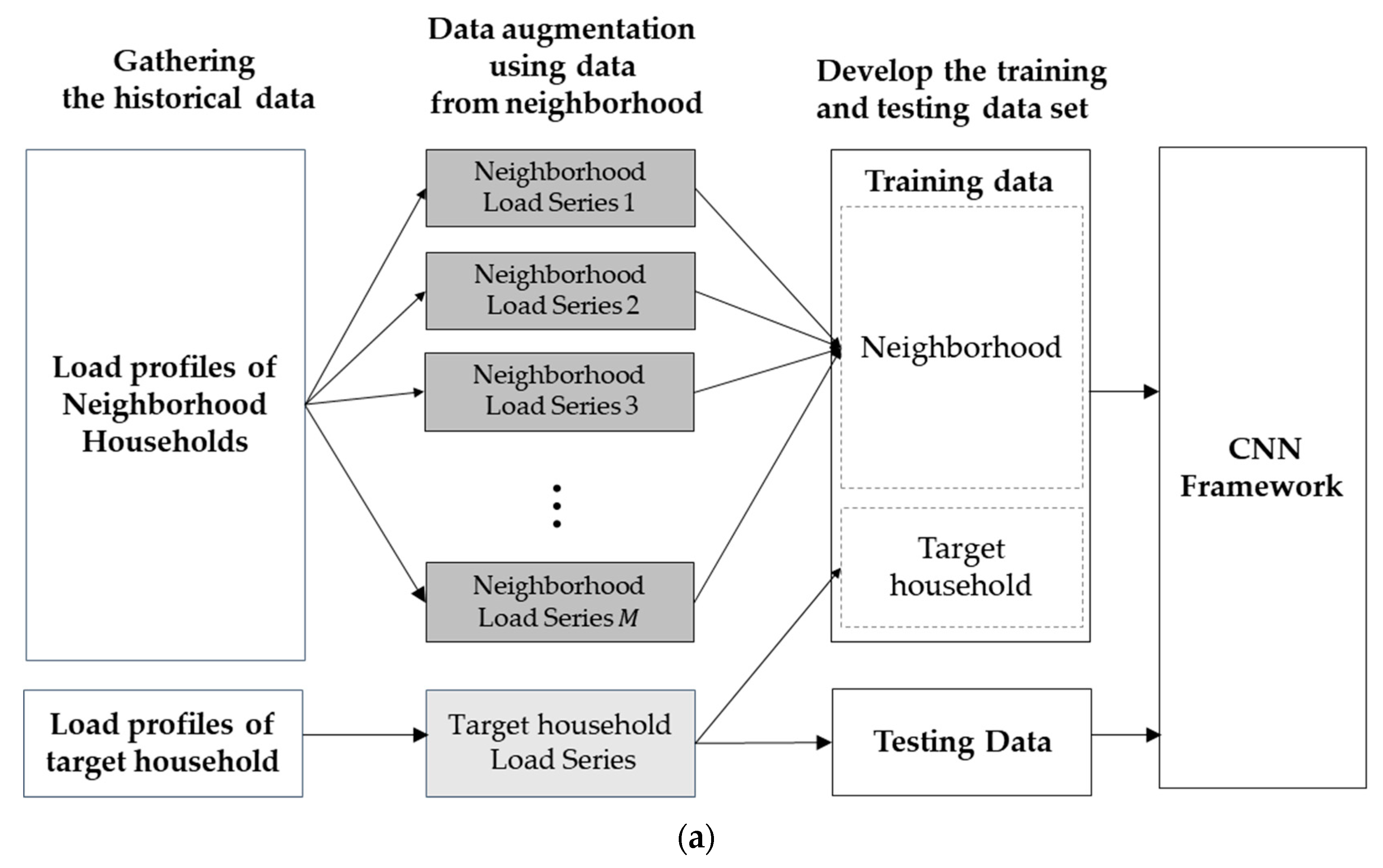
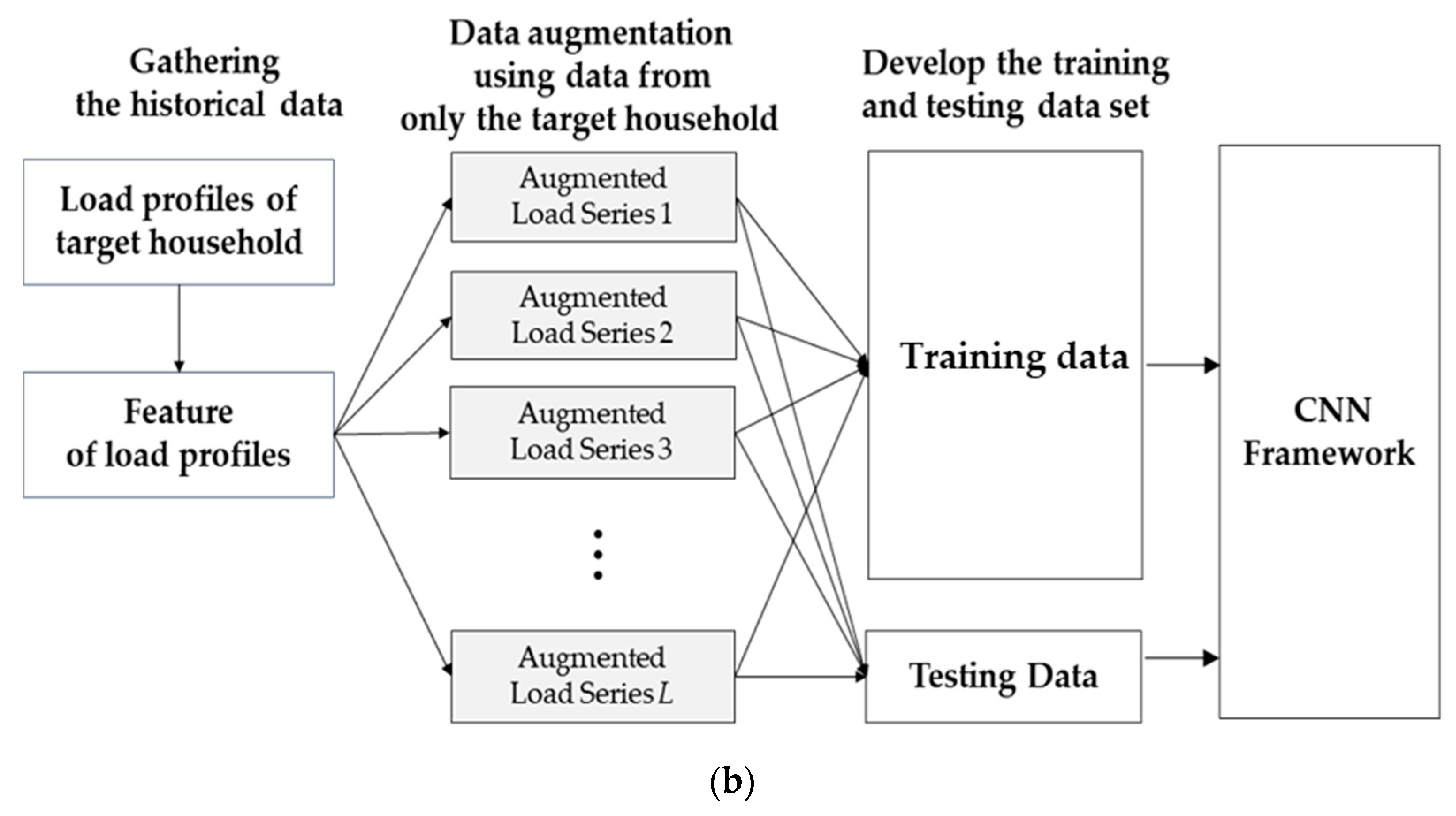
2. Augmentation Implementation

2.1. CNN with Augmentation

Since an electric load series consists of many load profiles, the diversities between the load profiles are a major concern for forecasting using CNN filter networks. In fact, CNNs can facilitate more precisely given less diverse training load profiles rather than highly diverse ones [23]. Because of human actions, weather, and types of day, the differences between load profiles are uncertain, non-linear, and complex [2,24]. On the other hand, the amount of training data is crucial for fitting all the parameters of CNNs.
To address the issues of the uncertainty and necessities of huge training data, the state-of-the-art papers used other households load series for data augmentation. Moreover, the existing approaches do forecasting by hoping that load profiles will repeat and assume that the repetition of load profiles is often similar among households during the same time interval [7,23]. As a consequence, the forecasting accuracy is trivialized when the augmented data contains only correlated households’ load series. However, the effects of human actions and the type of day are totally different in the electricity load of a single household and are too difficult to predict. Thus, incorporating other households’ load series into training data inevitably burdens the learning ability of the CNN rather than optimizing it.
The augmentation strategy can be applied with single households and is valid when each deep-learning-based forecasting framework improved its performance [25,26]. To improve cognition, augmentation techniques need to grasp all the potentially uncertain information about the electric load series. Figure 1a,b describe the concept of enlarging data with the existing pooling and proposed augmentation approach for deep-learning-based forecasting. To enlarge data, the proposed method artificially generates several augmented load series, each of which needs to be extracted in a way that facilitates the CNN learning strategies. To obtain a rationale, each series should have less uncertain and more homogeneous information. The appropriate series are concatenated with each other to turn out a huge amount of training data with homogeneous information. The more homogeneous information there is, the more useful it is for a CNN network to address the granular-level load prediction. Any dissimilar augmented load series in concatenation could destroy a CNN’s optimal cognition. The procedure of extracting a homogeneous information load series is vital and depends totally upon imagination [27]. The proposed augmentation strategies are described in the following section.

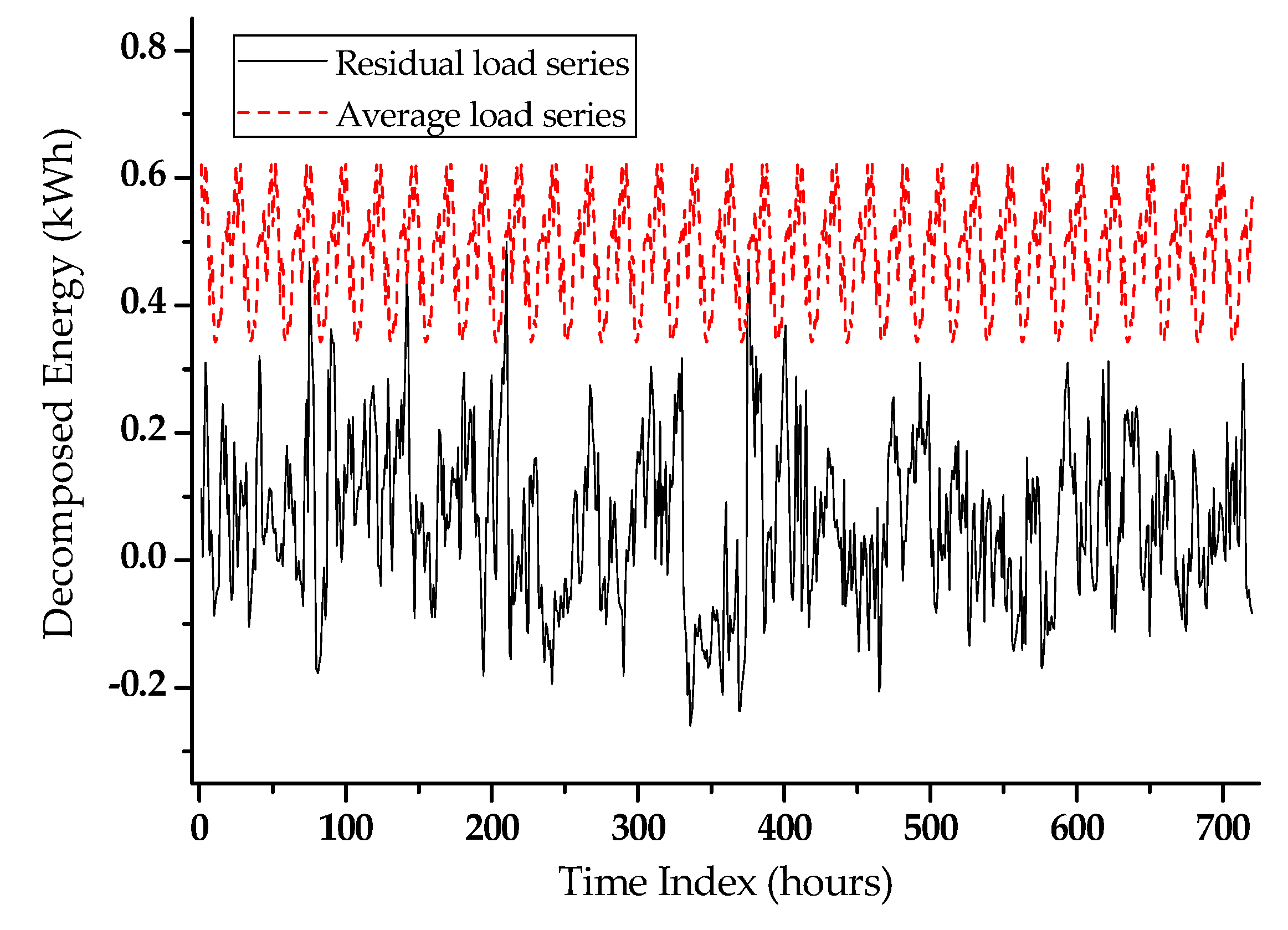
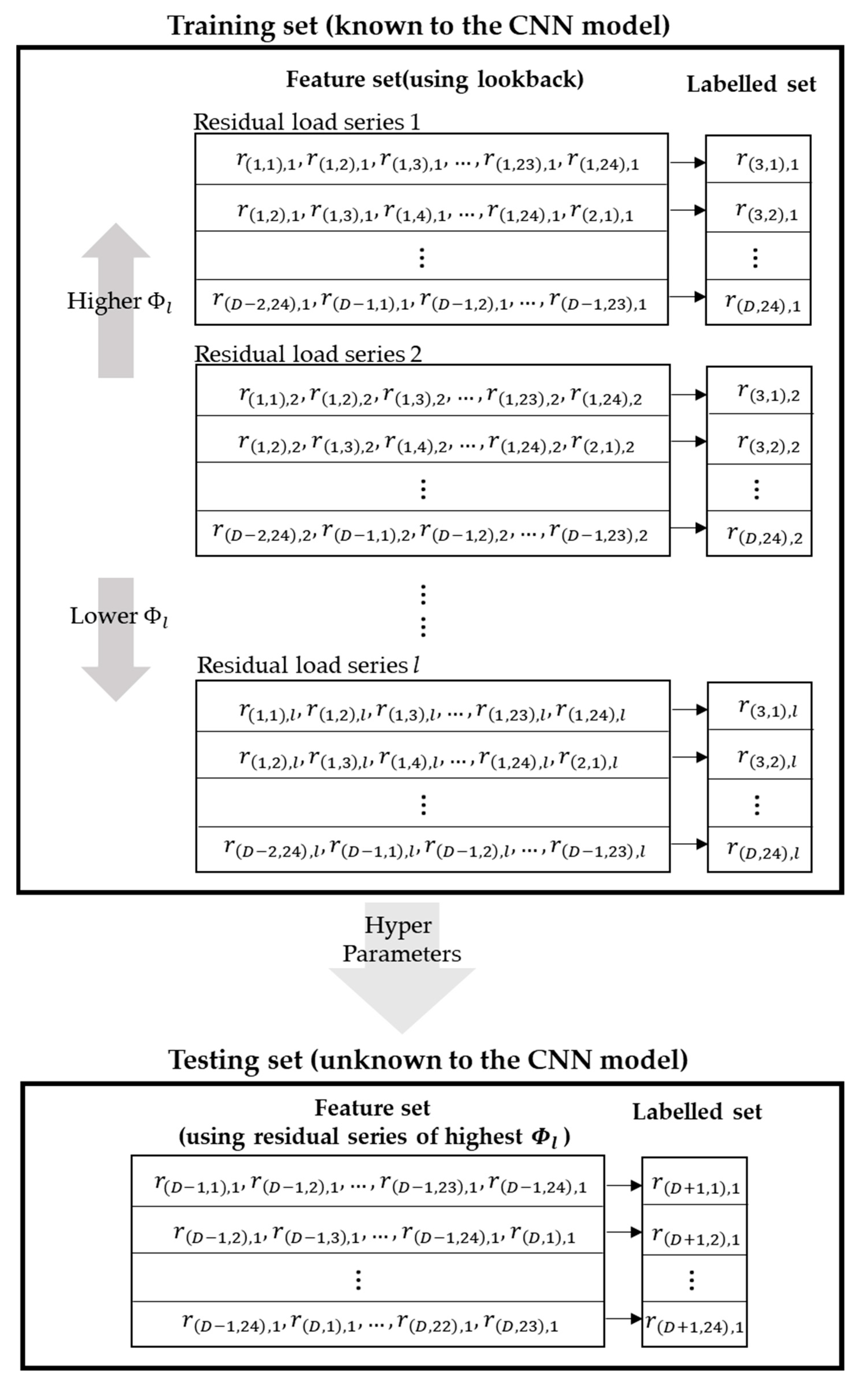
2.2. Extraction of Residual Load Series

The data structure of the historical electricity load of a target household can be expressed as the following matrix:
P = [ p 1 , 1 ,   p 2 , 1 ,   , p 1 , t , , p 1 , T p 2 , 1 ,   p 2 , 2 ,   , p 2 , t , ,   p 2 , T p d , 1 ,   p d , 2 ,   , p d , t , , p d , T p D , 1 ,   p D , 2 ,   , p D , t , , p D , T ] ,
where p d , t represents historical electric load at time t in day d; D represents the number of days of historical data, and the time period T is 24 h. This matrix of a historical load can be simplified as follows:
P = [ p 1 ,   p 2 ,   p 3 , , p d , , p D ] ,
where vector p d are the hourly load profiles of a target household in day d. Figure 2 shows all daily load profiles of a household for one month. In Figure 2, it can be found that the electrical load of a single household fluctuates abruptly. Generally, a smaller electricity load tends to have a higher variation, which makes it difficult to accurately forecast the residential electricity load. In CNN-based forecasting, one way to achieve high performance is to reduce the variations of training data [21].
To improve the learning ability of CNNs, one must extract new features from a residential load series, which has less volatility but still has inherent characteristics of a residential load. One way to reduce the variation is to remove the regular pattern from the load series [28] so that CNNs use only its residuals. With this approach, each load profile is decomposed into centroid and residual load profiles as follows:
p d = c + r d   ,
where vector c is the centroid load profile (average profile) of the historical load, and r d is a vector of the residual load series which is the difference between a given centroid c and an actual load profile on day d . The centroid load profile can be used as the baseline of a particular group of daily load profiles, and the repetition of the centroid load profile yields an average load series for a certain duration. Figure 3 shows an average load series, and its residual load series of a residential household for a month. In Figure 3, the average load series does not contain any uncertain information, but it shows only a regular pattern. On the other hand, the residual load series contains all the uncertain and complex information about the residential load. The residual load series is less volatile than is the original load series but still has inherent characteristics of the residential load. With training from this less volatile data, the CNNs can forecast the small residential load more accurately.
To ensure the appropriateness of the residual load series in learning networks, auto-correlation (AC) or partial auto-correlation (PAC) coefficients [29] can be used. Higher AC or PAC coefficients, out of the confidence interval, mean that the present residual load series is strongly coupled with the historical residual load series. Figure 4 shows AC and PAC coefficients of the residual load series of a selected single household with different time lagging. As shown in Figure 4, when the lags are the multiple of 24 h, the AC coefficients would peak, so that some AC coefficients are out of the confidence interval. Similarly, the PAC coefficient spikes also confirm that the residual load series has vital information about the residential electricity load. The information is in a hidden state and can be learned by using learning networks.
With these residential load series, the paper proposes a CNN-based method for residential load forecasting using data augmentation. The augmentation technique and overall forecasting procedure are described in the following section.

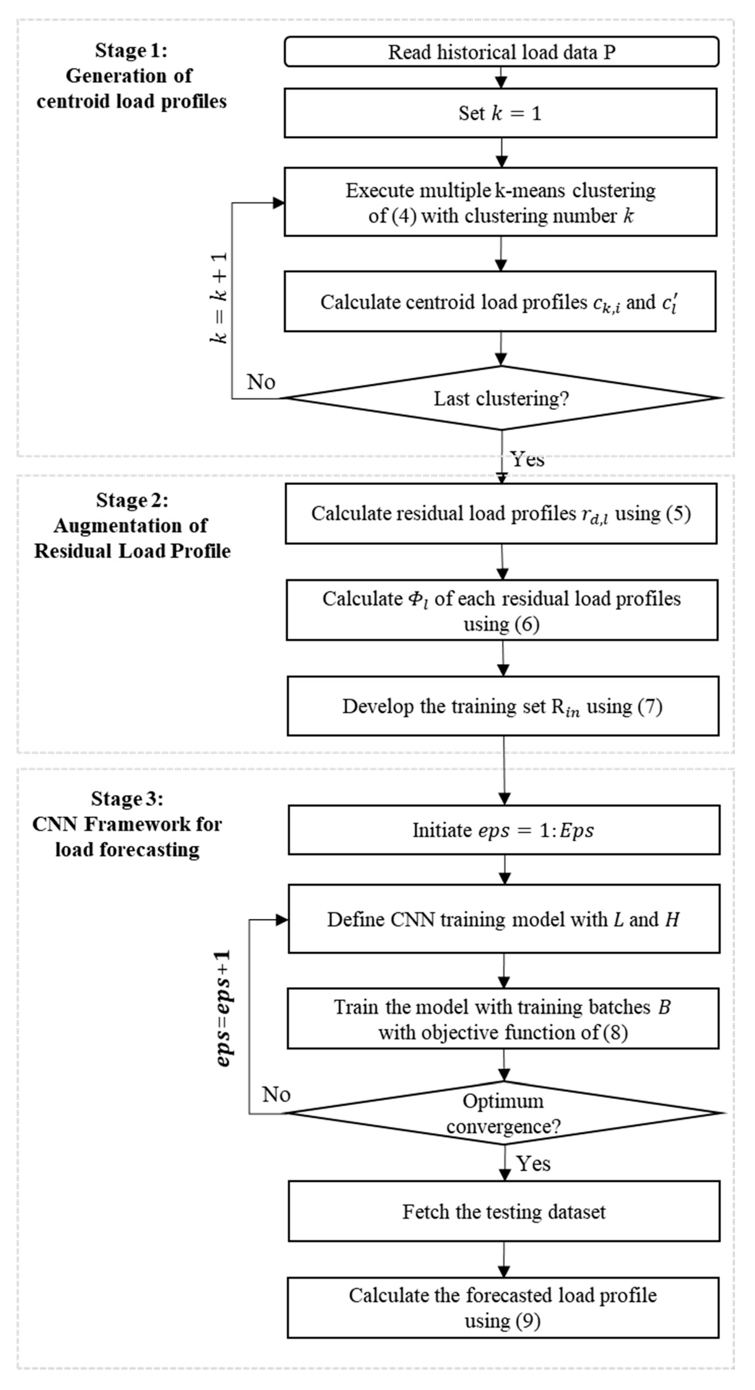
3. Proposed Residential Load Forecasting Method

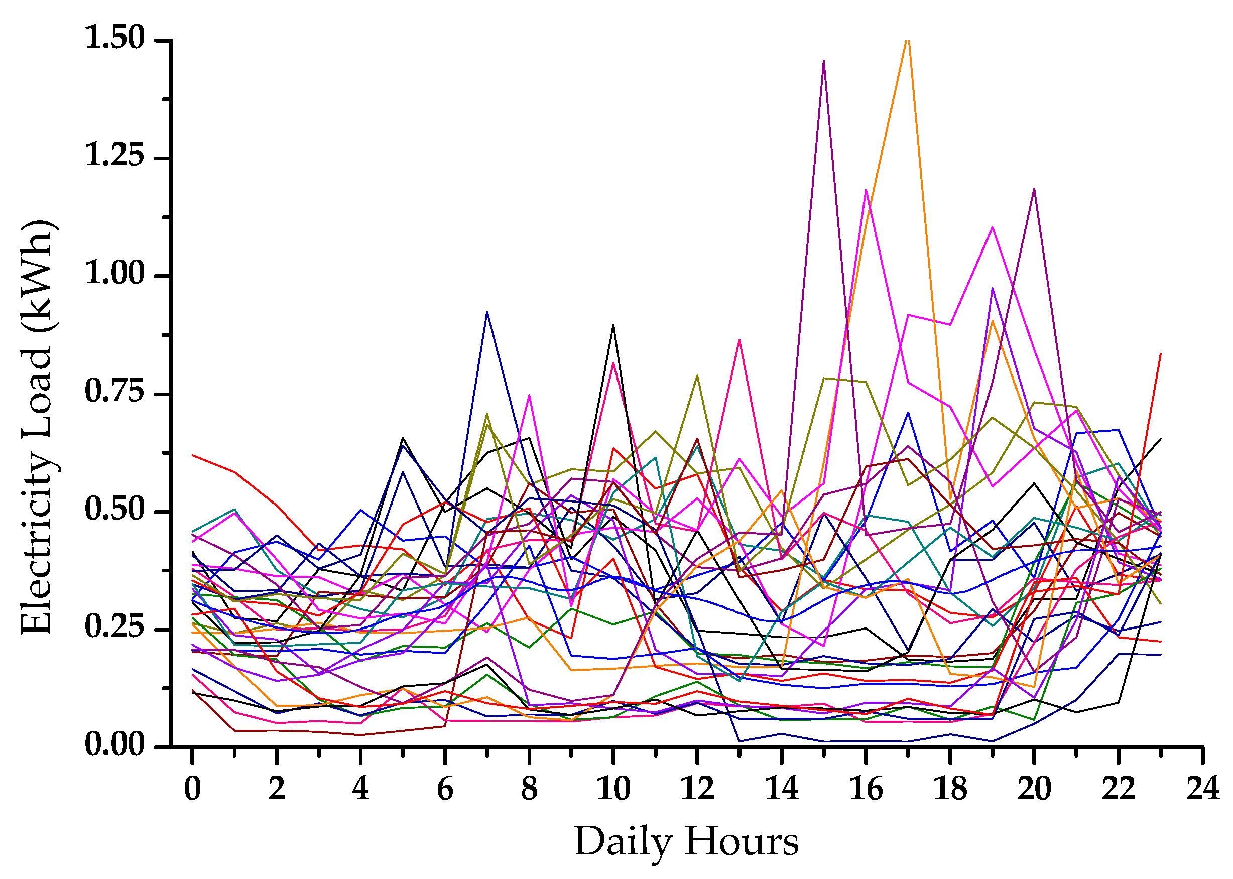
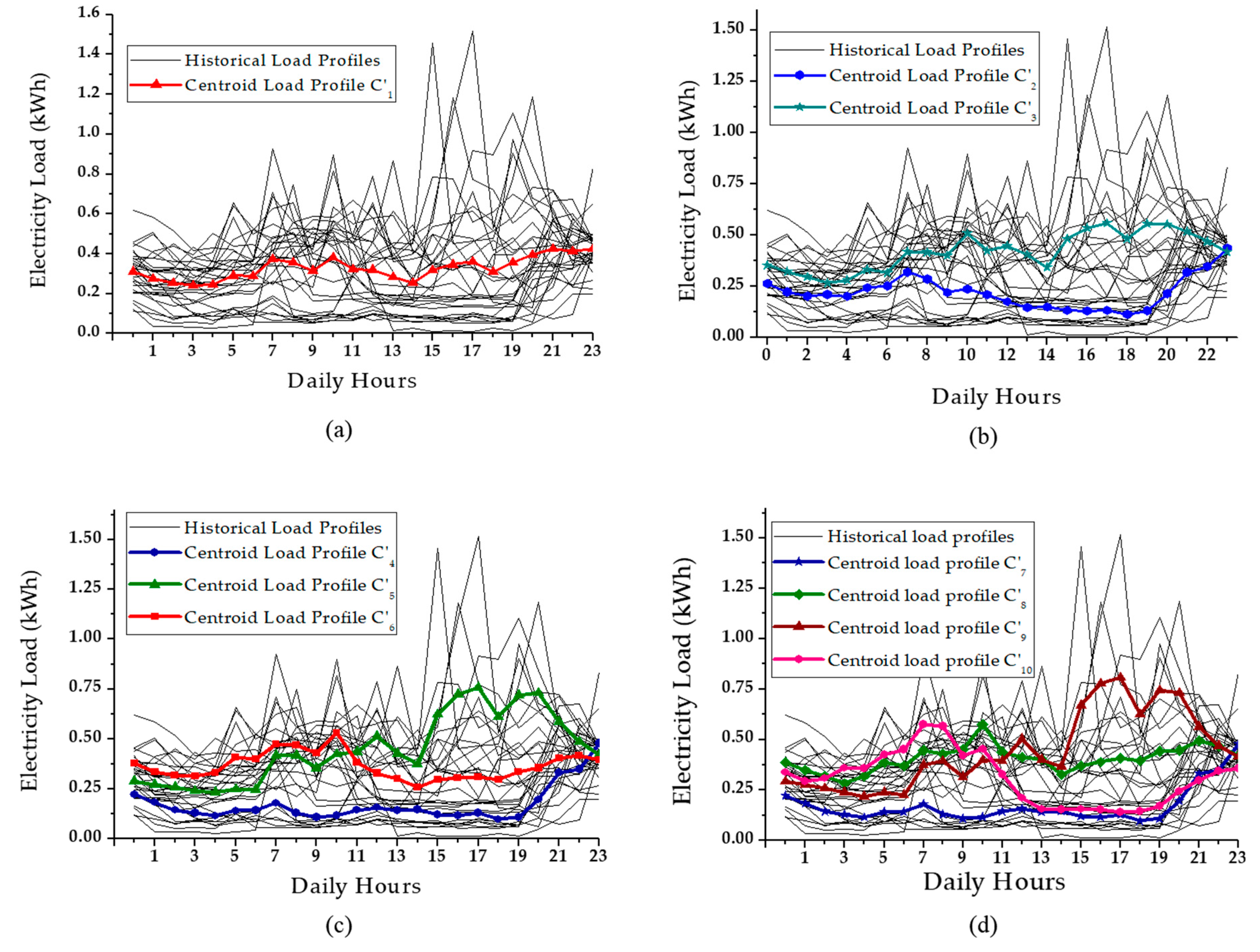
3.1. Generation of Centroid Load Profiles

To generate the different centroid load profiles from historical residential load P, multiple k-means clustering [21,22] is used in the paper. The multiple k-means clustering to generate the centroid load profiles of a residential load can be express as follows:
Minimize     i = 1 k p d S k , i   p d c k , i 2 ,   k = 1 ,   2 , , K ,
where S k , i is the i-th partition of the load profile set P, which is generated with a clustering number of k, and c k , i is the centroid load profile of the corresponding partition of S k ,   i . The clustering starts with a clustering number 1 and ends with the clustering number K . Finally, ( K 2 + K ) / 2 centroid load profiles are generated. The paper used all centroids generated with clustering numbers of one to k, and the l-th generated centroid load profile is defined as c l . The centroid load profiles ( c l ) are ( K 2 + K ) / 2 daily load patterns, which are the mean values of load patterns of similar days. Figure 5 shows the centroid load profiles of a single household for one month using the multiple k-means clustering algorithm.

3.2. Augmentation of Homogeneous Residual Load Profile

Using multiple k-means clustering and its corresponding centroid load profile, the residential load profiles can be generated as follows:
r d ,   l   = p d c l ,
where r d , l   is the vector of residual load profiles of the target household on day d, which is generated with the l -th centroid load profile. This residual load profile is expected to be less volatile and less uncertain than was the original load profile. In addition, from Equation (5), the amount of training data will be increased much more by using residual load profiles as training data. Namely, one time series ( p d ) of a single household load can be transformed into several time series of residual load series ( r d , 1 ,   r d , 2 ,   ,   r d , l ).
For the CNN, the appropriate training data are concatenated with each other, and each training data should have less uncertainty and more homogeneous information. The more homogenous information there is, the more useful it will be for a CNN network to address the granular-level load prediction. Any dissimilar augmented load series could destroy the CNN’s optimal cognition. Therefore, one needs to select the more homogeneous residual load profiles from among the augmented load profiles from Equation (5).
To select the more homogenous residual load profiles, the Frobenius norm [30] Φ l of each residual load profiles are calculated as follows:
Φ l = d = 1 D r d , l   2 ,
where each r d , l   is sequentially observed with time. When residual load profiles ( r d , l   ) have lower Φ l , most residuals generated with c l are closed to its centroid, and these augmented residual load profiles can be expected to be homogeneous. Finally, the paper used only the residual load series with lower Φ l as training set R i n ,
R i n = { r d , l     |   Φ l 1 L l = 1 L Φ l } .
In addition to the training set, the paper used the residual load profiles with the lowest Φ l as the test set for the CNN model. Figure 6 shows the structure of training and testing sets of the proposed method. In Figure 6, the residual load profile is expressed with its elements as r d , l = { r ( 1 , d ) , l , r ( 2 , d ) , l , , r ( t , d ) , l , , r ( 24 , d ) , l } . In the training set, several time series of residual load series ( r d , 1 ,   r d , 2 ,   ,   r d , l ) can be used instead of one original time series ( p d ) of a single household load. With this enragement of training data, forecasting accuracy for individual residential households can be improved.

3.3. CNN Model for Residential Load Forecasting

The training process is yielded by running a program with a given number of iterations. To optimize the CNN model, in each iteration, a root mean square is used for the training process as follows:
argmin   1 L . 1 D . l = 1 L d = 1 D ( r ^ d , l , r d , l ) 2   ,
where r ^ d , l is the predicted vector load profile obtained from the CNN, and L represents the number of selected residual load profiles from Equation (6). A well-trained and converged CNN forecasting network is used for testing the process for predicting the future load. Since the CNN network deals with residual load profiles, the forecasting result can be generated in terms of a residual load profile. In fact, the forecast load profile p ^ D + 1 can be obtained by adding both the centroid load profile and the forecast residual load profile as follows:
p ^ D + 1 = c ^ +   r ^ D + 1 , p ,
where r ^ D + 1 ,   p represents the day-ahead forecasted residual load profile, and c ^ represents the most appropriate centroid load profile which has the lowest Frobenius norm Φ l .
Figure 7 explains the entire load forecasting procedure for the proposed methodology. In the first stage, centroid load profiles are generated using multiple k-means clustering, and different types of residual load profiles are extracted with corresponding centroid load profiles. In the second stage, only homogeneous residual load series are selected using the Frobenius norm for training the CNN. In the final stage, the CNN forecasting framework is used to predict day-ahead residential load profiles. The CNN implementation can be summarized into three parts: (1) initialization of the CNN parameters, (2) training the CNN model with the help of input matrix R i n , and (3) predicting the day-ahead load profile using the optimally trained CNN model. With the proposed forecasting method, it is expected that the CNN can cognize the characteristics of historical load profiles more accurately, so that the forecasting accuracy is improved interestingly.

4. Simulation Results

4.1. Data Description and Hyper-Parameter Tuning

The proposed method was tested using hourly metering data gathered from 1181 residential households in Seoul, Korea, for one year (August 2016 to July 2017). With this dataset, the results of the proposed method are compared with the results of pooling-based augmentation [7] as well as with the results of other deep-learning models [2,7,20]. For the day-ahead load forecasting, historical load data for the last 30 days were used for the training process, and historical load data of the previous day were used for testing. To evaluate the accuracy of forecasting results, the paper employed the mean absolute percentage error (MAPE) and root mean square error (RMSE) as follows:
MAPE = 1 T t = 1 T | p ^ t ,   ( D + 1 ) p t ,   ( D + 1 ) | p t ,   ( D + 1 ) × 100 %   ,
RMSE = 1 T t = 1 T ( ( p ^ t ,   ( D + 1 ) p t ,   ( D + 1 ) ) ) 2   .
The proposed method is developed and tested through Python with the Keras library, whose backend is Tensorflow [31,32]. To avoid over-fitting in the training process, the parameter settings in Table 1 were tested for the proposed method. The tuning process of hyper-parameters was based on [23]. The numbers of hidden layers were selected based on [33,34,35,36,37,38]. The common hyper-parameters, such as activation function, optimizer, loss function, etc., are reported in Table 1. The additional more specific parameters of CNN were settled with the size of filter 3 × 3 , number of input filters 24, maximum pooling size 3 × 3 , and size of strides 1. The convolution layers were followed by a fully connected layer with the rectified linear unit (ReLU) activation functions. The final fully connected layer predicted one-hour electric load at a time, which was matched with [36]. The dataset (30 days) was split into validating set (3 days), testing set (1 day), and training set (26 days).
To tackle the overfitting in CNNs, the proposed method was preliminarily tested with different numbers of hidden layers in CNN architecture. Table 2 shows the forecasting results of ten households with six different hidden layers. The ten single households in Table 2 were randomly selected, and the results were monthly average values in July (peak season in Korea). In most households, the forecasting results with two or three hidden layers were more accurate. With these results, the paper set the number of hidden layers to be 2.

4.2. Effects of Proposed Augmentation Method

Table 3 and Table 4 show the MAPE and RMSE results of day-ahead forecasting with and without the proposed augmentation technique. The ten single households in tested Table 3 and Table 4 were randomly selected, and the results were monthly average values in July (peak season in Korea).
By using the proposed augmentation, the forecasting accuracy was improved by 5 percent, at least, as shown in Table 3. It can be concluded that the proposed forecasting method can significantly improve the forecasting accuracy more than can the other forecasting models without augmentation. When comparing only the cases with the proposed augmentation, the CNN provided more accurate forecasting than the LSTM. It is probably because the augmented data contain plenty of similar random information with small variations. With this information, the CNN received the opportunity for obtaining optimal convergence. On the other hand, as LSTM required more repetitive information for training to improve its performance, this augmented data was comparatively ineffective for LSTM.
Figure 8a,b show the average MAPE and RMSE of ten households, calculated using the results of daily forecasting in July. On most days, the proposed forecasting method significantly improved the forecasting accuracy more than did the other forecasting model without augmentation.
Figure 9 shows the daily average of forecasting results for four higher uncertain households. For most times, the proposed forecasting method significantly improved forecasting accuracy. This is probably because the homogeneous information from the proposed augmentation provides the opportunity for the CNN framework to obtain optimal convergence.

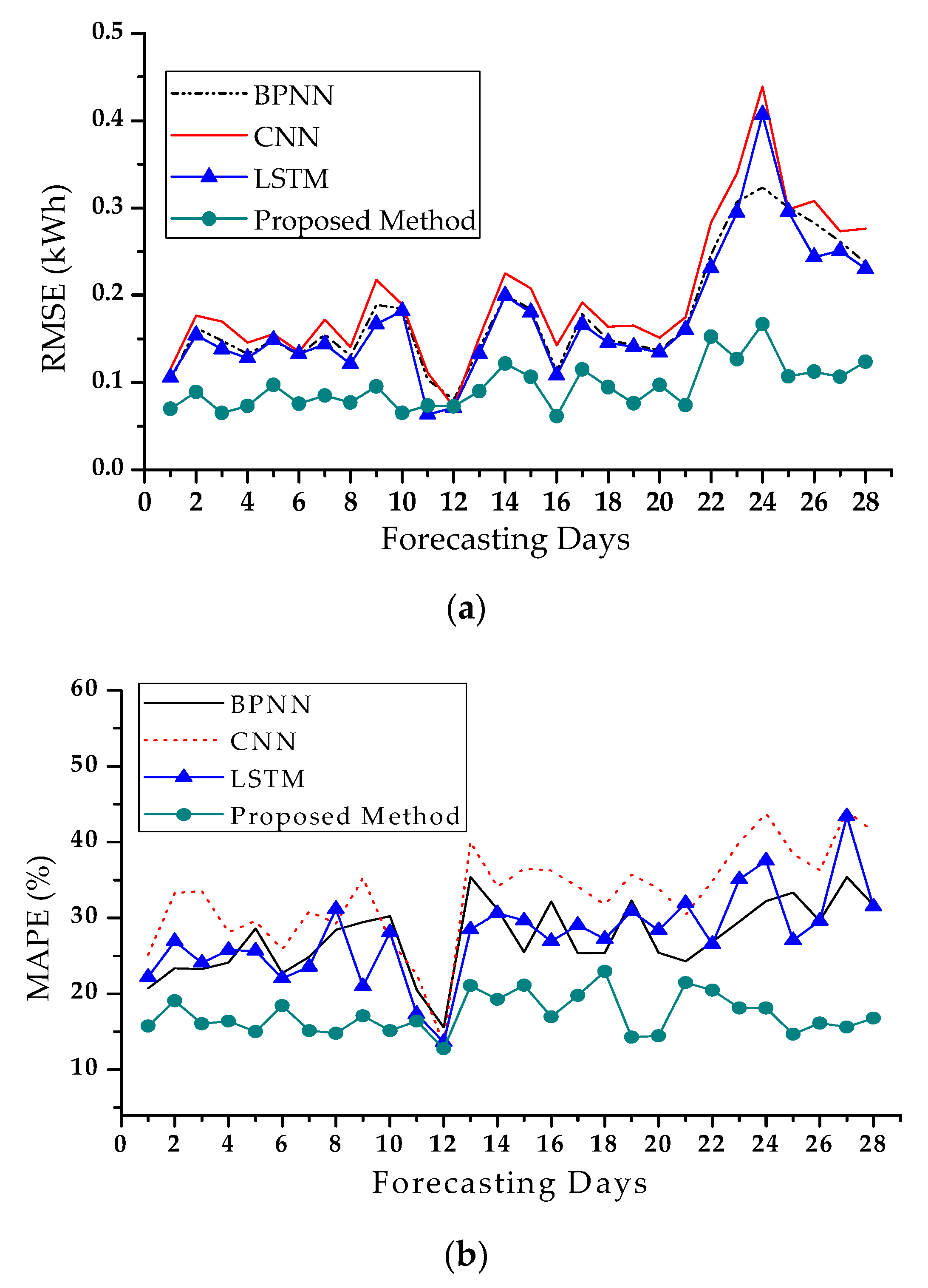
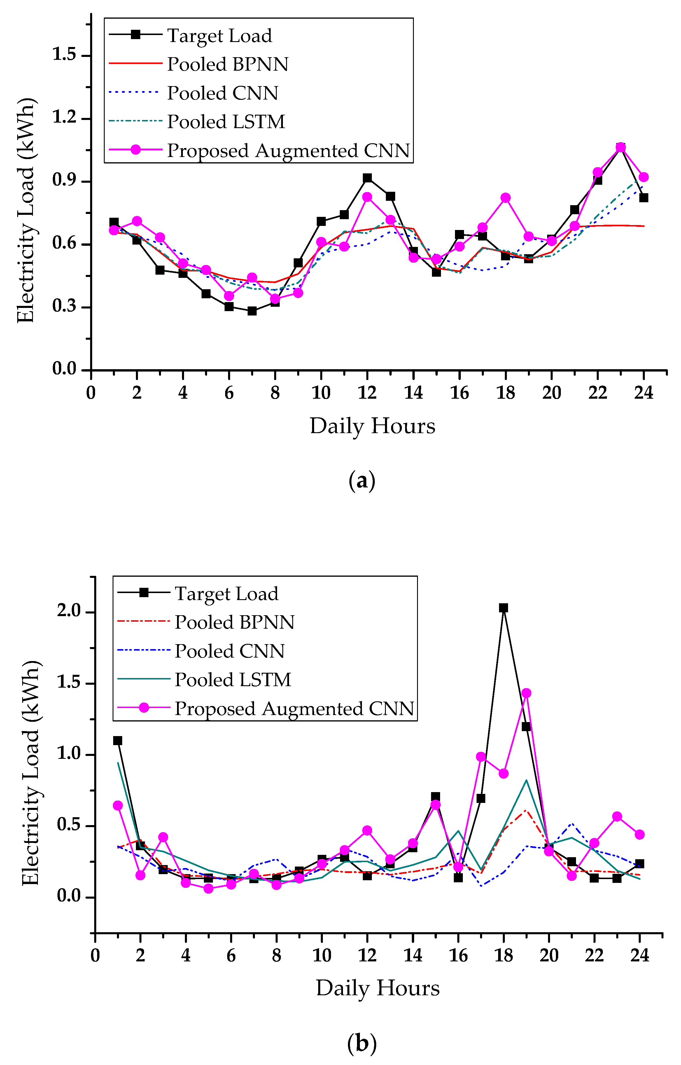
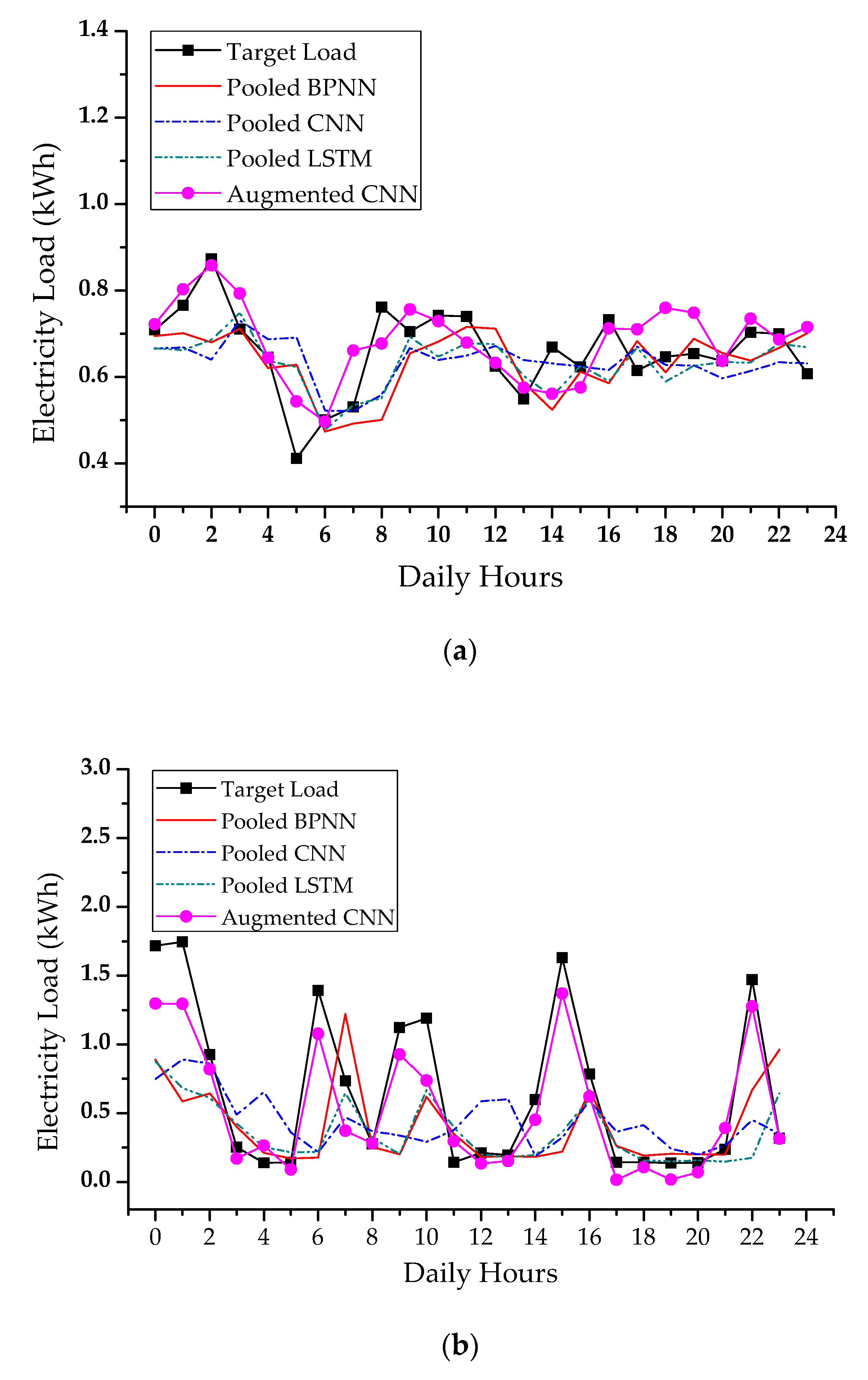
4.3. Forecasting Results in Peak Day

Figure 10a,b show the forecasting results of the peak day for two selected households. One was a less uncertain household which showed the lowest monthly average MAPE in Table 2 (household 4). The other household was a more uncertain household which showed the highest monthly average MAPE in Table 2 (household 10). The peak loads of the two households in July were 1.062 kW (23:00, July 17) and 2.033 kW (18:00, July 14), respectively. During a peak day, it is expected that the residential load profiles will be highly uncertain so that the load forecasting is more challenge. To test the forecasting accuracy, the results of the proposed forecasting method were compared to the results of the forecasting models using pooling augmentation techniques [7].
For pooling augmentation, the simulation used historical load data of six neighbors as an additional training set. In Figure 10a,b, the predicted load curves of the proposed method were much closer to the actual load profile at most hours of the day, for both households. Especially at the peak time of the day, the proposed forecasting model can provide significantly accurate forecasting results. On the other hand, the forecasting models using the other pooling techniques showed a worse performance for load forecasting at the peak time.
An important day for a forecasting test is the day of maximum energy. During this day, the residential load profiles would be highly uncertain at all hours of the day, so that the load forecasting is more challenging. The daily maximum energy consumption of the selected two households in July was 19.381 kWh (July 21) and 15.797 kWh (July 30), respectively. Figure 11a,b demonstrate the target load profile and predicted load profile of the less uncertain household and the highly uncertain household, respectively. For the less uncertain household, the predicted load curves of the proposed method were much closer to the actual load profile at most hours of the day. The proposed model reported 7.999% of MAPE for the less uncertain household, which was lower than the 10.6566% of MAPE from the pooled LSTM. Similarly, for the highly uncertain household, the proposed model reported 40.4058% of MAPE, which was lower than the 53.319% of MAPE from the pooled LSTM. These results strongly validate the proposed methodology for load prediction in the residential sector.

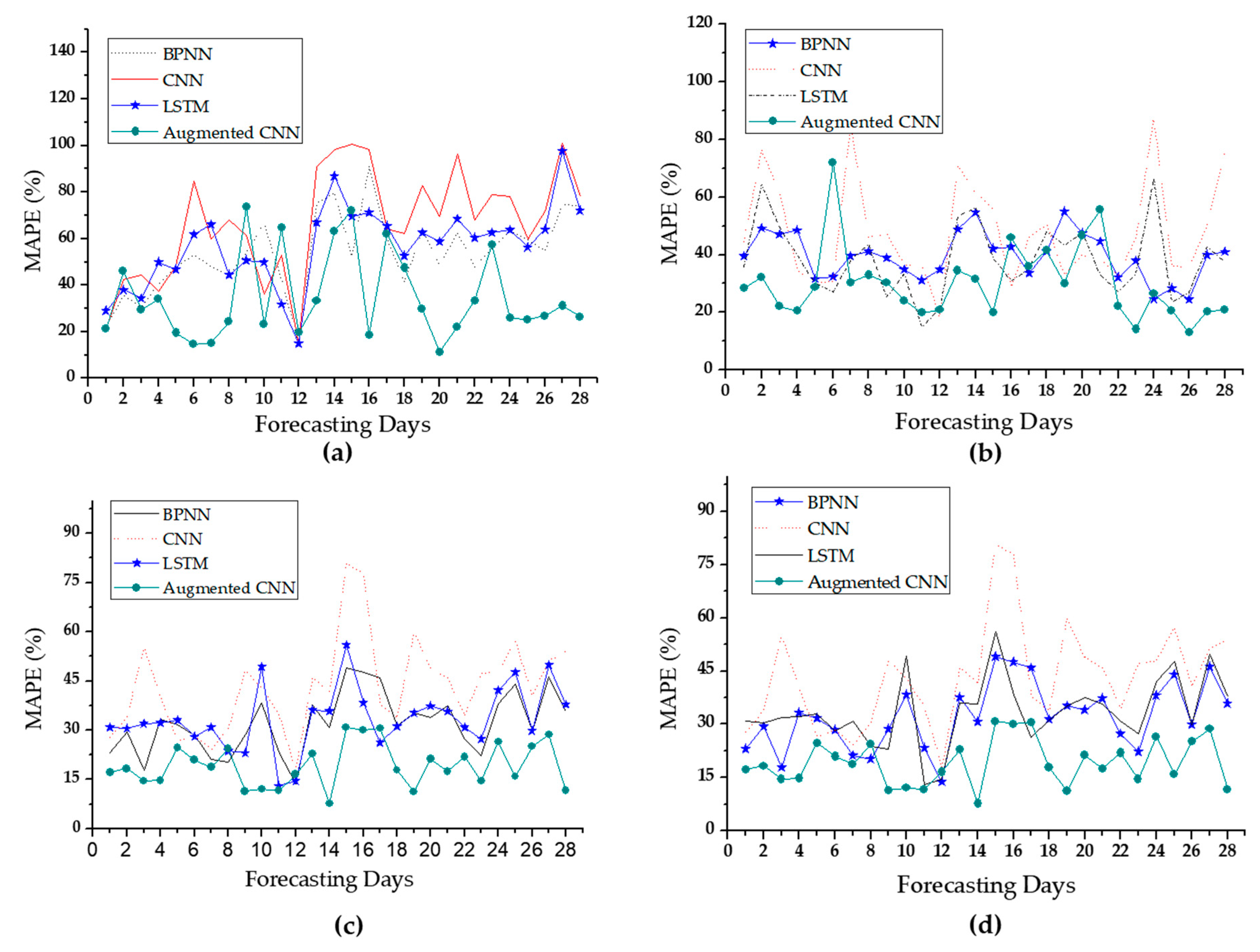
4.4. Monthly Results of Day-Ahead Load Forecasting

To examine the efficacy of the proposed technique for one year, this section tested the performance throughout eleven months by picking one of the best performer households and one of the worst performer households.
Table 5 and Table 6 show the monthly average MAPE and RMSE results of the less uncertain household and the highly uncertain household. The test results are from September 2016 to July 2017. In Table 5 and Table 6, the proposed method improved the forecasting accuracy by more than 6 percent throughout the year.

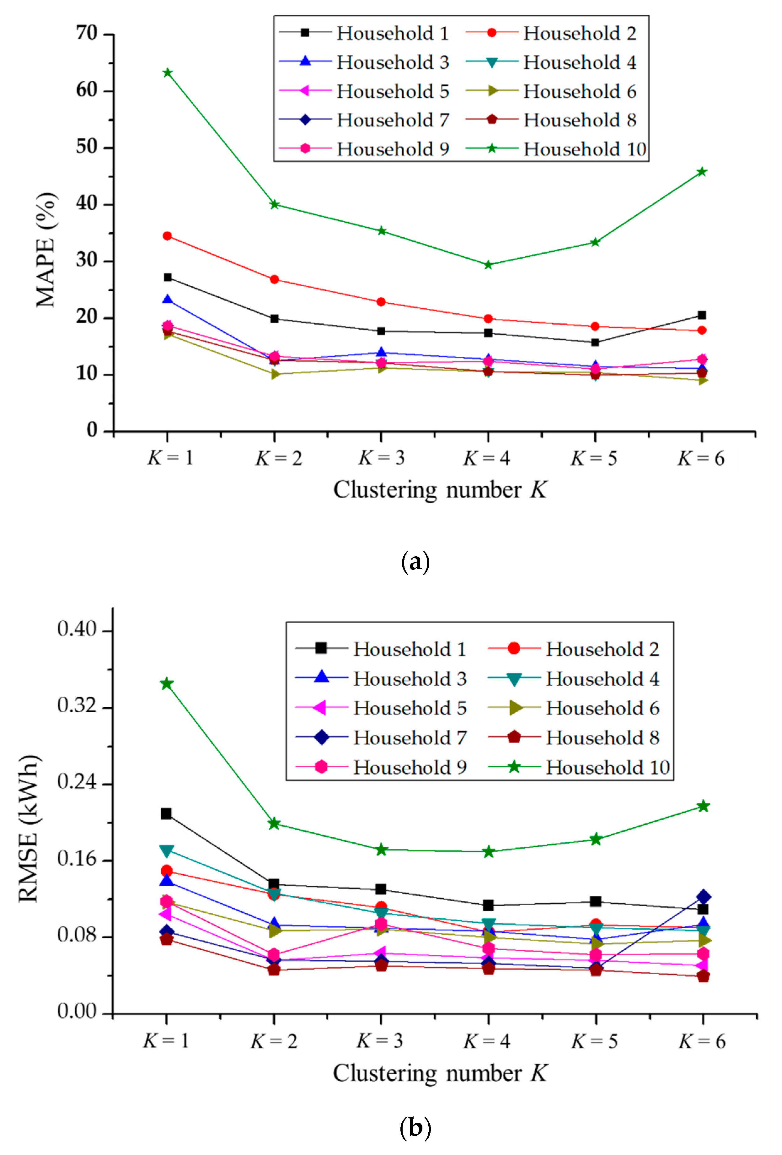
4.5. Impact of Clustering Number K

Figure 12a,b show the average MAPE and RMSE results of ten households with different clustering numbers K . In Figure 12, very accurate forecasting can be expected when the clustering number K is increased for most households. However, for some households, the MAPE is increased when the clustering number K is over 4. The higher clustering number K provides more training data to the CNNs, so that the CNNs have more chance to learn the load characteristics. However, more training data can increase the variations of the training set, which cause overfitting of the hyper-parameters of CNNs, which degrades the optimal learning of CNNs. Therefore, the optimal clustering number must be selected for each household.

5. Conclusions

The paper proposed a forecasting method based on convolution neural networks (CNNs) combined with a data augmentation technique with consideration of an insufficient period of training data. The proposed data augmentation can enlarge the training data for CNNs using only a target household’s own historical data, without the help of other households. The proposed forecasting method transforms a time series of a single household load data into several time series of residual loads. With this enragement of training data, forecasting accuracy for individual residential households can be improved. The test results indicated that the proposed method can deliver a notable improvement by including homogeneous information for an individual residential household’s load forecasting. The proposed method can be used for energy management at the household level and evaluate the baseline of energy consumption at the household level for demand-response programs.

Author Contributions

For research, S.K.A. developed the idea of augmentation strategies for a CNN-based forecasting framework, performed the simulation, and wrote the paper. Y.-M.W. helped organize the article. J.L. provided guidance for research and revised the paper.

Funding

This work was supported by the National Research Foundation of Korea (NRF) grant funded by the Korea government (MSIT) (No. 2017R1C1B5016244). This research was supported by Korea Electric Power Corporation. (Grant number: R18XA04).

Conflicts of Interest

The authors declare no conflict of interest.

References

  1. Shahidehpour, M.; Yamin, H.; Li, Z. Market Operations in Electric Power Systems: Forecasting Scheduling and Risk Management, 1st ed.; Wiley-IEEE Press: New York, NY, USA, 2002; pp. 21–55. [Google Scholar]
  2. Kong, W.; Dong, Z.Y.; Jia, Y.; Hill, D.J.; Xu, Y.; Zhang, Y. Short-Term Residential Load Forecasting based on LSTM Recurrent Neural Network. IEEE Trans. Smart Grid 2017, 10, 841–851. [Google Scholar] [CrossRef]
  3. Charytoniuk, W.; Chen, M.S.; Van Olinda, P. Nonparametric Regression Based Short-Term Load Forecasting. IEEE Trans. Power Syst. 1998, 13, 725–730. [Google Scholar] [CrossRef]
  4. Song, K.-B.; Baek, Y.-S.; Hong, D.H.; Jang, G. Short-Term Load Forecasting for The Holidays Using Fuzzy Linear Regression Method. IEEE Trans. Power Syst. 2005, 20, 96–101. [Google Scholar] [CrossRef]
  5. Christiaanse, W.R. Short-Term Load Forecasting Using General Exponential Smoothing. IEEE Trans. Power Syst. 1971, 2, 900–911. [Google Scholar] [CrossRef]
  6. Mohamed, N.; Ahmad, M.H.; Ismail, Z. Short Term Load Forecasting Using Double Seasonal ARIMA Model. In Proceedings of the Regional Conference on Statistical Sciences 2010 (RCSS’10), Kota Bharu, Malaysia, 13 June 2010. [Google Scholar]
  7. Shi, H.; Xu, M.; Li, R. Deep Learning for Household Load Forecasting-A Novel Pooling Deep RNN. IEEE Trans. Smart Grid 2018, 9, 5271–5280. [Google Scholar] [CrossRef]
  8. Tian, C.; Ma, J.; Zhang, C.; Zhan, P. A Deep Neural Network Model for Short-Term Load Forecast Based on Long Short-Term Memory Network and Convolutional Neural Network. Energies 2018, 11, 3493. [Google Scholar] [CrossRef]
  9. Bouktif, S.; Fiaz, A.; Ouni, A.; Serhani, M.A. Optimal Deep Learning LSTM Model for Electric Load Forecasting using Feature Selection and Genetic Algorithm: Comparison with Machine Learning Approaches. Energies 2018, 11, 1636. [Google Scholar] [CrossRef]
  10. Torres, J.F.; Galicia, A.; Troncoso, A. A Scalable Approach Based on Deep Learning for Big Data Time Series forecasting. In Proceedings of the International Work-Conference on the Interplay Between Natural and Artificial Computation (IWINAC), A Coruña, Spain, 19–23 June 2017. [Google Scholar]
  11. Guo, Z.; Zhou, K.; Zhang, X.; Yang, S. A Deep Learning Model for Short-Term Power Load and Probability Density Forecasting. Energy 2018, 160, 1186–1200. [Google Scholar] [CrossRef]
  12. Lin, Y. Time Series Forecasting by Evolving Deep Belief Network with Negative Correlation Search. In Proceedings of the 2018 Chinese Automation Congress (CAC), Xi’an, China, 30 November–2 December 2018. [Google Scholar]
  13. Vu, D.H.; Muttaqi, K.M.; Agalagaonkar, A.P. Combinatorial Approach using Wavelet Analysis and Artificial Neural Network for Short-term Load Forecasting. In Proceedings of the 2014 Australasian Universities Power Engineering Conference (AUPEC), Perth, Australia, 28 September–1 October 2014. [Google Scholar]
  14. Haq, M.R.; Ni, Z. A New Hybrid Model for Short-Term Electricity Load Forecasting. IEEE Access 2019, 7, 125413–125423. [Google Scholar] [CrossRef]
  15. Gram-Hanseen, G. Standby consumption in households analyzed with a practice theory approach. J. Ind. Ecol. 2010, 14, 150–165. [Google Scholar] [CrossRef]
  16. Du, S.; Li, T.; Gong, X.; Yang, Y.; Horng, S.J. Traffic Flow Forecasting based on Hybrid Deep Learning Framework. In Proceedings of the 12th International Conference on Intelligent Systems and Knowledge Engineering, Nanjing, China, 24–26 November 2017. [Google Scholar]
  17. Wang, Y.; Chen, Q.; Gan, D.; Yang, J.; Kirchen, D.S.; Kang, C. Deep Learning-Based Socio-demographic Information Identification from Smart Meter Data. IEEE Trans. Smart Grid 2018, 10, 2593–2602. [Google Scholar] [CrossRef]
  18. LeCun, Y.; Bengio, Y. Convolution Neural Networks for Images; Speech and Time Series; MIT Press: Cambridge, MA, USA, 1988. [Google Scholar]
  19. Pattanayek, S. Pro Deep Learning with TensorFlow: A Mathematical Approach to Advanced Artificial Intelligence in Python, 1st ed.; Apress: New York, NY, USA, 2017; pp. 153–222. [Google Scholar]
  20. Amarasinghe, K.; Marino, D.L.; Manic, M. Deep Neural Network for Energy Load Forecasting. In Proceedings of the IEEE 26th International Symposium on Industrial Electronics (ISIE), Edinburgh, UK, 19–21 June 2017. [Google Scholar]
  21. Kwac, J.; Flora, J.; Rajagopal, R. Household Energy Consumption Segmentation Using Hourly Data. IEEE Trans. Smart Grid 2015, 5, 420–430. [Google Scholar] [CrossRef]
  22. Wang, X.D.; Chen, R.C.; Yan, F.; Zeng, Z.Q.; Hong, C.Q. Fast Adaptive K-means Subspace Clustering for High-Dimensional Data. IEEE Access 2019, 7, 42639–42651. [Google Scholar] [CrossRef]
  23. Lai, G.; Chang, W.C.; Yang, Y.; Liu, H. Modelling Long-and Short-Term Temporal Patterns with Deep Neural Networks. In Proceedings of the 41st International ACM SIGIR Conference on Research & Development in Information Retrieval, Ann Arbor, MI, USA, 8–12 July 2018. [Google Scholar]
  24. Stephen, B.; Tang, X.; Harvey, P.R.; Galloway, S.; Jennett, K.I. Incorporating Practice Theory in Sub-Profile Models for Short term aggregated Residential Load Forecasting. IEEE Trans. Smart Grid 2017, 8, 1591–1598. [Google Scholar] [CrossRef]
  25. Charalambous, C.C.; Bharath, A.A. A data augmentation methodology for training machine/deep learning gait recognition algorithms. In Proceedings of the British Machine Vision Conference, York, UK, 19–22 September 2016. [Google Scholar]
  26. Lemley, J.; Bazrafkan, S.; Corcoran, P. Smart Augmentation Learning an Optimal Data Augmentation Strategy. IEEE Access 2017, 5, 5858–5869. [Google Scholar] [CrossRef]
  27. Goodfellow, I.; Dengio, Y.; Courville, A. Deep Learning, 1st ed.; The MIT Press: Cambridge, MA, USA, 2016; pp. 224–270. [Google Scholar]
  28. Zhang, Y.; Chen, W.; Xu, R.; Black, J. A Cluster-Based Method for Calculating Baselines for Residential Loads. IEEE Trans. Smart Grid 2015, 7, 1–10. [Google Scholar] [CrossRef]
  29. Farukh, A.; Feng, D.; Habib, S.; Rahman, U.; Rasool, A.; Yan, Z. Short Term Residential Load Forecasting: An Improved Optimal Nonlinear Auto Regressive (NARX) Method with Exponential Weight Decay Function. Electronics 2018, 7, 432. [Google Scholar] [Green Version]
  30. Sharma, T.; Shokeen, D.; Mathur, D. Multiple K Means++ Clustering of Satellite Image Using Hadoop Map Reduce and Spark. Int. J. Adv. Stud. Comput. Sci. Eng. 2016, 5, 23–29. [Google Scholar]
  31. Abadi, M.; Agarwal, A.; Barham, P.; Brevdo, E.; Chen, Z.; Citro, C. Tensor Flow: Large-Scale Machine Learning on Heterogeneous Distributed Systems. arXiv 2016, arXiv:1603.04467. [Google Scholar]
  32. Pedregosa, F.; Varoquax, G.; Gramfort, A. Scikit-learn: Machine Learning in Python. J. Mach. Learn. Res. 2011, 12, 2825–2830. [Google Scholar]
  33. Kong, W.; Dong, Z.Y.; Luo, F.; Meng, K. Effect of Automatic Hyper-Parameter Tuning for Residential Load Forecasting via Deep Learning. In Proceedings of the 2017 Australasian Universities Power Engineering Conference (AUPEC), Melbourne, Australia, 9–22 November 2017. [Google Scholar]
  34. Marino, D.L.; Amarasinghe, K.; Manic, M. Building Energy Load Forecasting Using Deep Neural Networks. In Proceedings of the 42nd Annual Conference of the IEEE Industrial Electronics Society, Florence, Italy, 24–27 October 2016. [Google Scholar]
  35. Ozaki, Y.; Yano, M.; Onishi, O. Effective Hyperparameter Optimization Using Nelder–Mead Method in Deep Learning. IPSJ Trans. Comput. Vis. Appl. 2017, 9, 20. [Google Scholar] [CrossRef]
  36. Torres, J.F.; Troncoso, A.; Gutierrez, D.; Martinez-Alvarez, F. Random Hyper-Parameter Search-Based Deep Neural Network for Power Consumption Forecasting. In Proceedings of the International Work-Conference on Artificial Neural Networks Neural Networks, Gran Canaria, Spain, 12–14 June 2019. [Google Scholar]
  37. Neary, P. Automatic Hyper Parameter Tuning in Deep Convolutional Neural Networks Using Asynchronous Reinforcement Learning. In Proceedings of the 2018 IEEE International Conference on Cognitive Computing (ICCC), San Francisco, CA, USA, 2–7 July 2018. [Google Scholar]
  38. Kim, J.Y.; Cho, S.B. Evolutionary Optimization of Hyper-Parameters in Deep Learning Models. In Proceedings of the 2019 IEEE Congress on Evolutionary Computation (CEC), Wellington, New Zealand, 10–13 June 2019. [Google Scholar]
Figure 1. Comparison of data augmentation strategies: (a) pooling technique and (b) proposed augmentation technique.
Energies 12 03560 g001aEnergies 12 03560 g001b
Figure 2. Daily load profile of a single household for one month.
Energies 12 03560 g002
Figure 3. Average and its residual load series of a single household.
Energies 12 03560 g003
Figure 4. Auto-correlation of residual load series with different time lagging: (a) auto-correlation (AC) coefficients, and (b) partial auto-correlation (PAC) coefficients.
Energies 12 03560 g004
Figure 5. Centroid load profiles generated using multiple k-means clustering algorithm with different clustering number k : (a) k = 1 ; (b) k = 2 ; (c) k = 3 , and (d) k = 4 .
Energies 12 03560 g005
Figure 6. Structure of training and testing data for the proposed method.
Energies 12 03560 g006
Figure 7. The overall procedure of the proposed load forecasting method for an individual household.
Energies 12 03560 g007
Figure 8. Average mean absolute percentage error (MAPE) and root mean square error (RMSE) of ten arbitrary selected households in July: (a) MAPE result, and (b) RMSE result.
Energies 12 03560 g008
Figure 9. Daily average of MAPE of higher uncertain households from Table 3: (a) household 10; (b) household 8; (c) household 9 and (d) household 1.
Energies 12 03560 g009
Figure 10. Day-ahead load forecasting for peak day: (a) lower uncertain household (household 4) and (b) higher uncertain household (household 10).
Energies 12 03560 g010
Figure 11. Day-ahead hourly load forecasting for the day of maximum energy consumption: (a) less uncertain household (household 4) and (b) highly uncertain household (household 10).
Energies 12 03560 g011
Figure 12. Effect of clustering number K on forecasting accuracy: (a) MAPE and (b) RMSE.
Energies 12 03560 g012
Table 1. Hyper parameters for selected deep learning models.
ParametersBPNNCNNLSTM
No. of hidden layers2 or 32 or 3 2 or 3
No. of nodes per layer322420
Activation functionsReLUReLUtanh and sigmoid
No. of Epochs (iteration)150150300
OptimizerRMS-PropRMS-propRMS-prop
Loss FunctionMSEMSEMSE
Testing samples24-h24-h24-h
Table 2. Load Forecasting results (mean absolute percentage error (MAPE)) with a number of different hidden layers.
HouseholdHiddenHiddenHiddenHiddenHiddenHidden
Layer 0Layer 1Layer 2Layer 3Layer 4Layer 5
123.75%24.44%19.26%21.77%23.43%26.77%
211.96%11.25%11.17%9.63%11.51%12.98%
332.10%32.05%30.08%35.87%38.09%39.73%
49.86%9.53%9.65%10.30%11.05%11.47%
513.13%13.59%11.72%12.44%15.47%15.54%
612.88%12.44%11.77%11.43%12.32%13.82%
711.76%11.34%9.77%12.15%11.68%12.82%
814.78%14.97%13.53%14.60%15.12%16.32%
922.19%22.30%22.06%21.41%22.46%21.69%
1037.24%43.59%34.72%46.80%47.12%49.25%
Table 3. Load Forecasting results (MAPE) with and without proposed augmentation.
HouseholdWithout AugmentationWith the Proposed Augmentation
BPNN (%)LSTM (%)CNN (%)LSTM (%)CNN (%)
132.1733.4943.4031.3619.26
220.5421.6224.7716.609.63
339.5238.1548.4837.4130.08
415.5614.6118.4215.479.53
517.3616.5020.8517.1511.72
617.4616.8520.7716.9911.77
714.6114.8517.0113.369.77
820.3820.3124.0818.1713.53
942.4043.1146.0328.8921.41
1053.7157.0266.6451.2834.72
Table 4. Load Forecasting results (root mean square error (RMSE)) with and without proposed augmentation.
HouseholdWithout AugmentationWith the Proposed Augmentation
BPNN (kWh)LSTM (kWh)CNN (kWh)LSTM (kWh)CNN (kWh)
10.36010.34400.40920.31560.1666
20.26140.28640.31690.12530.1116
30.23820.22420.25700.21600.1313
40.09540.09070.11140.13970.0691
50.07900.07680.08820.07440.0506
60.07570.07280.08590.07690.0488
70.06630.06790.07430.06350.0389
80.10830.10280.11600.09600.0683
90.14230.13210.16380.10720.0661
100.33230.30740.34210.29840.1796
Table 5. Monthly-average of MAPE for the lower uncertain household.
Forecasting ModelSept.Oct.Nov.Dec.Jan.Feb.Mar.Apr.MayJun.Jul.
Pooled BPNNMAPE (%)16.4816.7219.3316.5518.2117.3020.9920.2220.8826.9915.02
RMSE (kWh)0.0860.0990.1050.0950.0990.1110.1040.1100.1100.1240.106
Pooled CNNMAPE (%)15.9720.6621.1118.0419.8018.7122.3822.1222.7428.6215.89
RMSE (kWh)0.0850.1110.1160.1040.1100.1210.1120.1190.1200.1320.112
Pooled LSTMMAPE (%)14.4616.3318.2315.3117.3116.7023.3018.7619.9026.8214.03
RMSE (kWh)0.0800.0990.1010.0910.0960.0690.1070.1060.1100.1230.100
Proposed MethodMAPE (%)9.66211.6510.539.509.9110.3411.2510.9512.0712.259.65
RMSE (kWh)0.0620.0610.0600.0600.0610.1050.0670.0750.0720.0680.070
Table 6. Monthly-average of MAPE for the higher uncertain household.
Forecasting ModelSept.Oct.Nov.Dec.Jan.Feb.Mar.Apr.MayJun.Jul.
Pooled BPNNMAPE (%)20.0724.6534.8746.0634.3236.0643.4242.8736.8643.2535.39
RMSE (kWh)0.0860.1190.1370.1560.1600.1680.1850.1910.1410.1520.241
Pooled CNNMAPE (%)18.8028.0834.8355.8039.6137.4448.4953.9040.0950.0741.40
RMSE (kWh)0.0850.1290.1400.1680.1740.1750.2030.2040.1510.1620.246
Pooled LSTMMAPE (%)16.99824.8132.1346.4734.0233.1043.0947.5933.8145.1535.99
RMSE (kWh)0.0800.1160.1350.1560.1640.1610.1760.1980.1400.1530.228
Proposed MethodMAPE (%)13.8312.7922.2630.4723.5122.0926.2130.8923.0529.5329.12
RMSE (kWh)0.0620.0750.0850.1010.0920.1050.1060.1190.0990.0840.131

