Identification of Potential Locations for Run-of-River Hydropower Plants Using a GIS-Based Procedure

Abstract

The increasing demand for renewable and sustainable energy sources has encouraged the development of small run-of-river plants. Preliminary studies are required to assess the technical and economic feasibility of such plants. In this context, the identification of optimal potential run-of-river sites has become a key issue. In this paper, an approach that is based on GIS tools coupled with a hydrological model has been applied to detect potential locations for a run-of-river plant. A great number of locations has been analyzed to identify those that could assure the achievement of different thresholds of potential power. The environmental and economic feasibility for small hydropower projects in these locations has been assessed and a multi-objective analysis has been carried out to highlight the most profitable configurations. The Soil and Water Assessment Tool (SWAT) has been calibrated to simulate runoff in the Taw at Umberleigh catchment (South West England). The results showed that, in the area of study, different locations could be selected as suitable for run-of-river plants.

1. Introduction

Hydropower is currently one of the most cost-effective energy technologies and is the most widely used renewable energy in the world [1,2,3]. Paish et al. [1] analysed the advantages and limitations of hydropower applications, finding that small hydropower plants currently represent the best solution, providing a significant long-lasting and economical source of energy without environmental impacts. Nevertheless, Ranjitkar et al. [2] pointed out that technical and economic issues can be linked to the development of a small hydropower plant and they have to be adequately addressed to ensure reliable installations. Flamos et al. [3] highlighted the importance of including small hydropower plants into an integrated sustainable energy strategy in the context of the occurring climate change.

By the end of 2011, the United Kingdom (UK) generated approximately the 1.5% of its electricity from hydroelectric plants with a total installed capacity of 1676 MW [4]. This percentage represents the 14% of the renewable electricity generated in the country. According to a study that was carried out by Bracken et al. [5], hydropower projects that have been realized in the UK are, in most of the cases, for small scale energy production (less than 100,000 kWh/yea r). In the last years, the number of micro-hydro plants (up to 5 MW installed capacity) increased due to the high efficiency and low costs, mainly in rural areas and small communities [6]. Nevertheless, the potential of hydropower energy is still not completely exploited, especially in small-scale hydropower plants. For these reasons, effective methodologies should be developed and to obtain a correct assessment for small hydropower potential locations in the UK.

Small hydropower is provided, in most of the case, by run-of-river plants. These facilities use the river flow and the drop head (few meters or less of the stream in order to generate electricity). Run-of-river plants are commonly installed with a low dam or a weir to direct water from the river into a penstock linked to a powerhouse, where the potential energy is converted into electricity and the water is released back in the river network. These hydropower plants cannot store water; therefore, their electric production varies with seasonality of river flows.

At a given location, the achievable amount of hydropower is a function of the hydraulic head and the flow rate that depend, respectively, on the local topography and the hydrological processes that occur in the river basin. Therefore, an effective planning of hydropower systems requires a detailed analysis of the area and a proper modelling of river flow. Hydrological models are particularly useful for assessing river flow in ungauged sites. Nevertheless, the modelled river flow needs to be reliable in order to get a correct design of the hydropower systems.

As regards the cost of installation, Paish [1] found that, for small plants up to 500 kW, the costs could vary in a wide range, due to the characteristics of the site; nevertheless, using local expertise and technologies can minimize these costs. Bracken et al. [5] stated that, probably, more than other community-based renewable resources, the costs of small hydropower plants tend to be very dependent on local conditions.

Different steps are involved in the development of a hydropower plant project, including the identification of feasible project locations, and the assessment of river flow, head, and power. The identification of hydropower sites represents a relatively high proportion of overall project costs [7]. For this reason, many efforts have been done in order to define effective procedures to support the project phase of the hydropower site identification. In recent years, GIS tools have been widely used to assess the hydropower potential at the watershed or wider scales. Carroll et al. [8] used GIS tools to identify potential small hydropower sites in the USA. In Thailand, Rojanamon et al. [9] proposed an approach that integrates the GIS application with engineering, economic, environmental, and social criteria, testing the applicability of the method to select hydropower sites in the Nan river basin. Larentis et al. [10] developed a GIS-based computational program for large-scale survey of hydropower potential sites in Brazil. Yi et al. [11] developed and applied a methodology that is based on a Geo-Spatial Information System to detect locations for small hydropower plants in the upper part of Geum River Basin, in Korea. Cyr et al. [12] assessed the small hydroelectric potential for a wide area in Canada while using GIS tools and a regional regression model to evaluate streamflow. Additionally, in Europe, some GIS-based methodologies have been applied to identify hydropower locations [13,14,15]. In Italy, Alterach et al. [13] investigated the potential hydropower resource integrating a numerical technique with GIS tools. Forrest et al. [14] developed a GIS-based algorithm for the identification of potential hydropower sites in Scotland. Gergel’ova et al. [15] used GIS tools to investigate the hydropower potential of the Hornád river basin in Slovakia. More recently, Palla et al. [16] proposed an analytical approach to evaluate the small hydropower potential on a GIS platform. The methodology has been applied and tested on a catchment in Liguria (Italy).

The use of GIS, coupled with a hydrological model for river flow estimation, can effectively improve the identification of hydropower sites. Kusre et al. [17] assessed the hydropower potential of a wide basin in India that couples the use of GIS tools with the Soil and Water Assessment Tool (SWAT) hydrological model, identifying a great number of sites that are suitable for hydropower generation. Goyal et al. [18] used a multi-criteria approach based on the integration of an advanced methodology for preparation of geospatial raster/grid data and the SWAT model in order to detect potential hydropower locations in the Mahanadi river basin (India). Additionally, Pandey et al. [19] used SWAT within a GIS framework in order to assess water availability for hydropower in the Mat River basin, India. The SWAT model has been widely used to simulate the hydrological processes in studies with different purposes, providing reliable estimations of river flow in ungauged basins [20,21,22]. Following the approach that was proposed by Kusre et al. [17] and Goyal et al. 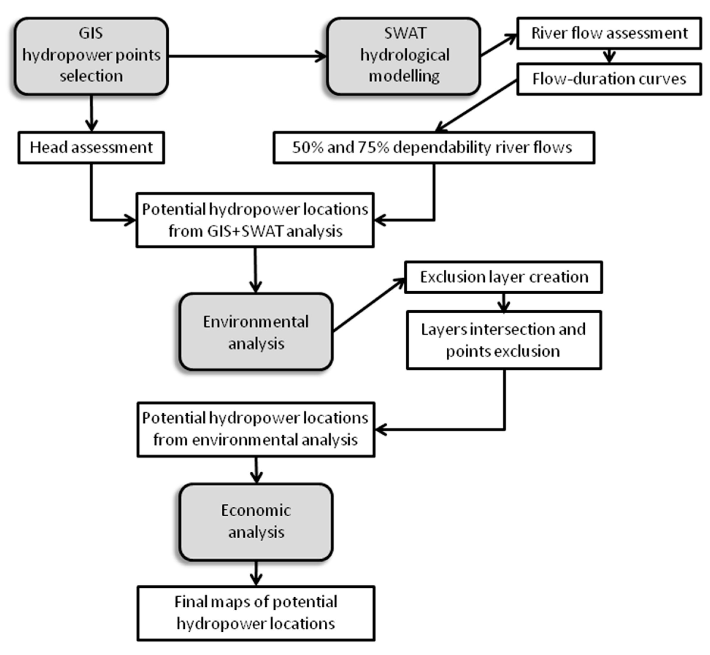[18], in this study, different methodologies that are available in literature have been combined to obtain a procedure for the identification of potential locations for run-of-river plants. Specifically, GIS tools coupled with the application of the SWAT model have been used to identify potential locations for hydropower in the Taw at Umberleigh river basin, in South West England. The SWAT model has been calibrated and applied to evaluate river flow in several sub-basins of the above-mentioned watershed. Thus, the variability of flow along the river network has been assessed. An environmental and an economic analysis have been carried out once the potential locations have been detected. An exclusion layer has been created in GIS to filter out points located in areas that have environmental constraints. For the selected locations, the economic payback has been calculated to provide an assessment of the economic feasibility of run-of-river projects in these sites. The results have been provided in some maps showing the potential locations of hydropower for different ranges of potential power and the related payback period in years. The procedure here proposed turned out to be a valuable support for decision-makers in the preliminary identification of the most suitable sites for run-of-river plants installation in the area of study due to the integration of hydrological, environmental and economic aspects.

2. Case of Study and Dataset

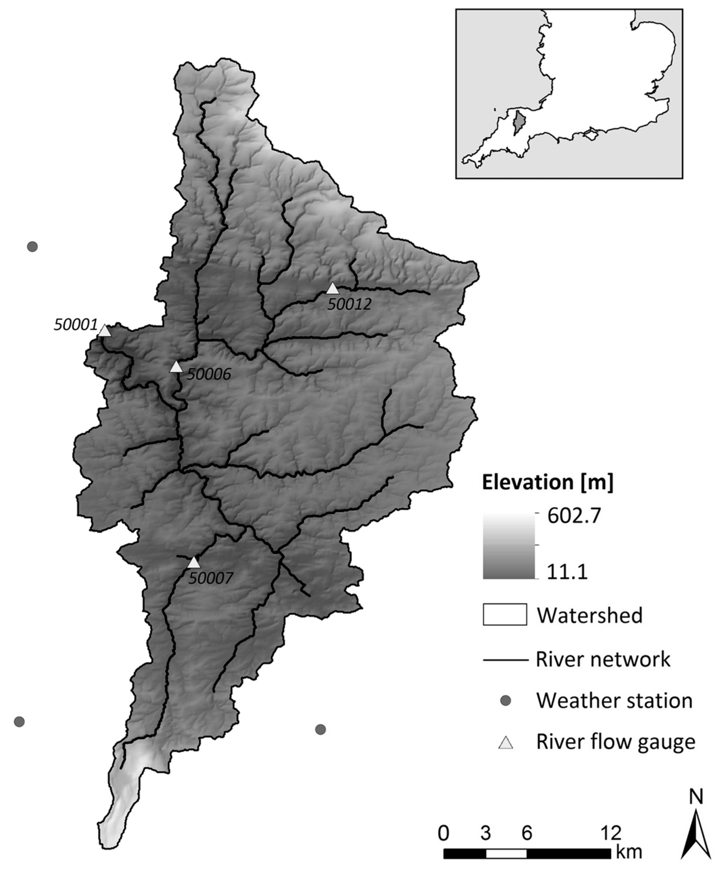
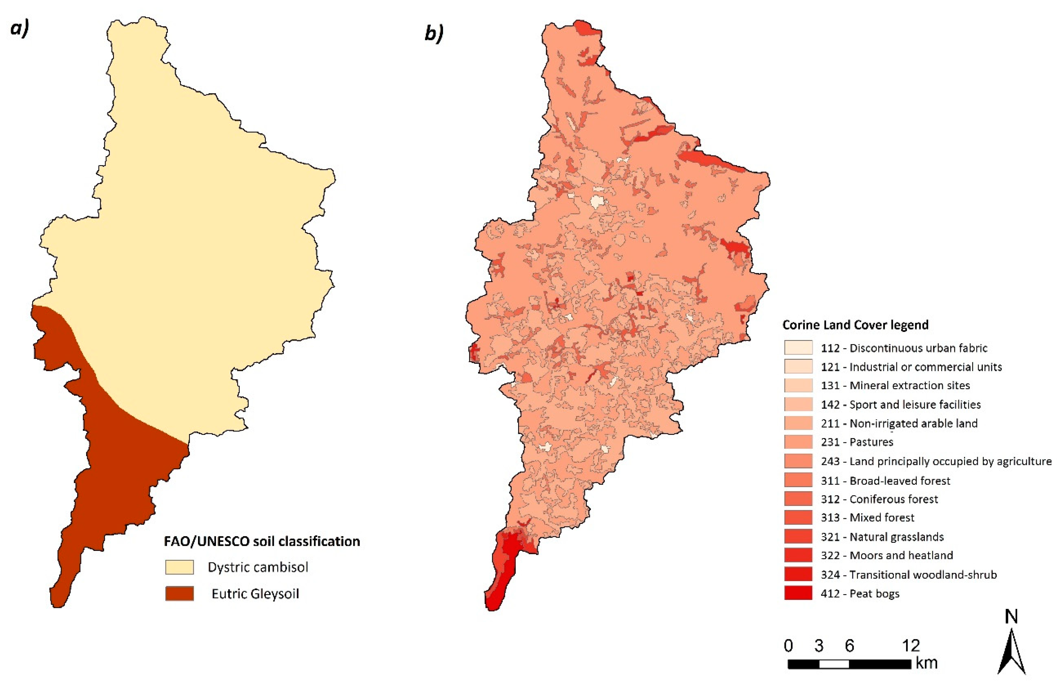
The study area is the Taw at Umberleigh river basin, which is located in South West England (Figure 1). The catchment surface is about 830 km². The most frequent land cover is grassland (60%), whereas croplands take up the 22% of the area. The remaining catchment surface is covered by woodlands (16%) and urban areas (2%). In the basin, there are two predominant soil types: the Dystric Cambisols and the Eutric Gleysol covering, respectively, 82% and 18% of the area.

According to the Köppen classification, the climate of South West England is classified as oceanic, being typically characterized by warmer summers, cool winters, and precipitation evenly distributed during the whole year. Average annual rainfall ranges between 1200 and 1400 mm/year. Average annual temperature is about 10 °C. July and August are the warmest months in the region, with an average annual temperature of about 15–16 °C.

The application of the procedure described in the following sections required, for the area of study, weather time series and spatial data, including topography, land cover, and soil information. Daily series of precipitation, temperature, solar radiation, relative humidity, and wind speed data, recorded by the weather stations shown in Figure 1, have been collected from the global dataset of National Centers for Environmental Prediction (NCEP) Climate Forecast System Reanalysis (CFSR). The authors have referred to the Global Weather Data for SWAT website (http://globalweather.tamu.edu/) in order to get these data directly in the format required by the SWAT model. Daily river flow data for SWAT calibration and validation have been provided by the National River Flow Archive of the United Kingdom (NRFA). Figure 1 shows the locations of the river basin gauges used in this study. The ID number of these gauges refers to the NRFA classification. The model has been calibrated while using daily data recorded at the 50001 gauge (located at Umberleigh, the catchment outlet), while data that were recorded in the remaining gauges (50006, 50007, 50012) have been used to verify the reliability of the obtained results.

The Digital Elevation Model (DEM) for the area of study has been extracted from the Ordnance Survey’s OS Terrain 50 product (50 × 50 m), downloaded from the EDINA Digimap OS service. The soil map of the river basin has been extracted from the FAO/UNESCO Soil Map of the World, whereas the Corine Land Cover 2012 map has been used to obtain information regarding land use in the area of study. Figure 2a,b show, respectively, the soil and the land cover maps of the area of study.

3. Methods

3.1. Procedure Overview

The procedure developed in the present work is illustrated by the flowchart in Figure 3 and it involves the following steps:

• Firstly, by means of GIS tools, potential run-of-river locations have been selected in the DEM, according to the criteria that will be described in detail in Section 3.3;
• Once the sites to be analyzed have been selected, the SWAT model has been applied to each of these points to obtain a reliable estimation of daily river flows for flow-duration curve assessment;
• Based on head and river flow values, a preliminary site assessment has been carried out, considering four different power thresholds;
• An exclusion layer has been created in GIS to filter out points located in areas that have environmental constraints; and,
• For the locations obtained from the environmental analysis, the economic feasibility has been assessed following the procedure that is described in Section 3.7.

3.2. Estimation of Hydropower Potential

The potential source of hydropower is affected by water river flow Q, the total net head H_n between the inlet and outlet section of the turbine and by the turbine efficiency η. Q is evaluated by means of a rainfall-runoff model and the drop head is estimated from the DEM as height difference along the riverbed, while neglecting the energy losses along the penstock. The turbine efficiency depends on the characteristic curve of the turbine for a given supply condition (Q and H_n) and, also, depends on the kind of turbine installed in the hydropower plant [1,23,24,25,26]. There are many types of turbines and the selection of the most appropriate is an important part of the design process. Pelton and Turgo turbines are frequently used for high heads (>50 m) and small flow rates, Crossflow and Francis are more common when the head is lower than 50 m in a wide range of flow rate, and Kaplan are used when the head is lower than 10 m and the flow rate is high [1,25].

The amount of power that is generated by the power plant for given flow conditions is estimated by using the following equation:

$$P=\eta ·\rho ·g·Q·H_n$$

(1)

where P is the generated electric power in watt, ρ is the density of water (1000 kg/m³), g is the gravitational acceleration (9.81 m/s²), Q is the river flow rate in m³/s, H_n is the net head in meters, and η is the overall efficiency of the hydropower plant. In this phase of the study, the analysis has been focused on the potential power of the hydroplant, therefore the generated electric power has been estimated by setting the total hydropower efficiency of the plant $\eta$ equal to 1.

3.3. DEM Analysis and Hydropower Points Selection

The DEM of the river basin has been analyzed in order to detect suitable hydropower sites. Specifically, the 50 × 50 m DEM has been used to delineate the stream network, to calculate the length of the river channels, to evaluate the river bed slope, to identify the sub-basins areas, and, finally, to assess the elevation of a great number of points along the river network (intersecting the DEM raster with the points layer). River channels have been ordered following the Strahler method [27].

The river network layer has been compared with that viewable in the OpenStreetMap (https://www.openstreetmap.org) and the British river network freely downloadable from the Ordnance Survey website (https://www.ordnancesurvey.co.uk/) in order to validate the river network delineated, starting from the DEM, by means of GIS tools. The comparison showed that the river network layer used in this work corresponds with the effective river network.

For the selection of the potential sites for a run-of-river project, the following criteria have been adopted:

• To assure a sufficient river flow, only channels that have flow accumulation of 10,000 cells (50 × 50 m) or more have been considered; and,
• For each site, it has been assumed that the maximum distance of the site from the hydropower station was 100 m. The reasons for this choice are related to hydrological, ecological, and economic aspects. First of all, if the water that is diverted from the river channel is released back as close as possible to the diversion point, the implications on river flow regimes will be minimized and, consequently, also those on river ecosystems. Moreover, a shorter length of the pipeline will reduce the costs that are related to the plant installation.

The river network has been subdivided into segments 100 m long, starting from the highest elevation to the lowest. Each couple of two consecutive points identifies a segment of the river for a potential hydropower plant. The starting point of the segment is the point where the water is diverted to the power plant, and the ending point of the segment is the section where the water is released back in the river. The ending point of the examined segment of the river becomes the starting point of the next segment to be analyzed.

Once the sites have been selected according to the above-mentioned criteria, the hydrological model has been calibrated using data that were recorded at the outlet of the catchment (the 50001 gauge, located at Umberleigh), and then applied to calculate the daily river flow in the selected locations. Successively, the potential power in each of these sites has been assessed while using Equation (1).

3.4. Rainfall-Runoff Modelling

SWAT is a continuous and long term hydrologic model that was developed by the United States Department of Agriculture–Agricultural Research Service (USDA–ARS) with the aim of predicting the impact of agricultural or land management on water resources, sediment, nutrient, and pesticides yields in ungauged basins [28]. It is a physically-based hydrological model with distributed parameters that are able to simulate the hydrologic cycle processes at daily, monthly or annual time step. As input, the model requires the historical measurement of weather data (precipitation, temperature, solar radiation, relative humidity, and wind speed) and the map of topography, land cover, and soil for the area of study. SWAT divides the basin into many sub-basins, which are in turn partitioned into Hydrological Response Unit (HRUs), spatial units with homogeneous soil, land use, and slope characteristics. The model simulates the response of each HRU in terms of water quantity and quality then results are aggregated at the sub-basin scale and routed to the watershed outlet through the channel network. The hydrological model is based on the following water balance equation for soil water content:

$$S{W}_t=S{W}_{t-1}+P_t-Q_t-E{T}_t-S{P}_t-Q{R}_t$$

(2)

where $S{W}_t$ is the soil water content for the current time step, $S{W}_{t-1}$ is the soil water content for the previous time step, $P_t$ is the precipitation, $Q_t$ is the surface runoff, $E{T}_t$ is the evapotranspiration, $S{P}_t$ is the percolation or the seepage, and $Q{R}_t$ is the return flow.

In this study, the QGIS interface of the model, called QSWAT [29], has been used. This interface is provided with tools for stream network and watershed delineation, sub-basins definition, and the identification of the HRUs. For the area of study, SWAT has been calibrated while using the software package SWAT-CUP [30]. Among the available procedures in the tool, the Sequential Uncertainty Fitting algorithm (SUFI-2) has been applied for sensitivity analysis and calibration. A sensitivity analysis has been carried out to identify the parameters that are most influential in governing streamflow response. The model has been calibrated using the river flow series measured at the Umberleigh outlet. The available observed data has been divided into two datasets, the first for calibration and the second for validation. The performance of the model has been evaluated by means of the Nash and Sutcliffe coefficient of efficiency $E_{NS}$ [31], which indicates the degree of fitness of observed and simulated data:

$$E_{NS}=1-\frac{{\sum }_{t=1}^T{\left(Q_0^t-Q_m^t\right)}^2}{{\sum }_{t=1}^T{\left(Q_0^t-\overline{Q_0}\right)}^2}$$

(3)

where $Q_0^t$ is observed value of streamflow, $Q_m^t$ is the simulated value of streamflow, and $\overline{Q_0}$ is the average of the observed values of streamflow. The value of $E_{NS}$ ranges from 1 (best simulation) to negative infinity. To assess the model performance, the coefficient of determination R² has also been calculated.

Once the SWAT model has been calibrated and validated, it has been applied to estimate the river flow in several points along the river network. Model calibration involves the identification of the best set of SWAT parameters in terms of goodness of fit. Basically, the SWAT parameters are optimized until the difference between simulated and measured river flow is satisfactory.

3.5. Flow-Duration Curves

For each of these points, the simulated series have been used to construct the flow-duration curve. Flow-duration curves are of interest for many hydrological applications [32] and they are frequently used in the design of run-of-river plants [33]. A flow-duration curve indicates the percentage of time that the river flow is expected to equal or exceed some given values. The construction of the flow duration curve is based on the following steps:

• Ranking of the river flow series from smallest to largest;
• Calculation of the cumulative frequency of river flow; and,
• Plotting of the ordered series against the corresponding cumulative frequency.

The flow-duration curve allows for one to estimate the river flow corresponding to different degrees of dependability. In this study, the hydropower of the potential sites has been evaluated while considering the 50% and the 75% dependability river flow values [17,19].

3.6. Environmental Analysis

The EU Water Framework Directive specifies a number of environmental and ecological factors that have to be considered in the planning and development of hydropower projects to assure the protection of the aquatic ecosystems and the water quality of the rivers. In the UK, the development of hydropower projects will also require environmental permits from the Environment Agency. The Environment Agency is less likely to accept projects proposals in locations of high environmental sensitivities, such as protected sites or sites where there are protected species. Therefore, only schemes that are well designed to prevent any negative impact on river wildlife and ecosystems could obtain the required permits. The implementation of measures aimed at the reduction of environmental impacts (e.g., installation of fish passages to maintain migration patterns) could remarkably increase the cost of plant realization.

Sites that are located in protected areas are likely to result unsuitable for run-of-river plants or could not be developed to their theoretical potential due to environmental concerns and increased costs. For these reasons, these sites have been excluded from the analysis. To this aim, an exclusion layer has been created in GIS while considering the areas that have environmental constraints. Namely, this layer (Figure 4) has been obtained by the intersection of the following maps (all published by Natural England Open Data):

• The Priority River Habitat map, including rivers and streams that exhibit a high degree of naturalness. This map should be used to identify river channels where particular measures are needed to protect the naturalness of river systems;
• The National Parks map of England; and,
• The Site of Special Scientific Interest map, which includes areas that are characterized by the presence of wildlife or natural features to be protected.

3.7. Economic Analysis

According to the cost formula that was proposed by Ogayar and Vidal [34], the cost of electro-mechanical equipment C of a hydropower plant can be generally expressed as a power function of the power P and the head H:

$$C=a·P^b·H^c$$

(4)

where a, b, and c are coefficients, depending on the geographical location.

Starting from previous studies results, Gallagher et al. [35] proposed some values for the above-mentioned coefficients valid for calculating turbine/generator costs of different turbines (Pelton, Francis and Kaplan) in the UK. In this study, these coefficients have been used to assess the plant costs. The obtained costs have been increased to 10% in order to take into account for maintenance costs [26].

Once costs have been estimated, the economic payback EP for turbine and generator (years) has been calculated while using the following expression [35]:

$$EP=\frac{C}{tp·i}$$

(5)

where tp is the total power output over one year (kWh) and i is the income (€/kWh) from feed-in tariffs (FITs).

4. Results

4.1. Stream Characterization

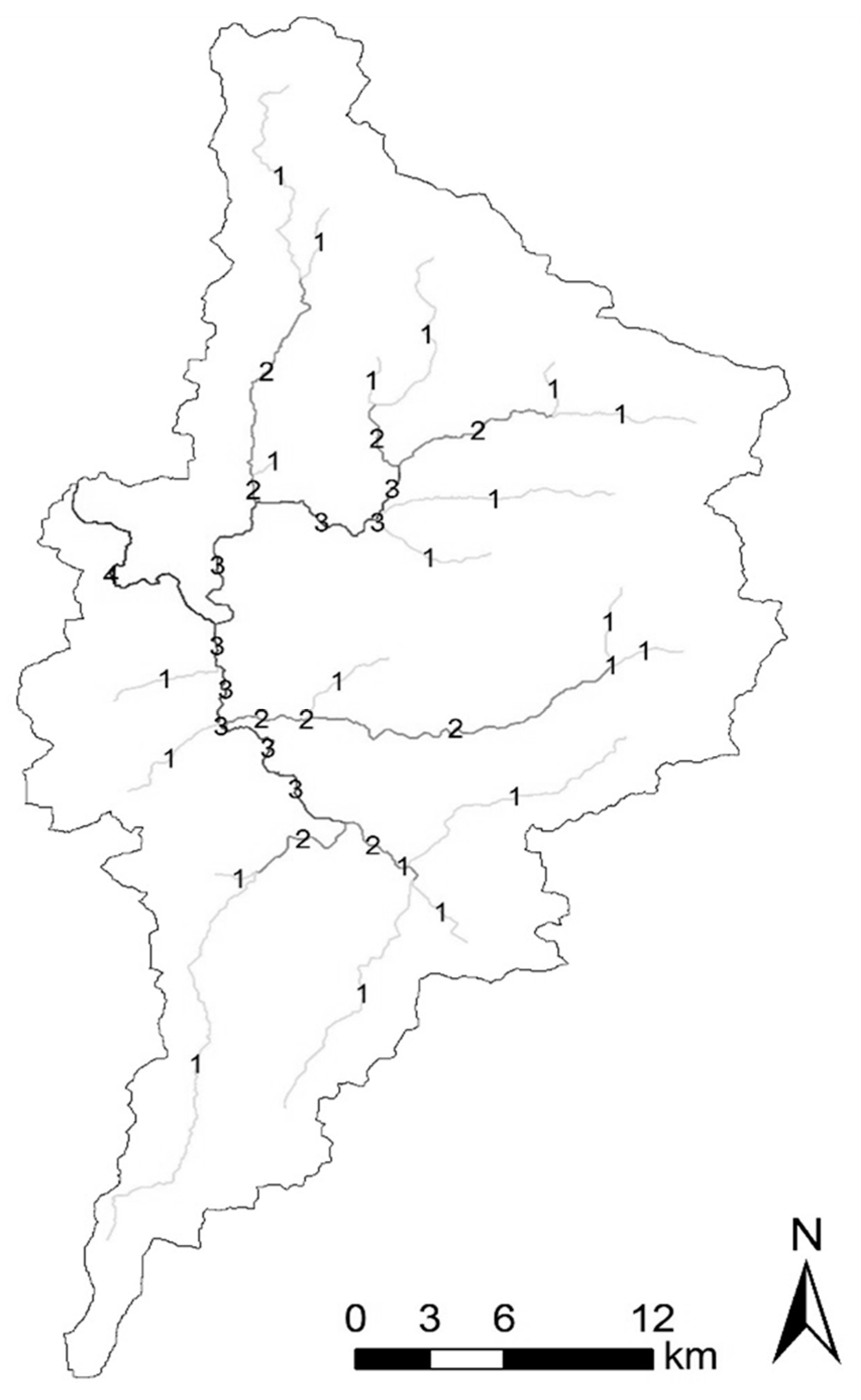
According to the Strahler method, the maximum river channels order is 4. In the river network, 60 stream channels of a different order have been identified and analyzed. Figure 5 shows the order of each channel. The 57% of the stream channels have order equal to 1, while the 23%, the 14% and the 6% have order equal to 2, 3, and 4, respectively. The average length of the channels is approximately 4 km. The channel of order 4 is 20 km long. The highest point of the river is at 356 m, while the lowest is at 14 m. The river bed slope ranges between 0% and 5%.

The application of the procedure previously described allowed for detecting 2189 locations along the river network. The 56% of these points are located along channels of order 1, while the 24% and the 15% of these points are along channels of order 2 and 3, respectively. Only the 5% of points are located in the stream channel of order 4.

4.2. Evaluation of River Flow

River flow data are required to assess the potential hydropower of a site. The lack of data availability represents a limitation for the design of hydropower plants that can be effectively overcome by applying a hydrological model.

The study area has only four river gauging sites. For this reason, a well-calibrated model has been required for assessing the river flow in different ungauged sites along the river network. The SWAT model has been calibrated while using river flow data that were measured at the 50001 outlet during the period 2000–2006 and validated using data that were recorded from 2007 to 2013. Calibration and validation have been performed at the daily scale. The CFRS weather data (as mentioned in Section 2) were used as input. The reliability of the CFRS dataset in SWAT calibration and applications has been widely discussed in previous studies [36,37,38].

A sensitivity analysis has been carried out to identify the parameters that mainly affect model output. Among the model parameters, ten were identified to be the most sensitive (

Table 1. Ranges for model calibration and final value of Soil and Water Assessment Tool (SWAT) parameters (ordered from the most sensitive to the least).

Parameter	Description	Range	Measurement Unit	Calibrated Value
ESCO	Soil evaporation compensation factor	0.01–1	−	0.232
REVAPMN	Threshold depth of water in the shallow aquifer for revap to occur	0–500	mm	495.075
GW_DELAY	Groundwater delay time	0–450	day	5.025
SURLAG	Surface runoff lag coefficient	0.05–24	−	4.510
ALPHA_BF	Base flow alfa factor	0–1	day−1	0.648
GWQMN	Threshold depth of water in the shallow aquifer required for return flow to occur	0–5000	mm	0.283
GW_REVAP	Groundwater “revap” coefficient	0.02–0.2	−	0.178
RCHRG_DP	Deep aquifer percolation fraction	0–1	−	0.195
CH_K2	Effective hydraulic conductivity in main channel alluvium	0.01–500	mm/h	1.739
CH_N2	Manning roughness for main channel	0.01–0.3	−	0.122

). According to sensitivity analysis results, ESCO (soil evaporation compensation factor) is the most sensitive parameter, while variations of CH_K2 (effective hydraulic conductivity in main channel alluvium) and CH_N2 (Manning roughness for the main channel) are affecting model output less than other parameters. REVAP_MIN (threshold depth of water in the shallow aquifer for revap to occur) and GW_DELAY (groundwater delay time) are also sensitive parameters.

Figure 6a,b show the comparison between the observed and simulated river flow series for the calibration at the daily and monthly scale, respectively. The simulated river flow shows good agreement with measured values in both cases. Specifically, the $E_{NS}$ coefficients for streamflow was 0.85 for the calibration period and 0.80 for the validation period.

Table 2. Statistical indexes, E_NS, and R² of the observed and simulated series for model calibration and validation.

Parameter	Calibration		Validation
	Observed	Simulated	Observed	Simulated
Average (m3/s)	17.9	15.5	18.5	14.9
Standard deviation (m3/s)	15.7	13.7	24.4	11.9
Maximum (m3/s)	134.6	119.2	258.0	199.7
ENS	0.85		0.80
R2	0.88		0.85

shows the comparison between the statistical indexes, the E_NS and the coefficient of determination R² of the observed and simulated river flow, respectively. Table 1 shows the set of parameters that provides the best model performance.

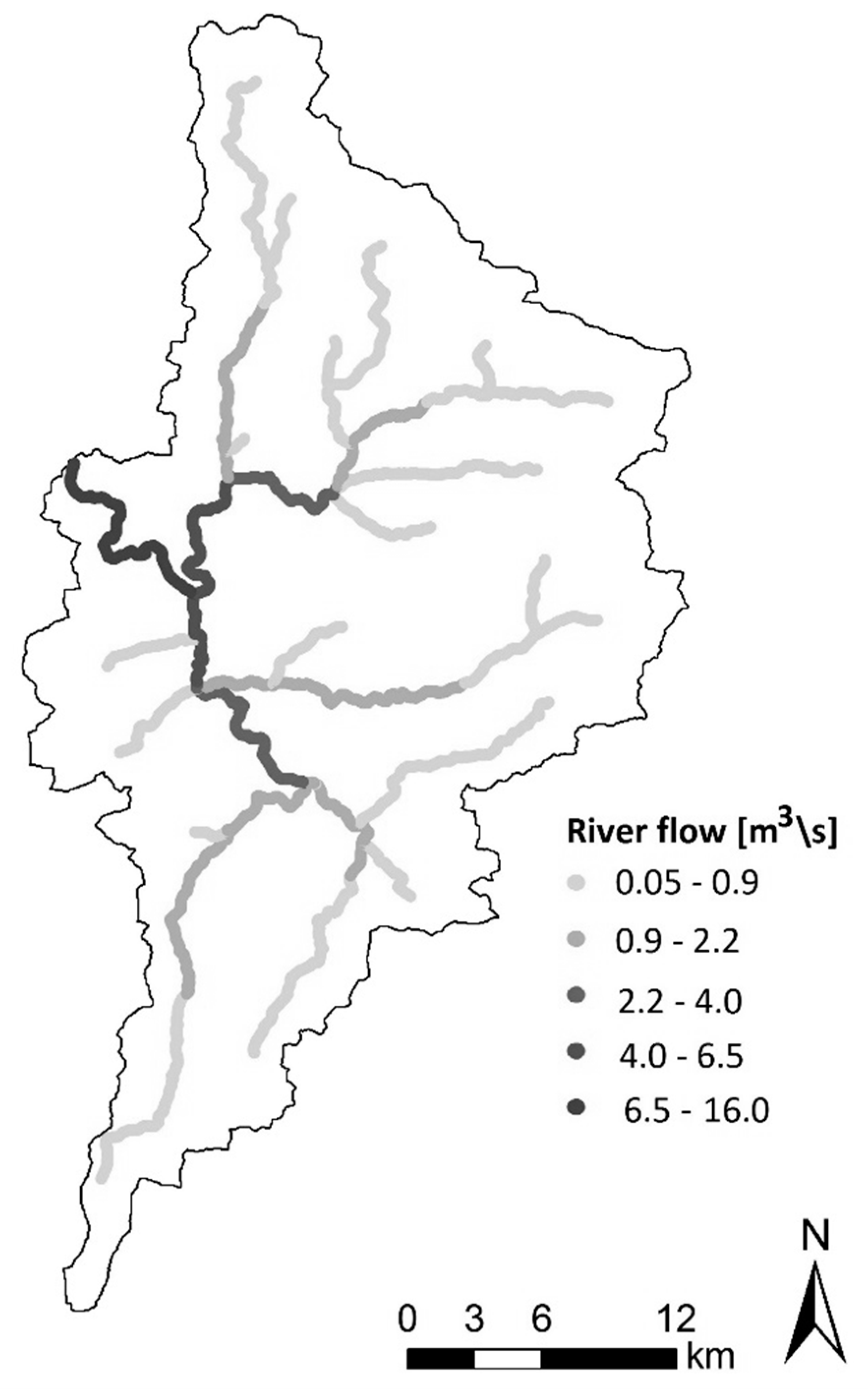
Once the model has been calibrated and validated, it has been applied to estimate daily river flow in each of the point selected according to the criteria that are described in Section 3.2. The simulated value of average annual river flow in each river channel is shown in Figure 7. In order 1 river channel, the average annual river flow ranges between 0.05 and 0.9 m³/s. The highest values of river flow are reached in the stream channel of order 4. 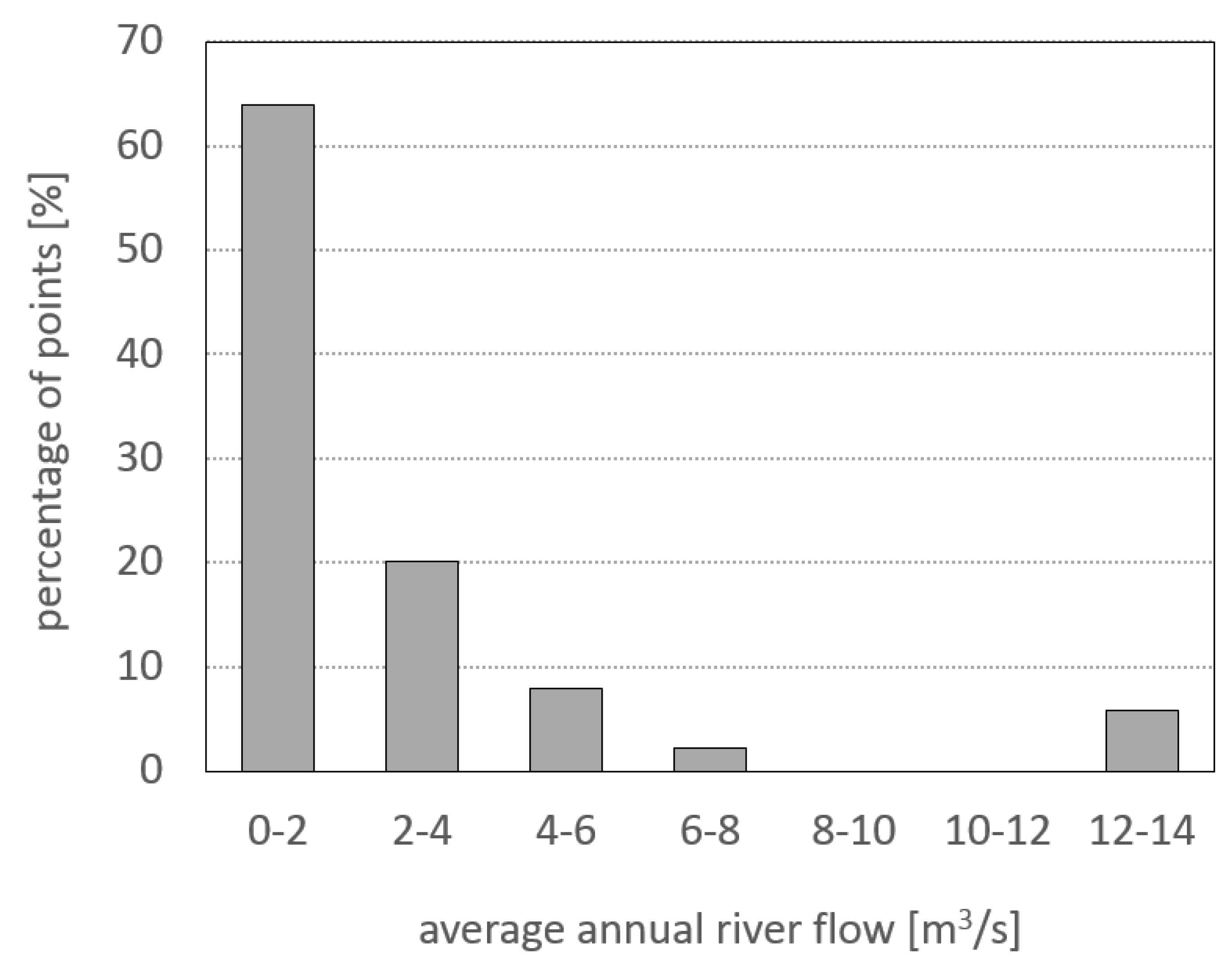Figure 8 shows the percentage of the analyzed points in each range of average annual river flow. In the 64% of the locations, the average annual river flow ranges between 0 and 2 m³/s. The highest values of average annual river flow can only be reached in the 6% of the analyzed sites. Starting from the simulated river flow series, the flow-duration curves have been assessed and used to identify the 50% and the 75% dependability river flow. For each of these river flow values, the potential hydropower has been calculated while using Equation (1).

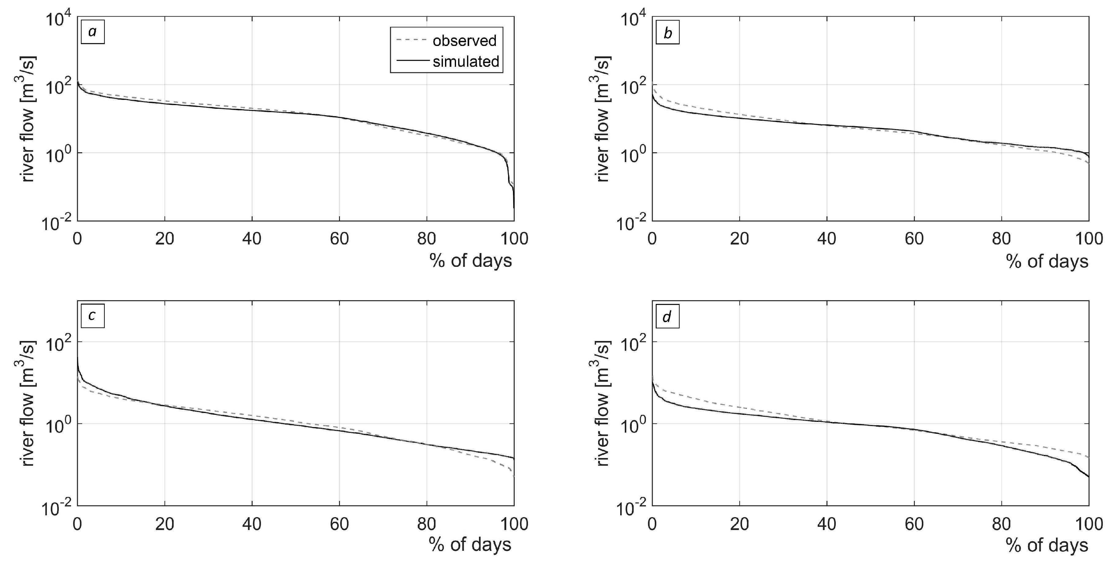
Figure 9 shows the flow-duration curves for the river basin outlet (outlet 50001) evaluated while using simulated data over the 2000–2006 period, and for the other locations for which daily river flow measurements were available (outlets 50006, 50007, and 50012). The comparison between the flow-duration curves that were obtained using simulated river flow shows a good agreement with those that were obtained using observed data. Specifically, the 50% and the 75% dependability river flow are well captured by the model, as reported in

Table 3. Comparison between 50% and 75% dependability river flow values evaluated from observed and simulated flow-duration curves for each outlet.

Outlet	50% Dependability		75% Dependability
	Observed	Simulated	Observed	Simulated
50001	15.78	14.47	4.22	5.02
50006	4.80	5.40	2.06	2.17
50007	0.92	1.10	0.38	0.37
50012	0.90	0.90	0.41	0.37

. These results point out that SWAT is able to provide reliable output not only for the outlet in which it has been calibrated, but also for outlet related to upstream sub-basins.

4.3. Hydropower Locations

The procedure required, as input data, the layer hydrographic network and the DEM. Firstly, the river network has been divided into equal segments of 100 m using the GIS tools. Successively, the head has been calculated for each point along the river network and the daily river flow has been evaluated by means of SWAT in each sub-basins in which the points are located. Once the head and the river flow have been assessed, the power has been calculated while using the Equation (1).

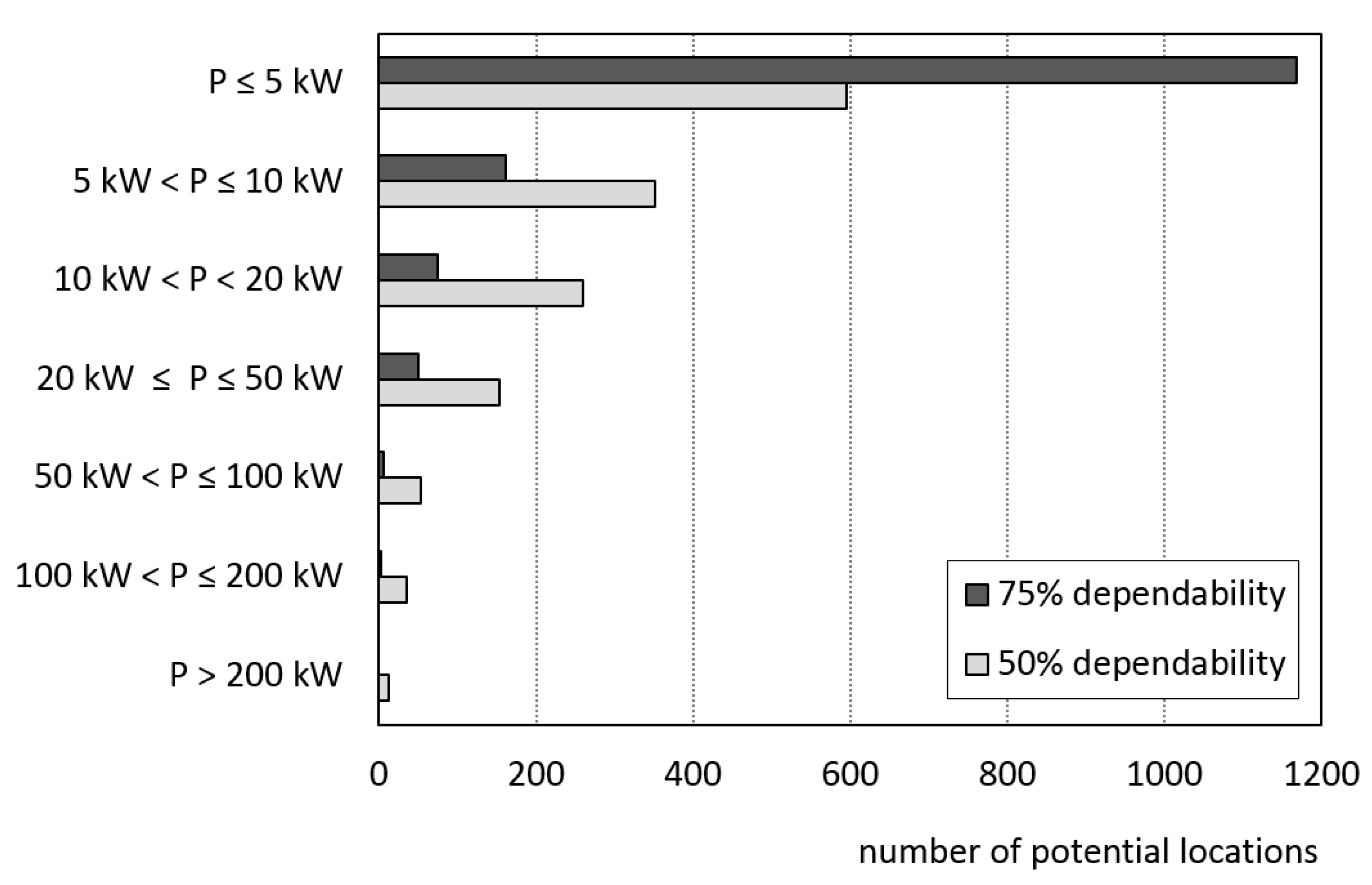
A total of 2189 locations along the river network has been analyzed using the proposed procedure (Figure 10). For each degree of dependability, the potential power of each site has been assessed. For the 50% dependability, the procedure identified 1463 potential locations. According to the results, the river network is more suitable for power plants of small size (P ≤ 50 kW), but greater hydropower plants (100 kW < P ≤ 200 kW) can be also installed (up to 50 sites). Specifically, approximately 600 locations that are distributed in almost all the reaches of the river could be chosen for plant installation with potential power up to 5 kW. For 20 kW ≤ P ≤ 50 kW, 50 kW < P ≤ 100 kW, and 100 kW < P ≤ 200 kW, respectively, 153, 51, and 36 locations resulted in being suitable. Only 13 locations have been found to be selectable for P > 200 kW. For the 75% dependability, 1169 sites have been found to be suitable for small plants (P ≤ 5 kW). Potential power ranging between 10 and 20 kW could be reached in 161 sites. For 20 kW ≤ P ≤ 50 kW and 50 kW < P ≤ 100 kW, respectively, 50 and six locations could be selected for the installation of hydropower plants. Higher values of power (100 kW < P ≤ 200 kW) can only be reached in three locations. A power greater than 200 kW cannot be reached in any of the analyzed locations.

In this study, only sites with a power greater than 20 kW have been taken into account. Specifically, the following ranges of power have been considered: 20 kW ≤ P ≤ 50 kW, 50 kW < P ≤ 100 kW, 100 kW < P ≤ 200 kW, and P > 200 kW.

For a 50% dependability degree, 256 sites have been identified as being suitable for run-of-river installation. Among these, the 61% of sites are included in the smallest power category (20 kW≤ P ≤ 50 kW). These plants can be generally positioned along all of the river network, but not everywhere: the channel reaches extremely far from the outlet section of the river basin seems to not be particularly suitable for this purpose. The 20% of sites fall in the 50 kW < P ≤100 kW range, while the 14% of sites are able to provide a potential hydropower in the 100 kW < P ≤ 200 kW range. The remaining 5% of sites can provide a potential power greater than 200 kW. Generally, the highest hydropower plants sites (P > 100 kW) fall close to the outlet section of the river basin, but some of these plants can be also placed far from the outlet section, where the flow rate is lower, but where remarkable drop heads sometimes occur.

For the 75% dependability, 59 locations could be selected for run-of-river plants. In this case, the 85% of potential sites are included in the smallest power category (20 kW ≤ P ≤ 50 kW). Most of them are located in reaches of third and fourth order. The 10% of sites fall in the 50 kW < P ≤ 100 kW range, while the remaining 5% of sites can provide potential power in the 100 kW < P ≤ 200 kW range. None of the analyzed sites is suitable for run-of-river plants with P > 200 kW. The potential sites for hydropower with the 75% dependability are located closer to the river basin outlet, if compared with the locations found for the 50% dependability.

For 50% and 75% dependability, as the runoff contributing area increase and, consequently, river flow, the number of sites increases from the upstream to downstream of the catchment. Even if the average slope and, thus, the head, tends to decrease from upstream to downstream, the downstream reaches of the river network provide a greater number of locations for hydropower installation.

It has to be remarked that the identification of potential sites described here only takes topographic and hydrological aspects into account. Once the potential locations have been detected, the environmental and economic feasibility of small hydropower plants in these sites has been assessed.

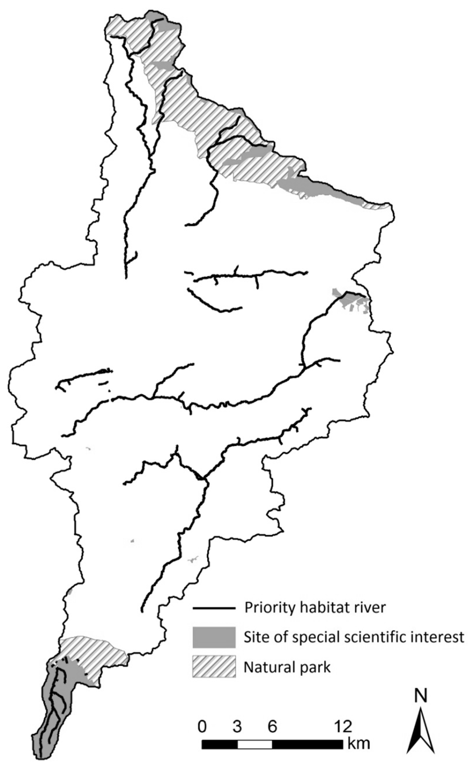
4.4. Environmental Analysis Results

The detected potential locations have been filtered out while using the exclusion layer that is shown in Figure 4. This procedure allowed for excluding from the sites those that are located in areas of high environmental sensitivities. For 50% dependability, the intersection of the potential hydropower sites with the exclusion layer led to the selection of 83 from the initial 253. Specifically, 170 locations have been excluded in the 20 kW ≤ P ≤ 50 kW power range, nine locations in the 50 kW < P ≤ 100 kW range, and just one location in the 100 kW < P ≤ 200 kW range. All of the potential sites with P > 200 kW were outside the protected areas. As regards to the 75% dependability, the environmental analysis only led to the exclusion of two sites in the 20 kW ≤ P ≤ 50 kW power range.

4.5. Economic Analysis Results

The potential locations that were obtained from the environmental analysis have been subjected to an economic analysis. One of the expressions suggested for the UK by Gallagher et al. [35] has been used in order to assess the turbine/generator costs. Gallagher et al. [35] proposed different formulas for the most common types of turbine. In this study, it has been assumed that the hydropower plants in the detected potential locations were equipped with Kaplan turbines. Indeed, these turbines have high efficiencies across medium and low heads, such as those that were detected for the area of study.

The following expression, valid for the 9–300 kW power range, has been used to calculate the turbine/generator costs C.

$$C=22155·P^{0.440}·H^{-0.152}$$

(6)

In this formula, power P has been multiplied by the efficiencies of the Kaplan turbine and the generator (0.9 and 0.9, respectively). The equation provides a quite accurate evaluation of the generator and turbine costs within a range of ±30%. The obtained costs have been increased of the 10% in order to take into account for the maintenance costs [26]. In the case of hydropower plants with a P smaller than 100 kW, the main contribution to the total costs is given by the cost of the turbine and generator. Therefore, the assessment of C by means of the Equation (6) can be considered to be reliable. Nevertheless, the report of the International Renewable Energy Agency points out that the cost of the turbine/generator unit considerably varies as a percentage of costs of the total project [39]. Thus, for values of P that are greater than 100 kW, the cost of civil works gives an important contribution to the total cost. In these cases, to get a more reliable estimate, the cost that was obtained by the Equation (6) has been increased of the 50%. Once C has been evaluated for each of the selected potential locations, the economic payback EP has been calculated while using Equation (5) and considering an income i from FITs equal to 0.09 €/kWh [40].

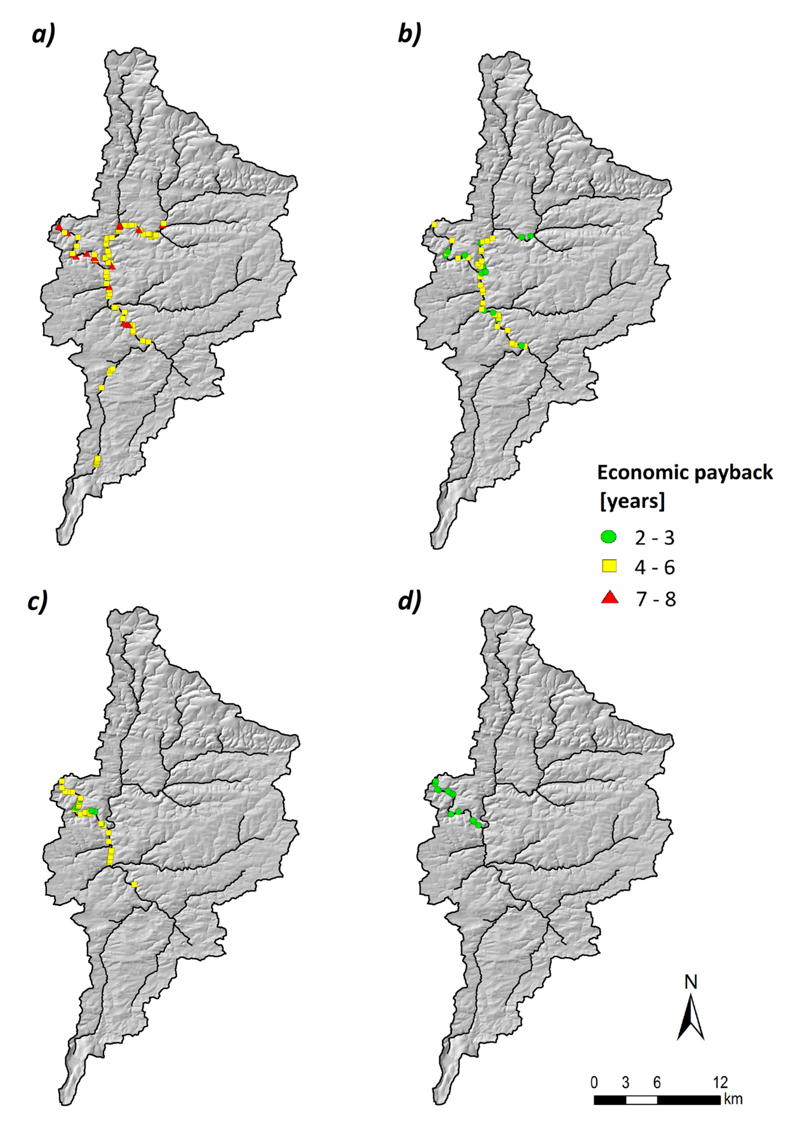
The EP values that were obtained for each potential locations have been reported in the maps in Figure 11 and Figure 12. For 50% dependability, 83 potential locations have been identified in the 20 kW ≤ P ≤ 50 kW power range (Figure 11a). For the 86% of these sites, the EP ranges from four to six years, whereas for the remaining 14% the EP varies between seven and eight years. For the 50 kW < P ≤ 100 kW power range, 42 sites are adequate for run-of-river plant installation (Figure 11b). For the 31% of these locations, the EP is between two and three years, while for the 69% of sites, the EP is between four and six years. For the 100 kW < P ≤ 200 kW power range, the EP is 4–6 years for the 91.5% of the cases (32 sites). Only three locations provided a higher EP (Figure 11c). Figure 11d shows that, for P > 200 kW, in all 13 potential locations, hydropower plants with EP ranging from two and three years could be installed.

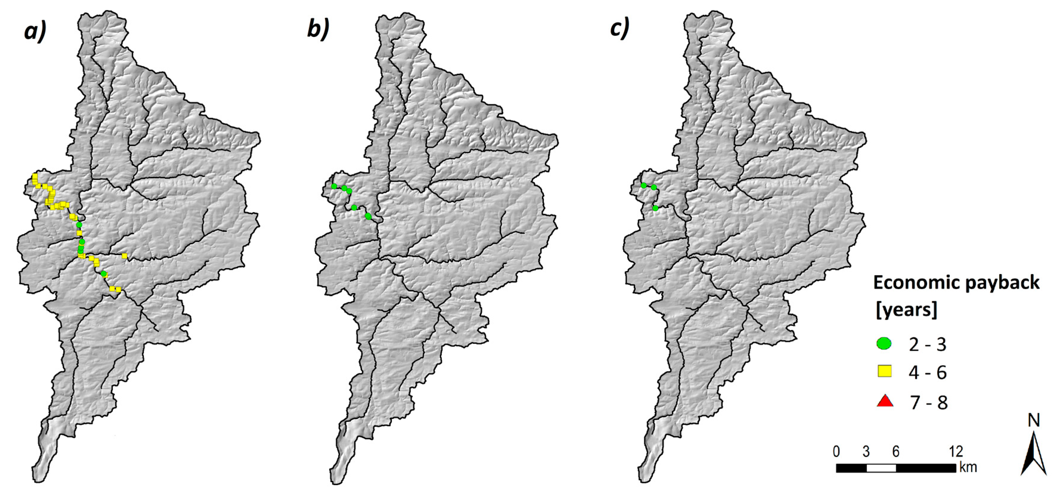
For 75% dependability, 48 sites have been selected for the installation of hydropower plants with 20 kW ≤ P ≤ 50 kW. The 73% of these sites are suitable to install hydropower plants with EP that ranges between four and six years. Smaller EPs (2–3 years) have been assessed for the remaining 27% of locations (Figure 12a). For the 50 kW < P ≤ 100 kW power range, six potential sites have been identified (Figure 12b), for which the EP is 2–3 years. Only three sites (all with EP between two and three years) are adequate for hydropower plants with 100 kW < P ≤ 200 kW (Figure 12c). No sites are suitable for installation with P > 200 kW.

5. Conclusions

Small hydroelectric plants represent a reliable cost-effective electricity supply, which is based on a renewable and sustainable resource. In this study, different methodologies and analysis, available in literature, have been combined to provide a screening procedure that is useful for performing a preliminary analysis for the detection of potential run-of-river plant locations. Specifically, GIS tools and the SWAT model have been employed to identify potential hydropower sites in the Taw at Umberleigh, a large rural catchment located in South West England. The inclusion of the environmental and economic analysis in the procedure allowed for excluding all of the potential locations that are suitable in terms of river flow and head, but they have environmental issues or are not cost-effective.

Calibration and validation of SWAT for the above-mentioned catchment showed that the model is able to provide a reliable estimation of the river flow.

The potential locations that were detected while using GIS tools and the SWAT model have been successively analyzed in order to evaluate the environmental and economic feasibility of small hydropower plants in these sites. The results have been summarized in some maps that show the locations of potential hydropower sites for different power thresholds and the related economic payback period for turbine and generator. A great number of sites has been identified for each threshold, therefore the application of the procedure pointed out the high potential of the area in terms of hydropower exploitation.

The procedure is valid and easy to apply to different cases of studies. The used GIS tools are available in open source softwares, while SWAT is a public domain model that can be applied by means of one of its open source GIS interfaces. Obviously, equations for the calculation of the economic payback valid for the area of interest need to be specifically defined or, if possible, found in the literature.

It has to be remarked that results that were obtained by the application of the GIS-based procedure can be considered to be an effective support for preliminary or pre-feasibility studies in hydropower planning. The accuracy of DEM has important implications in the identification of potential run-of-river locations. The OS Terrain 50 grid used in this study has been verified to provide a Route Mean Square Error (RMSE) of 4 m. DEM quality affects the river network delineation procedure in SWAT. For these reasons, field measurements are required to verify the reliability of the identified locations. Additionally, the economic feasibility of the run-of-river plant needs to be investigated with at-site surveying for every single case. Moreover, the installation of various small plants along the same river channel requires a more accurate planning, in order to limit the implications of the water intake on the hydrological and ecological characteristics of the river. Indeed, the water diversion can affect the river regime and it have consequences on the downstream habitat conditions for the riverine biodiversity. Nevertheless, environmental impact issues, such as those that are related to water oxygenation and downstream erosion, can be mitigated by using proper design techniques.

In summary, the methodology here proposed could be a valuable support for decision-makers in the preliminary identification of the most suitable locations to install run-of-river plants in the area of study. Moreover, the evaluation of the economic payback allows for the selection of the sites for which the economic investment is more affordable. However, for each case, an at-site surveying cannot be avoided, since the feasibility of the hydropower plant needs to be confirmed by data that were collected in the field. Indeed, the topographic, hydrological, and environmental characteristics of each site are unique, therefore the installation of run-of-river plants can require different technical solutions every time.