Abstract
Incipient faults in power cables are a serious threat to power safety and are difficult to accurately identify. The traditional pattern recognition method based on feature extraction and feature selection has strong subjectivity. If the key feature information cannot be extracted accurately, the recognition accuracy will directly decrease. To accurately identify incipient faults in power cables, this paper combines a sparse autoencoder and a deep belief network to form a deep neural network, which relies on the powerful learning ability of the neural network to classify and identify various cable fault signals, without requiring preprocessing operations for the fault signals. The experimental results demonstrate that the proposed approach can effectively identify cable incipient faults from other disturbances with a similar overcurrent phenomenon and has a higher recognition accuracy and reliability than the traditional pattern recognition method.
1. Introduction
As a crucial link in power systems, power cable failures are bound to cause substantial losses for power companies and residents. Various methods have been proposed to reduce the occurrence of cable faults. In [1], power cable faults are divided into three stages: cable defects [2], incipient faults [3], and permanent faults. Cable defects, caused by environmental stress, mechanical stress and other influences, become incipient faults with the enhancement of the partial discharge, and over time, incipient faults repeatedly occur and eventually develop into permanent faults. Incipient faults can usually be identified by overcurrent signals. However, interference signals, such as transformer inrush and capacitor switching, also display overcurrent characteristics, which makes it difficult to accurately identify incipient faults in power cables. If an incipient fault in a power cable can be identified in time and targeted maintenance can be performed, a permanent fault can be avoided. Therefore, it is of great practical significance to accurately identify incipient faults in power cables.
Currently, traditional pattern recognition and deep neural networks (DNN) are mainly used to recognize incipient faults in power cables. This traditional recognition method includes three key steps: data preprocessing, feature extraction, and fault recognition. First, dimensionality reduction processing is carried out on the original data through principal component analysis [4] and other methods. Then, feature extraction is carried out on the data through a wavelet transform (WT) [5] and other time-frequency domain processing methods. Finally, the extracted features are classified through the use of a support vector machine (SVM) [6] and other classification methods. In [7], using the wavelet decomposition of current signals, Sidhu, T. S. et al. determine whether there is an incipient fault based on the energy and the root mean square (RMS) contrast threshold. However, the results show that this method is less robust and leads to a higher false detection rate. Zhang, W. et al. [8] detect the fault signal and calculate a new signal by using a Kalman filter to determine whether there is an incipient fault. In [9], it is assumed that the incipient cable fault is an arc fault, and the harmonic distortion rate of the fault voltage is calculated to determine whether an incipient fault occurs by comparing the distortion rate to the reference threshold. In general, when the assumed conditions are inconsistent with the actual operating conditions, the above methods will not be able to accurately identify the incipient fault. With the development of artificial intelligence, methods for incipient fault identification based on neural networks have appeared [10]. As in [1], the characteristic quantities, such as energy entropy and singular entropy, of the decomposed signal after S transformation are artificially extracted to serve as the input for a stacked autoencoder to recognize incipient faults. Ebron, S. et al. [11] trained a neural network to detect high-impedance faults. The advantage of this neural network method is that it can autonomously learn the required feature information from the current signal, and avoid the problem of the feature loss caused by artificial feature extraction. However, most neural networks use preprocessed features as an input; which is mainly restricted by the overfitting of the deep neural network during training, the easy convergence to local optimal solutions, the slow convergence speed, and other problems [12,13,14]. The application of deep neural networks was not possible until Hinton, G.E. et al. [15] proposed their revolutionary deep learning theory. Deep learning technology has been widely applied for motion recognition [16], semantic understanding [17], mechanical fault diagnosis [18] and other fields, resulting in remarkable achievements, but its application to fields related to power systems [19] has been very limited.
In this paper, a sparse autoencoder is combined with a deep brief network to build a deep neural network. The problems in the learning process of the deep neural network are overcome by determining the network’s parameters through the deep learning method of layer-by-layer greedy unsupervised pretraining. The network weight is further optimized through supervised reverse fine-tuning, and incipient faults can be identified quickly and accurately in multiple cable overcurrent disturbances, i.e., transformer inrush, capacitor switching, and constant impedance failure. The algorithm structure is shown in Figure 1.
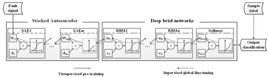
Figure 1.
Structure diagram of the algorithm.
2. Methods
The traditional fault identification methods are largely dependent on feature extraction and feature selection, which require professional knowledge in the field of signal processing. A deep neural network with multiple hidden layers has strong feature learning ability and can automatically learn feature information from massive amounts of data, avoid the subjectivity caused by artificial feature extraction and identify incipient faults in power cables. Commonly used deep neural network structures include stacked autoencoders [20], deep brief networks [21] and convolutional neural networks [22]. In this paper, a sparse autoencoder and deep brief networks are cascaded to build deep neural networks. The data from the nonlinear transformation of the sparse autoencoder are fed into the deep brief networks in a more compact form. Then, the implicit features learned in the deep brief networks are fed into a Softmax [23] classifier to recognize incipient cable faults. This network structure not only overcomes the problems of the heavy load and high computational complexity of the traditional neural networks but also overcomes the problem of the poor performance of deep brief networks when processing large amounts of data [24].
2.1. Sparse Autoencoder
The structure of the autoencoder (AE), as shown in Figure 2, is a symmetrical network structure composed of three layers of neurons: an input layer, a hidden layer, and an output layer.
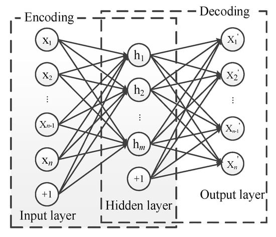
Figure 2.
Structure of autoencoder.
The AE tries to obtain the approximate value of the input in the hidden layer to perfectly reproduce the input in the output layer. The neurons in the first two layers complete the encoding process, and the last two layers complete the decoding process. With the help of the back-propagation algorithm [25], most of the core characteristics of the input data are learned in an unsupervised manner by minimizing the reconstruction error. The encoding and decoding processes can be represented as follows:
where, and are the activation functions of each layer, and are the input and output units, is the hidden unit, and are the weight matrices between the neurons of each layer, and , are the biases of each layer.
Although AE can perfectly reproduce the input data in the output, the AE does not effectively extract meaningful features by simply copying the input layer to the hidden layer. The sparse autoencoder (SAE), as an extension of the AE, causes the AE to learn relatively sparse [26] features by introducing a sparsity constraint. Sparsity refers to the property that most neurons in the hidden layer of the AE are in a suppressed state. In the experiment, the activation function , namely, a sigmoid function, maps the output to the interval (0, 1). Therefore, when the output of the hidden layer is close to zero, it is regarded as in an inhibitory state, and the construction of the SAE is achieved when sparsity restrictions are imposed on the AE and most hidden layer nodes are in an inhibitory state. This condition can improve the performance of the traditional AEs and make them more practical.
Since the output reproduces the input, the mean square error is used to construct the loss function, as shown in Equation (3), and the unsupervised training on the SAE is conducted by minimizing the loss function.
To achieve the sparsity limitation, the average activation degree of the i-th neuron in the hidden layer is defined as
In the formula, n represents the number of neurons in the input layer. To make the activation degree of most neurons in the hidden layer tend to zero, a sparse parameter close to zero is introduced, with = . Meanwhile, a penalty factor is introduced based on the relative entropy shown in Equation (5) to discount cases with a large difference between and .
The penalty factor increases with the difference between and , and the value is zero when = . The total loss function for the SAE is then obtained as
where m represents the number of neurons in the hidden layer and the network weight coefficients W and b are obtained by minimizing the loss function to obtain the optimal expression for the input data. The SAE can reduce the dimension of complex signals without feature loss.
2.2. Deep Brief Networks
A deep brief network (DBN) is a probability generation model developed based on biological neural networks. The DBN infers the sample distribution for the input data according to the joint probability distribution. By adjusting the weight coefficient between the network layers, the entire network can generate implicit feature data with maximum probability. Commonly, the DBN is made up of a restricted Boltzmann machine (RBM) and a classifier.
2.2.1. Restricted Boltzmann Machine
As the core component of the DBN, an RBM is a probabilistic model based on an energy function [27], that can learn relationships and rules in complex data in an unsupervised way. An RBM is a two-layer recursive neural network composed of a hidden layer and an explicit layer, as shown in Figure 3.
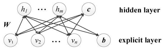
Figure 3.
Structure of restricted Boltzmann machine.
The interlayer neurons of the RBM adopt bidirectional full connections, while there are no connections within a layer, which ensures the conditional independence between each layer. That is, for a given explicit element, the implicit element values are not correlated with each other, and the explicit element values are not correlated with each other when an implicit element is given, thus reducing the operational complexity of the whole network and improving the training speed.
An RBM makes the probability distribution of the output as close as possible to the probability distribution of the input through unsupervised training. As a typical probability generation model, the RBM uses the probability distribution of samples to obtain a high-level representation of the features. For a given state (v, h), the energy functions of the RBM can be defined as
where = {w, b, c} represents model parameters, represents the state and bias of the explicit element, represents the state and bias of the hidden element, represents the weight coefficient between the i-th explicit element and the j-th implicit element. The state probability distribution of an RBM obeys a regular distribution, so the joint probability distribution for the state (v, h) is , where is the normalized factor. According to the interlayer conditional independence, when the status of the explicit layer is determined, the activation probability of the j-th hidden layer neuron is
where f(x) is the activation function, and when the hidden layer unit is determined, the activation probability of the i-th explicit layer neuron is
For the training sample set S ={}, where is the number of training samples, the training objective is to maximize the likelihood function to obtain the model parameter .
To complete the training of an RBM, it is necessary to calculate the negative gradient of the logarithmic likelihood for its parameters and solve for all the possible values of the corresponding v and h, which introduces great operational complexity and reduces the learning efficiency of the network. In practice, we train the network by using a contrastive divergence (CD) algorithm [28]. The CD algorithm greatly improves the learning efficiency of an RBM and the performance of the entire neural network. Through the batch processing of the training data, the training speed of the network is further improved.
2.2.2. Softmax Classifier
To achieve fault recognition in a DBN, a classifier is also an essential component. In this experiment, multiple types of faults need to be recognized. Therefore, a Softmax classifier and an RBM are selected to build the deep brief networks. Unlike the traditional binary classifier, a Softmax classifier is more suitable for the classification of multiple mutually exclusive events. The activation function of the Softmax classifier is , and it maps the output of multiple neurons to the interval (0, 1) and takes the resulting probability as the classification basis to achieve the classification of multiple events. The output of the classifier is
where K is the total number of categories. A Softmax classifier is a supervised neural network. By combining the outputs with sample tags to achieve the supervised training of the network, the back-propagation algorithm is used to perform global fine tuning for the whole neural network and complete the training of the deep neural network.
2.3. Fault Identification Based on Deep Neural Network
The deep neural network is composed of an SAE and a DBN. The training of the whole network is achieved through two steps of layer-by-layer unsupervised greedy pretraining and reverse supervised fine-tuning, to determine the weight coefficient between the neurons in each layer. The pretraining of the SAE and the DBN alone can only ensure that the internal weights of the network can achieve the best mapping of the characteristics of the layers. To ensure the overall performance of the deep neural network, the global fine-tuning of the network parameters through supervised training is essential. In this paper, a deep neural network is built to identify incipient faults in power cables with its powerful feature learning ability. The complete algorithm flow chart is shown in Figure 4.
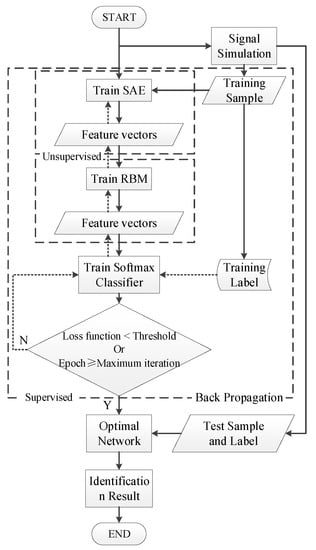
Figure 4.
Flowchart of the proposed algorithm.
The identification process can be summarized in the following five steps:
- Data preprocessing: divide the required samples into two parts, namely, the training set and the test set, and make the sample labels according to the fault categories;
- Network initialization: set the initial state of the network from experience, debug and determine the number of network layers, the number of nodes, and the number of training iterations;
- Network pretraining: the SAE and the DBN are constructed through layer-by-layer unsupervised training, and the network weight coefficients of each layer are determined;
- Back propagation global fine-tuning: reconstructed features are fed into the classifier, and a back-propagation algorithm is applied to complete the supervised training of the deep neural network and the fine-tuning of the network parameters;
- Fault identification test: the test data are sent to the trained deep neural network for sample tag classification and identification, and the network identification accuracy is verified according to the output identification results.
3. Results
3.1. Construction of the Sample Data Set
To evaluate the performance of the proposed identification method, a cable line model [9] for a 60 Hz power system is constructed in a PSCAD/EMTDC, as shown in Figure 5. represents the model voltage source, is the cable voltage drop, is the fault point voltage, is the bus voltage, is the cable voltage, is the feeder current, is the system impedance, is the load impedance.
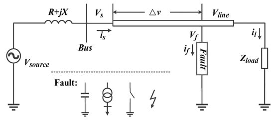
Figure 5.
Model of a cable line.
To make the simulation process more similar to the case of a fault in a grid system, we simulated subcycle and multicycle (general lasts for 1–4 cycles) incipient cable faults, three overcurrent disturbance signals and a normal current signal to be identified. The overcurrent signals are generated by an IEEE 13-node test system [29], and the corresponding current waveforms sampled at a 10 kHz sampling rate are shown in Figure 6.
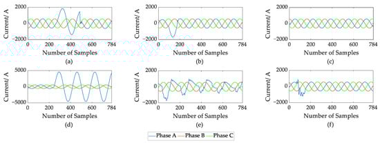
Figure 6.
Current waveform for a cable fault: (a) Multicycle incipient fault; (b) Subcycle incipient fault; (c) Normal signal; (d) Constant impedance failure; (e) Transformer inrush disturbance; (f) Capacitor switching disturbance.
The simulation obtained a total of 16,800 samples in six categories, including 2100 training samples in each category and 700 test samples, and made corresponding classification labels. The failures in the five categories were all guaranteed not to occur at the same time and (10, 20, 30, 40, 50, 60, 70, 80) dB white noise was added to the signals in the simulation process as a comparison to simulate actual fault conditions.
In the experiment, the prediction accuracy is used to evaluate the effectiveness of the DNN and the recall rate is used to evaluate the recognition performance of various signals. The accuracy represents the percentage of correctly identified samples in all samples. While the recall rate (or true positive rate) represents the percentage of the samples that were correctly identified as a certain type in all samples of this type [30].
3.2. Establishment and Training of the DNN
To identify incipient faults in power cables, the neural network needs to be trained with training samples. Good results can be obtained by selecting appropriate network parameters and interlayer connection weight coefficients.
3.2.1. Initialization of DNN
To build a neural network, the number of neural network layers and the number of neurons contained in each layer of the network should be determined first. We select the number of layers according to the results in Table 1.

Table 1.
Recognition performance of different network structures.
After many experiments, according to the recognition accuracy and the recall rate under different network structures, we determined the number of hidden layers in the SAE and that in the DBN is (1–2).
The initial network parameters are selected based on experience, and the fault identification accuracy under different numbers of neurons contained in each layer is tested, as shown in Figure 7. The classification accuracy is the best when the network structure is (784-60-100-40-6), where 784 and 6 denote the numbers of input and output neurons, respectively, 60 and {100, 40} denote the neuron numbers of the hidden layers in the SAE and the DBN. Accordingly, the structure of the deep neural network established in the experiment is shown in Figure 8.
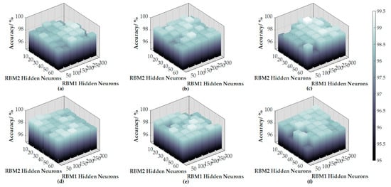
Figure 7.
Identification performance for different network structures: (a) 20 hidden neurons in an sparse autoencoder (SAE); (b) 40 hidden neurons in an SAE; (c) 60 hidden neurons in an SAE; (d) 80 hidden neurons in an SAE; (e) 100 hidden neurons in an SAE; (f) 120 hidden neurons in an SAE.
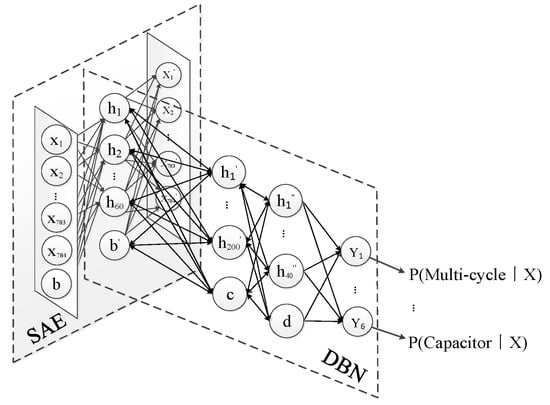
Figure 8.
Structure of deep neural network.
Based on this observation, layer-by-layer pretraining is carried out for each layer of the neural network.
3.2.2. Pretraining of the SAE and the DBN
The classification accuracy of the deep neural network is tested at different learning rates and different epochs of the SAE, the results are shown in Figure 9a. The learning rate and the minimum epochs required to achieve the best reproduction effect in the network were determined to achieve the best effect in the shortest time for the entire network. After many experiments, it is verified that the network performance can reach the best level after 100 iterations of training when the learning rate of the SAE is 0.4. Meanwhile, the interlayer weight coefficient was determined to provide a basis for weight initialization for the deep neural network.
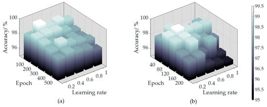
Figure 9.
Parameter adjustment: (a) Parameter adjustment of the SAE; (b) Parameter adjustment of the restricted Boltzmann machine (RBM).
Similarly, for the RBMs, as shown in Figure 9b, through multiple experiments, it is determined that 80 iterations of training can achieve the best network performance when the learning rate of the RBMs is 0.4, and the extracted feature vectors are sent to the classifier to achieve classifier pretraining.
3.2.3. Global Fine-Tuning
The pretraining of the classifier is completed by adding training tags, and the errors from the supervised training are transmitted back to the whole network from top to bottom to further optimize the parameters of each layer. We adjust the maximum epochs for the classifier and the deep neural network as shown in Figure 10. It is determined that the Softmax classifier achieves the best performance after 1020 iterations of training, while the DNN needs another 2300 iterations of training to achieve the best overall network performance.
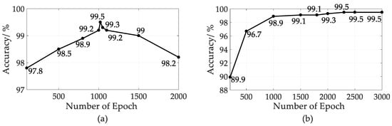
Figure 10.
Maximum epochs adjustment: (a) Epochs of Softmax Layer; (b) Epochs of deep neural networks (DNN).
After global fine-tuning, the whole deep neural network has both the rapidity of unsupervised training and the accuracy of supervised training.
3.3. Performance of the DNN
A total of 4200 test samples from 6 categories were sent to the trained deep neural networks for recognition, and the performance is shown as the confusion matrix in Figure 11.
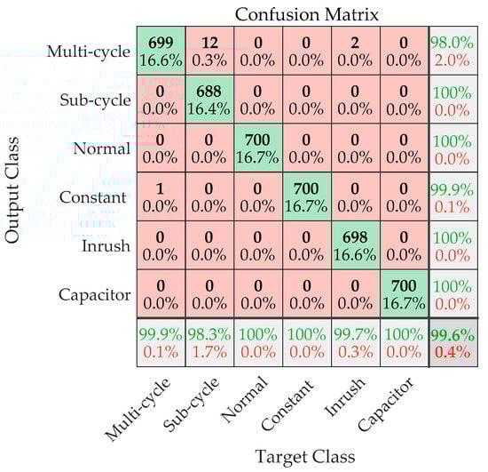
Figure 11.
Identification performance of the DNN.
In the confusion matrix, the rows correspond to the predicted class (output class), and the columns correspond to the true class (target class). The diagonal cells correspond to correctly classified observations, while the off-diagonal cells correspond to incorrectly classified observations. Both the number of observations and the percentage of the total number (4200) of observations are shown in each cell. The column on the far right of the plot shows the percentages of all the examples predicted to belong to each class that are correctly and incorrectly classified. These metrics are often called the precision (or positive predictive value) and false discovery rate, respectively. The row at the bottom of the plot shows the recall rate and false negative rate, and the cell at the bottom right of the plot shows the overall accuracy.
After adding 60, 40, and 20 dB white noise to the simulation signals, the identification accuracy (the results in the table have been cross-verified) of the proposed method for two types of incipient fault is shown in Table 2.
Table 2.
Recognition performance for incipient faults.
Furthermore, the two types of fault are combined as incipient faults. Statistically speaking, the identification accuracy of the proposed method for incipient faults under conditions of interference from various overcurrent signals reaches 99.8%. Similarly, after adding 60, 40 and 20 dB of white noise into the simulation signal, the accuracy is 99.8%, 99.7%, and 99.5%. Thus, the accuracy and effectiveness of this method for incipient fault identification are verified, which lays a foundation for its application in practice.
4. Analysis and Discussion
To verify the effectiveness of the deep neural network utilized in this paper, the traditional classification method and the shallow neural network identification method are compared with this method. In the experiment, the simulation configuration of the computer is as follows. OS: Windows 10 (64 bit); CPU: Inter(R) Core i7-8700 K (3.7 GHz), RAM: 16.0 GB; the version of MATLAB: 2016 b.
Similar to the above experiments, six types of signals, i.e., a normal current, a subcycle/multicycle incipient fault overcurrent signal and a transformer inrush overcurrent signal, were identified in the comparison experiments. Thus, in practical application, in addition to detecting the incipient faults in cables, other over current disturbance signals can also be identified.
Table 3 shows the overall identification accuracy and computational time of the method in this paper (SAE-DBN) compared with the traditional SVM and k-nearest neighbor (KNN) classifiers for the identification of the six types of signals. The comparison results show that the proposed method is superior to the SVM classifier in both the identification accuracy and speed. Although the KNN classifier has a fast identification speed, its classification accuracy is difficult to improve, so it cannot guarantee electrical safety.
Table 3.
Comparison of identification performance between our method and traditional classifiers.
Then, the proposed method is compared with four shallow neural network methods, e.g., SAE and CNN. Where, the CNN adopts lente-5 model [31] and adopts the form of 28 × 28 sample points as input. The overall recognition accuracies of the five methods are shown in Table 4, and the convergence rate for the proposed method compared with the other shallow neural networks is shown in Figure 12. In the experiment, the cross entropy is used as the loss function to train the neural networks. By analyzing the data in Table 4 and Figure 12, it is not difficult to find that, compared with shallow networks, the method in this paper has a faster identification speed and higher identification accuracy. The convergence rate for the neural network is greatly improved, and the local optimal solutions are avoided in the training process of the DNN. The performance is improved and the role of the SAE and the DBN in the deep neural network is verified. It also proves that the method in this paper can maintain a high accuracy under the premise of meeting the real-time [32] requirement of power systems.
Table 4.
Comparison of identification performance between our method and shallow networks.
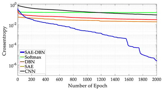
Figure 12.
Comparison of network convergence rate.
In this paper, simulation signals are directly used as an input to identify incipient faults and there is no need to carry out preprocessing steps, such as feature extraction, for simulated signals. The strong learning ability of the SAE and DBN networks is used to reconstruct and reduce the dimensionality of the input. The method in this paper is compared with the feature extraction of fault signals using the wavelet transform and classification by other classifiers. In the experiment, the db4 wavelet was used to carry out 8-layer wavelet decomposition on the original data, where each layer extracts 8 characteristics of the original signal, including the energy, mean value, variance, RMS value, Crest peak factor, skewness, kurtosis and information entropy. A total of 72 characteristic quantities are extracted and fed into the classifier for recognition and the results are shown in Table 5.
Table 5.
Comparison of the performance between our method and feature extraction method.
The experimental results show that the wavelet transform, as the most commonly used signal processing method, significantly reduces the noise in fault signals. In the case of large noise signals, the recognition accuracy of the classifier is effectively improved. However, when the noise signal is small, the recognition accuracy is reduced due to the loss of feature detail in the process of feature extraction. On the other hand, the feature extraction process greatly reduces the complexity of the samples to be classified, thus improving the recognition speed of the classifier. The comparison results also verify that the SEA and DBN networks provide good anti-noise capability and give the DNN a superior reproduction effect in the process of feature dimension reduction, thus avoiding the problem of feature loss.
In the power system, there are often various sources of signal interference, so the robustness of the identification method is important. Figure 13 shows the influence of various identification methods after adding (10, 20, 30, 40, 50, 60, 70, 80) dB white noise into the simulation signals. It can be seen that the performance of the method in this paper is superior to other identification methods regardless of the intensity of the noise. When the noise intensity reaches 20 dB, the recognition accuracy can be maintained at more than 95%, and when the noise intensity reaches 10 dB, the identification accuracy can still be maintained at more than 90%, which proves that the method in this paper is very robust and has broad application prospects.
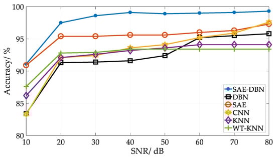
Figure 13.
The performance of different recognition methods under noise interference.
5. Conclusions
In this paper, an SAE and a DBN are combined to build a deep neural network for incipient fault identification in power cables. The simulation results show that this method can quickly and effectively identify incipient faults in power cables and has a high identification accuracy and robustness. Compared with other fault identification methods, it has the following advantages:
- Neurons in the hidden layer of the DNN can learn the high-order correlation of the input data and the most effective feature expression, and the problem of the feature loss caused by the subjective feature selection in traditional feature extraction is solved. The method in this paper can identify the incipient faults more accurately, thus avoiding permanent faults, as much as possible;
- Through unsupervised learning, the parameters of the whole neural network are preprocessed well, which solves the problems of overfitting, easy convergence to local optimal solutions and a slow convergence speed in the identification process. It improves the reliability and recognition speed of the algorithm and makes it more practical;
- The network is used to identify incipient faults in power cables, and the original fault signal is directly taken as the input. A well-trained DNN can complete the identification of a single fault signal within 0.0005 s, which greatly improves the real-time performance of the fault identification. On the other hand, no operator is required to have professional knowledge in the time-frequency field, which makes this method easier to use and more suitable for the production process; and
- The DNN adaptively extracts the most effective features in the original signal and identifies faults. The DNN simplifies the operation and makes the identification process more flexible, which makes it possible for the method to be applied in more fields.
On the other hand, since the method in this paper completely relies on the DNN to identify the incipient faults in power cables, the identification performance largely depends on the accuracy and integrity of the fault samples and the corresponding labels. Compared with the traditional fault identification method, the method in this paper needs more fault samples to fully train the DNN model in order to get better identification performance. At the same time, DNN lacks interpretability, and the basis for fault identification is not as obvious as traditional methods.
This paper proposes the application of a DNN to incipient fault identification in power cables, which provides a new idea for research in this field. After practical engineering verification, this method will be widely used.
Author Contributions
Software, N.L.; Investigation, B.F.; Methodology, X.X. and X.Y.
Funding
This research received no external funding.
Conflicts of Interest
The authors declare no conflict of interest.
References
- Wang, Y.; Lu, H.; Yang, X.M.; Xiao, X.; Zhang, W. Cable incipient fault identification based on stacked autoencoder and S-transform. Electr. Power Autom. Equip. 2018, 292, 124–131. [Google Scholar]
- Fengyuan, Y.A.N.G.; Yongpeng, X.U.; Xinlong, Z.H.E.N.G. Partial discharge pattern recognition of HVDC cable based on compressive sensing. High Volt. Eng. 2017, 43, 446–452. [Google Scholar]
- Kojovic, L.A., Jr.; Williams, C.W. Sub-cycle detection of incipient cable splice faults to prevent cable damage. In Proceedings of the IEEE Power Engineering Society Summer Meeting, Seattle, WA, USA, 16–20 July 2000; Volumes 1–4, pp. 1175–1180. [Google Scholar]
- Xu, L.; Tan, C.; Li, X.; Cheng, Y.; Li, X. Fuel-Type Identification Using Joint Probability Density Arbiter and Soft-Computing Techniques. IEEE Trans. Instrum. Meas. 2012, 61, 286–296. [Google Scholar] [CrossRef]
- Bhattacharyya, A.; Pachori, R.B.; Acharya, U.R. Tunable-Q Wavelet Transform Based Multivariate Sub-Band Fuzzy Entropy with Application to Focal EEG Signal Analysis. Entropy 2017, 19, 99. [Google Scholar] [CrossRef]
- Moualeu, A.; Gallagher, W.; Ueda, J. Support Vector Machine classification of muscle cocontraction to improve physical human-robot interaction. In Proceedings of the IEEE/RSJ International Conference on Intelligent Robots & Systems, Chicago, IL, USA, 14–18 September 2014; pp. 2154–2159. [Google Scholar]
- Sidhu, T.S.; Xu, Z. Detection of Incipient Faults in Distribution Underground Cables. IEEE Trans. Power Deliv. 2010, 25, 1363–1371. [Google Scholar] [CrossRef]
- Ghanbari, T. Kalman filter based incipient fault detection method for underground cables. IET Gener. Transm. Distrib. 2015, 9, 1988–1997. [Google Scholar] [CrossRef]
- Zhang, W.; Xiao, X.; Zhou, K.; Xu, W.; Jing, Y. Multi-Cycle Incipient Fault Detection and Location for Medium Voltage Underground Cable. IEEE Trans. Power Deliv. 2016, 32, 1450–1459. [Google Scholar] [CrossRef]
- Voumvoulakis, E.M.; Gavoyiannis, A.E.; Hatziargyriou, N.D. Application of Machine Learning on Power System Dynamic Security Assessment. In Proceedings of the International Conference on Intelligent Systems Applications to Power Systems, Toki Messe, Niigata, Japan, 5–8 November 2007; pp. 1–6. [Google Scholar]
- Ebron, S.; Lubkeman, D.; White, M. A neural network approach to the detection of incipient faults on power distribution feeders. IEEE Trans. Power Deliv. 1990, 5, 905–914. [Google Scholar] [CrossRef]
- Van Schaik, N.; Czaszejko, T. Conditions of discharge-free operation of XLPE insulated power cable systems. IEEE Trans. Dielectr. Electr. Insul. 2008, 15, 1120–1130. [Google Scholar] [CrossRef]
- Zhang, S.; Wang, Y.; Liu, M. Data-based Line Trip Fault Prediction in Power Systems Using LSTM Networks and SVM. IEEE Access 2017, 6, 7675–7686. [Google Scholar] [CrossRef]
- Shan, S. Decision Tree Learning. In Machine Learning Models and Algorithms for Big Data Classification; Springer: Boston, MA, USA, 2016; pp. 237–269. [Google Scholar]
- Hinton, G.E.; Osindero, S.; Teh, Y.-W. A Fast Learning Algorithm for Deep Belief Nets. Neural Comput. 2006, 18, 1527–1554. [Google Scholar] [CrossRef]
- Zhou, F.Y.; Yin, J.Q.; Yang, Y.; Zhang, H.T.; Yuan, X.F. Online Recognition of Human Actions Based on Temporal Deep Belief Neural Network. Acta Autom. Sin. 2016, 42, 1030–1039. [Google Scholar]
- Lecun, Y.; Bengio, Y.; Hinton, G.E. Deep learning. Nature 2015, 521, 436. [Google Scholar] [CrossRef]
- Xinbo, Z.H.A.N.G.; TANGJu, P.A.N. Research of Partial Discharge Recognition Based on Deep Belief Nets. Power Syst. Technol. 2016, 40, 3272–3278. [Google Scholar]
- Zhu, Q.M.; Dang, J.; Chen, J.F. A Method for Power System Transient Stability Assessment Based on Deep Belief Networks. Proc. CSEE 2018, 38, 735–743. [Google Scholar]
- Suk, H.-I.; Initiative, T.A.D.N.; Lee, S.-W.; Shen, D. Latent feature representation with stacked auto-encoder for AD/MCI diagnosis. Brain Struct. Funct. 2013, 220, 841–859. [Google Scholar] [CrossRef]
- Hinton, G.E. Deep belief networks. Scholarpedia 2009, 4, 5947. [Google Scholar] [CrossRef]
- Salamon, J.; Bello, J.P. Deep Convolutional Neural Networks and Data Augmentation for Environmental Sound Classification. IEEE Signal Process. Lett. 2017, 24, 279–283. [Google Scholar] [CrossRef]
- Wu, Y.; Li, J.; Kong, Y.; Fu, Y. Deep Convolutional Neural Network with Independent Softmax for Large Scale Face Recognition. In Proceedings of the ACM on Multimedia Conference, Amsterdam, The Netherlands, 15–19 October 2016; pp. 1063–1067. [Google Scholar]
- Gao, Y.; Su, C.; Li, H.G. A Kind of Deep Belief Networks Based on Nonlinear Features Extraction with Application to PM2.5 Concentration Prediction and Diagnosis. Acta Autom. Sin. 2018, 44, 318–329. [Google Scholar]
- Karnin, E. A simple procedure for pruning back-propagation trained neural networks. IEEE Trans. Neural Netw. 1990, 1, 239–242. [Google Scholar] [CrossRef]
- Olshausen, B.A.; Field, D.J. Emergence of simple-cell receptive field properties by learning a sparse code for natural images. Nature 1996, 381, 607–609. [Google Scholar] [CrossRef]
- Hinton, G. A practical guide to training restricted boltzmann machines. Momentum 2010, 9, 926–947. [Google Scholar]
- Chen, E.; Yang, X.; Zha, H.; Zhang, R.; Zhang, W. Learning object classes from image thumbnails through deep neural networks. In Proceedings of the IEEE International Conference on Acoustics, Las Vegas, NV, USA, 30 March–4 April 2008; Volumes 1–12, pp. 829–832. [Google Scholar]
- Kersting, W.H. Radial distribution test feeders. In Proceedings of the Power Engineering Society Winter Meeting, Columbus, OH, USA, 28 January–1 February 2001; pp. 908–912. [Google Scholar]
- Gürol, C.; Sagiroglu, S.; Temizel, T.; Baykal, N. A comprehensive visualized roadmap to gain new insights. In Proceedings of the International Conference on Computer Science & Engineering, Antalya, Turkey, 5–8 October 2017; pp. 821–826. [Google Scholar]
- LeCun, Y.; Bottou, L.; Bengio, Y.; Haffner, P. Gradient-based learning applied to document recognition. Proc. IEEE 1998, 86, 2278–2324. [Google Scholar] [CrossRef]
- Cai, L.; Thornhill, N.F.; Kuenzel, S.; Pal, B.C.; Pal, B.C. Real-time Detection of Power System Disturbances Based on k-Nearest Neighbor Analysis. IEEE Access 2017, 5, 5631–5639. [Google Scholar] [CrossRef]
© 2019 by the authors. Licensee MDPI, Basel, Switzerland. This article is an open access article distributed under the terms and conditions of the Creative Commons Attribution (CC BY) license (http://creativecommons.org/licenses/by/4.0/).