Article

Comparison of Physics-Based, Semi-Empirical and Neural Network-Based Models for Model-Based Combustion Control in a 3.0 L Diesel Engine

1
Department of Energy, Politecnico di Torino, Corso Duca degli Abruzzi 24, 10129 Torino, Italy
2
College of Power and Energy Engineering, Harbin Engineering University, Harbin 150001, China
*
Author to whom correspondence should be addressed.
Energies 2019, 12(18), 3423; https://doi.org/10.3390/en12183423
Submission received: 1 August 2019 / Revised: 30 August 2019 / Accepted: 2 September 2019 / Published: 5 September 2019

Abstract

:
A comparison of four different control-oriented models has been carried out in this paper for the simulation of the main combustion metrics in diesel engines, i.e., combustion phasing, peak firing pressure, and brake mean effective pressure. The aim of the investigation has been to understand the potential of each approach in view of their implementation in the engine control unit (ECU) for onboard combustion control applications. The four developed control-oriented models, namely the baseline physics-based model, the artificial neural network (ANN) physics-based model, the semi-empirical model, and direct ANN model, have been assessed and compared under steady-state conditions and over the Worldwide Harmonized Heavy-duty Transient Cycle (WHTC) for a Euro VI FPT F1C 3.0 L diesel engine. Moreover, a new procedure has been introduced for the selection of the input parameters. The direct ANN model has shown the best accuracy in the estimation of the combustion metrics under both steady-state/transient operating conditions, since the root mean square errors are of the order of 0.25/1.1 deg, 0.85/9.6 bar, and 0.071/0.7 bar for combustion phasing, peak firing pressure, and brake mean effective pressure, respectively. Moreover, it requires the least computational time, that is, less than 50 μs when the model is run on a rapid prototyping device. Therefore, it can be considered the best candidate for model-based combustion control applications.

Graphical Abstract

1. Introduction

Nowadays, emission and fuel consumption reductions are the two main challenges for internal combustion engines, and in particular for diesel technology [1,2,3]. Many techniques have been proposed to achieve this aim, such as variable geometry turbocharger (VGT), high-pressure common rail systems [4,5,6,7,8], exhaust gas recirculation (EGR) [9], innovative combustion concepts such as HCCI and PCCI [10], and innovative combustion controls [11,12,13,14]. As far as these solutions are concerned, model-based combustion control is expected to make a significant contribution in the near future, thanks to the possibility of its integration with the emerging Vehicle-to-Everything (V2X) architectures. This conclusion is also supported by recent international projects, such as IMPERIUM H2020 [14], in which a significant reduction in CO2 emissions will be achieved (−20%) for heavy-duty trucks, thanks to the use of model-based controllers coupled with V2X systems. The model-based control technology will also be boosted by the development of new sensors and by the increasing computational performance of the new multi-core processors that are now available for mobility applications.
Several advantages may be obtained from adopting a model-based controller instead of a conventional map-based one, such as the possibility of realizing a real-time optimization of the engine parameters, and the need for less calibration effort. It should, in fact, be considered that modern internal combustion engines (ICEs), especially of the diesel type, require a heavy tuning procedure at the engine test bench [12,15] when a conventional map-based controller is adopted. Therefore, interest in model-based combustion control for diesel ICEs has been increasing more and more over the last few years. It is generally believed that the diesel technology will remain the best solution for light-duty and heavy-duty vehicles over the next decades [14], and research efforts to reduce fuel consumption and pollutants are therefore still required.
As a result of the increasing interest in the development of model-based combustion controllers, there is a need for accurate and low computational time demanding models. However, several types of modeling approaches, which can roughly be divided into physics-based (white box), and mathematical (gray-box or black-box) methods, can be used to this purpose. A detailed comparison of the different approaches is therefore required in order to identify the advantages and drawbacks of each modeling approach in view of their use for control-oriented applications.
As far as physics-based models are concerned, previous studies carried out by the authors [11,12,16] have shown that zero-dimensional approaches are the best solution for the development of model-based controllers. A zero-dimensional combustion model, which is capable of simulating the heat release rate, on the basis of the accumulated fuel mass approach and the in-cylinder pressure, on the basis of a single zone thermodynamic model, was presented in [17]. The accumulated fuel mass approach [18,19,20,21] is more physically consistent than the classical Wiebe function methodology [22] for heat release prediction. Highly accurate simulation results have been obtained using this model in many types of single- and multi-injection diesel engines [11,12,13,17,22].
Apart from physics-based models, mathematical models are also widely used for control-oriented applications. The aim of purely mathematical models is to identify the correlations between the input and output variables, without having knowledge of the physics of the system.
A first category of mathematical models includes empirical or semi-empirical approaches. These methods are easy to calibrate and can provide accurate results, if robust input variables are selected. Moreover, they require a short computational time, which makes them suitable for control applications. An example of a semi-empirical model for the estimation of combustion metrics is reported in [23].
Artificial intelligence systems, which include methods such as support vector machine (SVM) and artificial neural networks (ANNs) [13,24,25,26,27,28], can also be adopted for control-oriented applications. The use of ANNs has increased more and more in the last few years, due to their capacity to accurately predict the behavior of complex systems with short computational times. Many applications based on ANNs can be found in the literature on engine control and diagnostics [13,26,27,28,29,30,31,32,33,34]. From an analysis of the literature, it may be observed that the predictive performance of ANNs is influenced to a great extent by the selection of their main parameters, such as the number of layers, the training algorithm and the number of neurons [31,32,33,34,35,36,37]. The study reported in [37] pointed out that networks that are too small result in underfitting. However, larger networks may result in overfitting. Therefore, a sensitivity analysis is always needed in order to identify what the optimal number of neurons is for a specific application.
Although the previously mentioned modeling approaches have been reported in the literature in detail, to the best of the authors’ knowledge there is a lack of studies concerning the comparison of the performances of physics-based, semi-empirical and ANN-based models, for the specific type of application investigated in this paper. The present study therefore addresses this research need and compares the performance of four different modeling approaches for the prediction of the main combustion metrics which are generally considered for combustion control applications, i.e., crank angle at which 50% of fuel mass has burnt (MFB50), peak firing pressure (PFP) and brake mean effective pressure (BMEP):
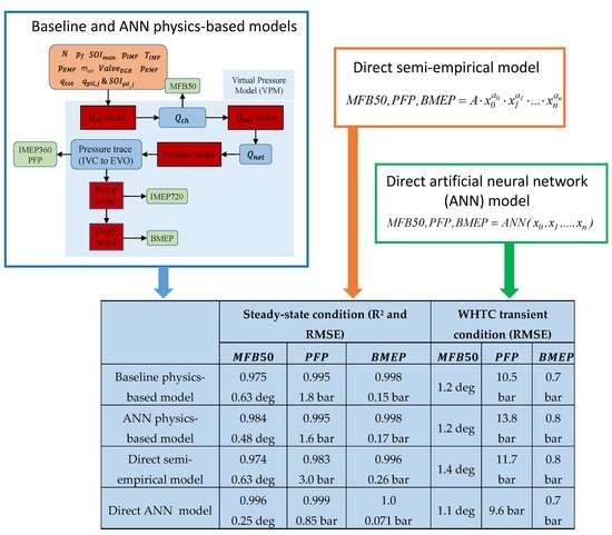
  • Baseline physics-based model: this model was previously presented by the authors in [12] for control-oriented applications. However, in the present study, the model calibration procedure has been refined and the performance of the model has been improved with respect to the previously reported version. In this approach, the tuning parameters are modeled by means of power-law functions, in which the input parameters are the main engine operating variables.
  • ANN physics-based model: this is a new modeling approach, which is based on the use of ANNs to predict the tuning parameters of the aforementioned physics-based model.
  • Direct semi-empirical model: in this approach, semi-empirical correlations, which are constituted by power-law functions, are used to directly estimate MFB50, PFP, and BMEP.
  • Direct ANN model: this approach exploits feed-forward artificial neural networks to directly estimate MFB50, PFP, and BMEP. Details of the methodology used for the training and optimal selection of the number of neurons are also provided in this study.
The four different models have been assessed considering the same experimental dataset, for a 3.0 L FPT diesel engine for light-duty applications, and their performances have been compared under steady-state conditions and in transient operation over a WHTC.
In addition to the comparison of the performance of the previous models, another innovative contribution introduced in this paper concerns the methodology used for the optimal selection of the input parameters of the models. The proposed method is based on the sequential use of the Pearson correlation and partial correlation coefficients, which are used to identify the least and most robust correlation variables that should be excluded or included as model inputs. The use of the Pearson correlation and partial correlation analysis allows the computational effort required for the identification of the input parameters to be reduced significantly.
The paper is organized as follows. Section 2 summarizes the experimental setup and the engine specifications. Section 3 reports the description of the four investigated models. Section 4 is focused on the presentation of the methodology used for the selection of the model input variables. Finally, Section 5 reports the main results, which include:
  • A comparison of the performance of the physics-based model tuned using the methodology introduced in this paper (based on Pearson correlation and partial correlation analysis) with that of the previous version reported in [12].
  • A comparison of the accuracy of the four investigated models under steady-state conditions and in transient operation over a WHTC.
  • A comparison of the performance of the four investigated models, in terms of required computational time, when they are run on an ETAS ES910 (ETAS, Stuttgart, Germany) rapid prototyping device.
This research is a first step towards the development of a model-based combustion controller, which will be developed and tested on the real engine, through rapid prototyping, in the near future.

2. Experimental Setup and Engine Conditions

The experimental tests were run on a Euro VI FPT F1C 3.0 L diesel engine (FPT Motorenforschung AG, Arbon, Switzerland), within a research project conducted in collaboration with FPT Industrial [11]. The activity was carried out in the dynamic test bench facility at the Politecnico di Torino. The main technical specifications of the engine are reported in Table 1.
The fuel is characterized by a density of 835 kg/m3 at 14 °C, a viscosity of 2 mm2/s at 40 °C and a cetane number equal to 43. The considered injection pattern features two pilot shots and a main shot.
The engine is shown in Figure 1. It is equipped with a VGT turbocharger, a short-route cooled EGR system and a flap valve located on the exhaust side downstream from the turbine. Details about the layout of the engine, the test bench and the used sensors (including the main accuracy) have already been described in detail in [38] and are not repeated in this paper for the sake of brevity.
An ETAS ES910 rapid prototyping device, which is equipped with a main Freescale PowerQUICCTM III MPC8548 processor with an 800 MHz clock, was used to verify the computational time required for the models investigated in this paper.
The experimental tests were conducted under steady-state and transient conditions. The steady-state tests have been divided into three categories (Figure 2):
  • a complete engine map (123 tests, indicated with the blue circles in Figure 2).
  • EGR-sweep tests (162 tests, carried out on the points indicated with the red diamonds in Figure 2).
  • sweep tests of the main injection timing (SOImain) and injection pressure (pf) (125 tests, carried out on the points indicated with the black circles in Figure 2).
Validation of the methods was carried out over a WHTC. Details on these validations are given in Section 5.

3. Description of the Models

3.1. Physics-Based Model

Although the physics-based combustion model has already been presented in other studies, a summary of the approach and of the main equations is reported hereafter.
A scheme of the model is shown in Figure 3.
N in Figure 3 indicates the engine speed, while pIMF and TIMF the intake manifold pressure and temperature, respectively, pEMF the exhaust manifold pressure, SOImain the start of injection of the main pulse, SOIpil,j the start of injection of the pilot pulse j, qpil,j the injected fuel quantity of pilot injection j, qtot the total injected fuel quantity, ValveEGR the opening position of the high pressure EGR valve and mair the fresh air trapped mass per cycle/cylinder.
The first step consists in the evaluation of the chemical heat release, according to the following equations (AFM approach):
d Q c h , p i l , j d t ( t ) = K p i l , j _ [ Q f u e l , p i l , j ( t τ p i l , j _ ) Q c h , p i l , j ( t ) ]
d Q c h , m a i n d t ( t ) = K 1 , m a i n _ [ Q f u e l , m a i n ( t τ m a i n _ ) Q c h , m a i n ( t ) ] + K 2 , m a i n _ d Q f u e l , m a i n ( t τ m a i n _ ) d t
Q f u e l , j ( t ) = t S O I , j t m ˙ f , i n j ( t ) H L d t    t t E O I , j
Q f u e l , j ( t ) = t S O I , j t E O I , j m ˙ f , i n j ( t ) H L d t    t > t E O I , j
Q c h = j = 1 n Q c h , j
where j indicates the generic injection pulse, HL indicates the lower heating value of the fuel, and K and τ are the combustion rate coefficient and ignition delay coefficients, respectively.
Subsequently, the net energy of the charge (Qnet) is calculated as follows:
Q n e t , h t Q c h m f , i n j H L Q h t , g l o b _ m f , i n j H L
Q n e t Q n e t , h t Q f , e v a p _
where Qf,evap and Qht,glob indicate the fuel evaporation heat from SOI to SOC and the heat exchanged by the charge with the walls over the combustion cycle; m f , i n j is the total injected fuel mass per cyc/cyl. Qnet is then used to derive the in-cylinder pressure, which is based on the inversion of a single-zone thermodynamic model [39]:
p i = Δ Q n e t p i 1 2 ( V i V i 1 ) + 1 γ 1 p i 1 V i 1 V i V i 1 2 + V i γ 1    ( γ = 1.4 ,    v a l i d f r o m     S O C    t o    E O C )
The compression and expansion phases are modeled with polytropic processes:
p V n _ = c o n s t     ( v a l i d f r o m    I V C    t o    S O C )
p V n _ = c o n s t     ( v a l i d f r o m    E O C    t o    E V O )
while the pressure at IVC (i.e., the starting condition) is correlated with the pressure in the intake manifold:
p I V C = p I M F + Δ p I M F _
The main combustion metrics, that is, MFB50, IMEP360 (gross Indicated Mean Effective Pressure) and PFP (Peak Firing Pressure), can now be evaluated. Finally, friction (FMEP) and pumping (PMEP) models are used, and the net IMEP (IMEP720) and BMEP (Brake Mean Effective Pressure) are estimated:
IMEP 360 = 0 360 p d V V 0
IMEP 720 = IMEP 360 PMEP
BMEP = IMEP 720 FMEP
The tuning parameters of the physics-based model are underlined in Equations (1)–(14).
The Chen-Flynn approach [40] was adopted to estimate FMEP:
FMEP = x 1 + x 2 N + x 3 N 2 + x 4 PFP
where x1–4 are fitting parameters.
The intake oxygen concentration (O2) is an operating variable that is closely correlated with the combustion process, and it is therefore used as an input variable in several sub-models. It is measured, on the experimental test bench, by means of a paramagnetic sensor, which is included in the test cell gas analyzer. However, if the developed combustion model is intended to be used for model-based control, this sensor is not available onboard, and O2 therefore needs to be estimated by means of a specific sub-model.
The following function has been used to estimate O2 [11,41]:
O 2 = x 1 X r , E G R R A F + x 2
where x1–2 are fitting parameters, RAF is the relative air-to-fuel ratio and Xr,EGR is the EGR rate.
Therefore, it is necessary to estimate RAF and Xr,EGR in order to evaluate the intake O2 concentration. The relative air-to-fuel ratio is defined as follows:
R A F = m a i r m f , i n j A F s t
where m a i r is the trapped air mass, mf,inj is the injected fuel mass and AFst is the stoichiometric air-to-fuel ratio (taken as 14.4 in this work).
The accuracy of the estimation of RAF depends to a great extent on the accuracy of the estimation of mair. If mair is obtained from the engine air flow sensor, its accuracy is generally not very high (the error is typically of the order of 5%).
An alternative way of estimating RAF (the method that was adopted in this study) is to develop a semi-empirical correlation, such as:
R A F = x 1 p I M F x 2 T I M F x 3 m f , i n j x 4
where x1–4 are fitted parameters. The correlation is fitted using a calibration dataset, in which the experimental values of RAF are obtained from steady-state measurements carried out using an accurate sensor ( Bosch Lambda sensor LSU 4.9 (Bosch, Gerlingen, Germany)).
With reference to the EGR rate Xr,EGR, it is defined as follows:
X r , E G R = m E G R m E G R + m a i r
where mEGR is the trapped EGR mass.
The EGR rate can in general be derived experimentally on the basis of the measured emissions and of the measured intake CO2 concentration. However, if the combustion model is intended to be applied for control-oriented applications, a real-time estimation of the EGR rate is needed, through the use of a dedicated submodel. To this aim, several approaches can be used (e.g., see [41]).
The simplest method to estimate the EGR rate (which was adopted in this paper) is to resort to look-up tables that depend on the engine speed and pedal position. These look-up tables were derived on the basis of the analysis of steady-state measurements.
As far as the calibration procedure is concerned, as reported in the previous sections, the physics-based model is characterized by several tuning parameters, which are mentioned in Table 2.
The calibration of these parameters is carried out in two steps.
In the first step, the optimal values of all the parameters are identified, test by test, on the basis of the available experimental data. The process used for the identification of these values is reported in detail in [16], and is based on the best matching between the experimental and predicted heat release and in-cylinder pressure curves. At the end of this first step, a dataset of the optimal values of the model calibration parameters is available.
In the second step, on the basis of the dataset identified in step 1, the model calibration parameters are correlated with input variables, which are generally related to the engine operating conditions (e.g., intake manifold pressure/temperature, intake oxygen concentration, engine speed and load…), using such mathematical methods as look-up tables, empirical or semi-empirical functions or machine learning tools. Semi-empirical correlations, based on power-law functions, are used in the baseline version of the physics-based model (see [12]), since they are capable of capturing the non-linear behavior of the correlations. However, in previous studies, the input parameters for these correlations were identified on the basis of a trial and error approach.
In the next sections, two aspects are investigated in order to improve the physics-based model with respect to previously reported versions:
  • A new procedure for the identification of the optimal set of input parameters is developed. This procedure is based on the joint use of the Pearson correlation analysis, partial correlation analysis, and sensitivity analysis, and it allows the performance of the baseline physics-based model to be improved with respect to the previously developed versions.
  • An alternative mathematical method (i.e., ANNs) is used to estimate the model calibration parameters:
    K p i l , K 1 , m a i n , = ANN ( x 0 , x 1 , , x n )
    where x0, x1,…, xn are correlation variables. This approach has never been investigated before, and is denoted as “ANN physics-based model”.

3.2. Direct Semi-Empirical Models

In addition to the baseline and ANN physics-based models, semi-empirical correlations were also developed in order to directly predict the MFB50, PFP, and BMEP metrics.
These correlations are based on power-law functions of the type:
MFB 50 , PFP , BMEP = A x 0 a 0 x 1 a 1 x n a n
The identification of the x0, x1xn correlation variables and the fitting of the model are analyzed in the next sections. The semi-empirical models are trained on the basis of the same experimental data used for the physics-based model calibration.

3.3. Direct Artificial Neural Networks

The final method investigated to predict MFB50, PFP, and BMEP is based on feed-forward artificial neural networks with one inner layer:
MFB 50 , PFP , BMEP = ANN ( x 0 , x 1 , , x n )
where x0, x1,…, xn are the input variables of the neural networks.
The networks are trained on the basis of the same experimental data used for the physics-based model calibration. The methodology used for the calibration of the model, including the selection of the optimal number of neurons, is discussed in detail in Section 5.

4. Selection of the Model Input Variables

Selecting the most appropriate input parameters as independent variables for all the previously mentioned approaches is a key-aspect to obtain accurate and robust models.
In this paper, optimal sets of input parameters have to be defined for:
  • The power-law correlations or the ANNs that evaluate the calibration parameters of the baseline physics-based model and of the ANN physics-based model, respectively.
  • The direct semi-empirical model that estimates MFB50, PFP, BMEP.
  • The direct ANN model that estimates MFB50, PFP, BMEP.
In general, the input parameters are related to the engine operating conditions, and can be either directly measured quantities or derived quantities. The directly measured parameters (such as engine speed N, the start of injection of the pilot/main pulses SOIpil/SOImain, the total injection quantity of the pilot pulses qpil,tot, the injection quantity of the main pulse qmain, the total injection quantity qtot, the intake/exhaust pressure and temperature pIMF,TIMF/pEMF,TEMF, the common rail pressure pf, the trapped air mass mair and the EGR valve opening position ValveEGR) are the most commonly used input variables for control-oriented applications, since they are readily available for the ECU without the need of any additional sub-model. However, derived parameters (such as intake density ρIMF, in-cylinder gas density and temperature at the start of each injection pulse ρSOI,pil, ρSOI,main, TSOI,pil, TSOI,main, the start of combustion of the pilot and main pulses SOCpil/SOCmain, in-cylinder gas density and temperature at the start of combustion for each injection pulse ρSOC,pil, ρSOC,main, TSOC,pil, TSOC,main, the pressure difference between the exhaust and intake manifold Δpexh-int) or even outcomes of sub-models (such as PFP, MFB50) have also been used as input variables in models reported in the literature, since their correlation with the dependent variables is sometimes greater than that of the directly measured parameters. In this study, all these kinds of parameters were initially considered as candidate input variables to develop the models.
Table 3 reports the list of the directly measured input parameters (1st column), of the generated parameters (from the directly measured ones or from the combustion model) which can be used as input parameters (2nd column), and of the dependent output variables which have been considered in the present investigation. A total of 46 parameters have been included. It should be noted that some of the dependent variables are the calibration parameters of the physics-based model, which needs to be estimated for the model application (3rd column), while MFB50, PFP, and BMEP are the combustion metrics that are adopted for combustion control applications, i.e., the final output variables of all the four modeling approaches that have been investigated in this study (4th column).
The procedure that was identified to select the optimal set of input parameters is based on the joint use of the Pearson correlation and partial correlation coefficients (see [42,43,44,45] for details concerning the use of these coefficients), and is reported in detail in Appendix A for the paper readability purposes. However, a synthetic description is reported hereafter.
Basically, the procedure involves 3 steps:
  • First, the Pearson correlation coefficient is calculated for all the possible combinations of the 46 variables reported in Table 3 (the results are reported in Appendix A in Table A1). This coefficient measures the linear dependence between two variables, xi and xj, and is defined as follows:
    ρ ( x i , x j ) = cov ( x i , x j ) var ( x i ) var ( x j )
    where cov(xi, xj) is the covariance between xi and xj, while var(xi) and var(xj) are the variances of xi and xj, respectively. The Pearson correlation coefficient varies between −1 and +1.
    After the analysis of the Pearson correlation coefficients, an initial candidate set of input variables is identified for each output quantity that has to be estimated (see Table A2 in Appendix A).
  • In the second step, the partial correlation coefficient is evaluated between the dependent variables and each input variable of the initial candidate set, when removing the effect of the remaining input variables of the same set. It should be recalled that the partial correlation coefficient is able to measure the linear dependence between two variables, xi and xj, when the effect of the other input variables variable (z1, z2,…, zi) is removed:
    ρ ( x i , x j ; z 1 , z 2 , , z i ) = ρ ( x i , x j ; z 1 , z 2 , , z i 1 ) ρ ( x j , z i ; z 1 , z 2 , , z i 1 ) ρ ( x i , z i ; z 1 , z 2 , , z i 1 ) [ 1 ρ ( x j , z i ; z 1 , z 2 , , z i 1 ) 2 ] [ 1 ρ ( x i , z i ; z 1 , z 2 , , z i 1 ) 2 ]
    The partial correlation coefficient is more robust than the Pearson coefficient. However, the number of parameters should not be too high, otherwise, the consistency of the method decreases. Also, the partial correlation coefficient varies between −1 and +1. As reported in Appendix A (see Table A3), the simultaneous analysis of the Pearson and of the partial correlation coefficients has allowed the least and most robust correlation variables of the initial candidate set to be identified for each dependent output variable. Therefore, some variables were excluded from the initial candidate set identified in step 1 (since they showed low values of the Pearson and partial correlation coefficients), while other variables were kept since they showed high values of both the Pearson and partial correlation coefficients.
  • The remaining correlation variables of the initial candidate set which showed intermediate values of the Pearson and partial correlation coefficients were analyzed on the basis of a sensitivity analysis, in order to identify those that had to be kept and those that had to be excluded. A power law function, such as that reported in Equation (21), was used to model each output dependent parameter, and all the possible combinations of input variables were identified by evaluating, for each combination, the related model fitting precision, which was quantified by a correlation coefficient Radj:
    R a d j = 1 n exp 1 n exp k ( 1 R 2 )
    where nexp is the total number of experimental data and k is the total number of free coefficients. The adjusted correlation coefficient Radj takes into account the number of available experimental tests used for the model fitting, in relation to the number of free parameters of the model. In the end, the combinations which led to the best trade-off between the prediction accuracy and the number of input parameters were selected. Details on the sensitivity analysis have not been reported in this paper for the sake of brevity.
It should be noted that the proposed approach, i.e., the preliminary selection of the input variables through Pearson and partial correlation coefficients, and the subsequent sensitivity analysis carried out on a reduced set of variables, is more computationally efficient than a pure sensitivity analysis approach which includes the entire set of input variables.
In fact, the number of possible combinations that have to be investigated in the sensitivity analysis can be calculated through the following formula:
N c = 2 j 1
where Nc is the number of possible combinations for the sensitivity analysis and j is the number of independent variables.
According to Equation (26), Nc increases to a great extent as j increases. Therefore, the combined use of the Pearson correlation and partial correlation analysis is a very useful and efficient way of decreasing the computational effort of the sensitivity analysis, since it allows the poorly correlated variables to be excluded a-priori, or the highly correlated variables to be selected, so that the sensitivity analysis (which is highly time consuming, since it requires model fitting of each possible combination), is only carried out for a reduced set of variables.

5. Results and Discussion

The improvement in the prediction performance of the physics-based model (compared to the previous version reported in [12]), when adopting the new methodology for the input parameter selection described in Section 4, is reported first. Subsequently, the performances of the four investigated models described in Section 3 are compared, in terms of accuracy at steady-state conditions and over WHTC, and in terms of required computational time. The main advantages and drawbacks of each kind of approach are also discussed.

5.1. Improvement to the Baseline Physics-Based Combustion Model

The performance of the baseline physics-based combustion model has been improved, with respect to the previous version reported in other papers [12]. The set of input variables for the model correlations has been revised, on the basis of the Pearson correlation and partial correlation analysis, according to the procedure described in the previous section.
The final list of selected input variables for each dependent variable and the corresponding fitting precision are shown in Table 4. It should be noted that some correlations are improved with respect to pure power-law functions.
Figure 4 and Figure 5 report the accuracy of the original physics-based model with the baseline calibration (presented in [12]) and the revised model which embeds the improved correlations, concerning the estimation of BMEP, PFP, and MFB50, for the steady-state tests reported in Figure 2.
It can be seen that, although the accuracy in the estimation of BMEP is somewhat similar, an improvement in the estimation of PFP, and MFB50 can be obtained, since the related RMSE values decrease from 2.47 bar to 1.82 bar and from 0.86 deg to 0.63 deg, respectively.

5.2. Direct Semi-Empirical Models of MFB50, PFP, and BMEP

The procedure used to identify the input parameters of the physics-based model, which was described in Section 4, was also adopted to select the input variables of the direct semi-empirical models. The correlations identified for MFB50, PFP, and BMEP are reported in Table 5.

5.3. ANN-Based Models

Artificial neural networks have a great capacity to capture complex nonlinear relationships between variables through relatively simple mathematical operations, and require very little computational effort. Therefore, they are good candidates for control-oriented applications. In this section, ANNs have been used to:
  • Replace the power law-based correlations of the physics-based models shown in Table 4. The resulting new physics-based model is referred to as “ANN physics-based model”.
  • Directly simulate the MFB50, PFP, and BMEP combustion metrics, analogously to the semi-empirical models shown in Table 5.
In both cases, the sets of input variables that were used for the ANNs are the same as those shown in Table 4 (physics-based model) and Table 5 (semi-empirical models). The experimental data used for ANN training is constituted by the 410 tests shown in Figure 2.
In general, the implementation of ANNs involves three steps: the selection of the input variables, the training phase, and the testing phase. The available experimental dataset is usually split randomly for training, testing and validation purposes. The main parameters that have to be selected are the net type, the number of inner layers and the number of neurons for each layer, the activation function, and the training algorithm.
As far as the network type is concerned, feed-forward networks are typically used in the literature, and have also been used in this paper. These types of networks contain an input layer, some hidden layers, and an output layer. The back-propagation training algorithm is generally used as a training algorithm for feed-forward neural networks [46]. The Bayesian regularization training function ‘trainbr’ is one of the best-known BP training algorithms; it can lead to very precise ANNs [46,47] and is able to provide good generalization for difficult, small or noisy datasets [48], even though its number of epochs is usually higher. In this work, the training dataset is not large and the network structure is quite simple, therefore a relatively large epoch number should not lead to an unacceptably long computation time. For these reasons, ‘trainbr’ was selected as the training algorithm.
In order to speed up the learning process for a high number of networks, the inputs are usually normalized before sending them to the input layer. In this work, the ‘mapminmax’ process function [49] has been used to normalize the inputs, so that all the values fall into the [−1, 1] interval. Similarly, network outputs can also be associated with processing functions [49].
The activation function that was used in this work is the ‘tansig’ function. It was found, with reference to the number of hidden layers, that one layer was enough to simulate the parameters of the physics-based model and the combustion metrics (MFB50, PFP, BMEP). The use of one hidden layer for feed-forward neural networks is also quite common in the literature [47,50,51], especially when the number of training data is not very high.
The MSE minimization criterion was used for the training process, as suggested in [52]. The ANN performance is evaluated by comparing the network outputs with the experimental data through regression analysis [53]. The values of the mean-squared-error MSE and the determination coefficient R2 are used to measure the performance of ANNs. Details of the ANN parameters developed on the MATLAB (R2016b, MathWorks, Natick, MA, USA) platform are shown in Table 6.
The optimal number of neurons in the hidden layer depends on the specific application, and it cannot, therefore, be identified a-priori. The ANN predictive performance is influenced to a great extent by the number of neurons. According to the literature, a too large number of neurons may lead to overfitting, while a too small number of neurons may make the ANN too simple to be able to capture the characteristics of a complex system (that is, underfitting [37]). Therefore, a trade-off must be made between the number of hidden layer neurons and the predictive performance of the ANN, and a sensitivity analysis is always needed in order to identify what the optimal number of neurons is for a specific application. In this section, a suitable number of neurons is selected for each of the dependent parameters that have to be estimated (i.e., those reported in Table 4 and Table 5).
All the available steady-state experimental data (410 tests) were used to generate the ANNs. Overall, 80% of the data was used as training data, and the other 20% was used to test the trained ANNs. Considering the smallness of the training dataset, the training process features some uncertainties, because the initial value of the weights of the neural networks is generated randomly. Thus, when the training process of a given neural network is repeated, its performance may vary to a great extent, even when the same input training dataset is used. Moreover, the experimental dataset for each training process is randomly divided into training and testing datasets with a certain ratio. This can also influence the performance of the trained neural networks when the training process is repeated. However, it has been shown in the literature that these uncertainties decrease considerably, and may even be ignored, when the size of the training dataset is sufficiently large [54], but this was not the case in this study.
Therefore, 200 training and testing repetitions were carried out for each ANN, with random initial weights and random splitting of the experimental dataset into training and testing datasets. The determination coefficient R2 and the mean square error MSE were used to measure the performance of the ANNs. The mean values of R2 and MSE for 200 trials were calculated for the training and testing of each ANN.
The trade-off between the number of hidden layer neurons and the performance of the ANN was explored for each ANN that simulated the parameters of the physics-based model (in the “ANN physics-based model”) and for each ANN that simulated the MFB50, PFP, and BMEP combustion metrics (in the “direct ANN model”). The results of the sensitivity analysis are shown in Appendix B.
The sensitivity analysis allowed the optimal number of hidden layer neurons to be identified for each parameter. The most suitable number of neurons for each parameter is listed in Table 7, along with the mean values of R2 and MSE for the training and testing phases. In general, it can be seen that the most suitable neuron number is no higher than 7 in all cases.
Once the sensitivity analysis had been carried out, the best ANN out of the 200 training trials was selected on the basis of the criteria reported in Appendix B for each parameter.
After this stage, the following investigations were conducted
  • With reference to the physics-based model, the power law-based correlations of the calibration parameters were replaced by the corresponding ANNs, and the performance of the resulting model (i.e., the “ANN physics-based model”) was evaluated. Table 8 shows a comparison between the accuracy of the ANN-based correlations and of the power-law based ones in the estimation of the parameters of the physics-based model. It can be observed that all the precisions based on ANNs are higher than those based on the power law correlations. ANNs have in fact been proved to have a powerful ability to catch the non-linear characteristics between input and output parameters
  • The performance of the ANNs that were used to directly simulate MFB50, PFP, and BMEP was evaluated
A detailed comparison of the performance of the four developed approaches, for the estimation of the MFB50, PFP, and BMEP combustion metrics, is reported in the next section.

5.4. Comparison of the Four Different Models under Steady-State and Transient Conditions

In this section, the performance of the four different models has been tested under steady-state and transient operating conditions.
First, the performance of the developed models was compared under steady-state conditions.
The results are shown in Figure 6.
It can be seen, from the previous charts, that the accuracy of the ANN physics-based model is higher than that of the baseline physics-based model concerning MFB50 and PFP. This indicates that the ANNs are more powerful than the power-function-based empirical functions in catching the nonlinear characteristics between the input and dependent parameters of the model for these two metrics under steady-state conditions. Overall, the accuracy of the direct ANN model is the best, while the accuracy of the semi-empirical model is the lowest. However, the absolute values of the error of the semi-empirical model are still acceptable, considering that this kind of model ignores the detailed simulation of the in-cylinder physical process and requires a limited number of free parameters to be tuned (as a consequence, it also requires a limited number of experimental calibration tests). This suggests that the semi-empirical model, based on power functions, is also suitable for control-oriented combustion control applications, since its computational effort is much less than that of the physics-based model.
The performance of the developed models was then evaluated and compared under transient operating conditions over WHTC. The results are shown in Figure 7, Figure 8 and Figure 9.
Table 9 reports a summary of the accuracy of the models over WHTC and under steady-state operating conditions.
It can be seen from the graphs of Figure 6, Figure 7, Figure 8 and Figure 9 and from Table 9 that the accuracy of the direct ANN model is the best among all the different approaches, not only for steady-state operation (RMSE equal to 0.25 deg, 0.85 bar and 0.071 bar for MFB50, PFP, and BMEP, respectively), but also for transient operation over WHTC (RMSE of 1.1 deg, 9.6 bar and 0.7 bar for MFB50, PFP, and BMEP, respectively).
The accuracy of the baseline physics-based model under transient operating conditions is slightly lower than that of the direct ANN model in terms of RMSE (1.2 deg vs. 1.1 deg for MFB50, 10.5 bar vs. 9.6 bar for PFP, 0.7 bar vs. 0.7 bar for BMEP), but is higher than that of the ANN physics-based model (1.2 deg vs. 1.2 deg for MFB50, 10.5 bar vs. 13.8 bar for PFP, 0.7 bar vs. 0.8 bar for BMEP) and of the semi-empirical model (1.2 deg vs. 1.4 deg for MFB50, 10.5 bar vs. 11.7 bar for PFP, 0.7 bar vs. 0.8 bar for BMEP).
A remarkable result is the deterioration of the accuracy of the ANN physics-based model (compared to the baseline physics-based model) which occurs for transient operation, while this approach leads to more accurate results for steady-state conditions. Therefore, this approach lacks robustness, compared to the baseline physics-based model.
Finally, the semi-empirical model shows a lower level of accuracy than the baseline physics-based model and the direct ANN model. However, the accuracy deterioration can still be considered acceptable, considering the simple structure of this model and the low calibration effort that is required, as discussed above.
Overall, the direct ANN model can be considered as the best candidate for control-oriented applications, since:
  • it is much simpler in structure and theory and easier to build than the physics-based model;
  • it does not require any detailed knowledge or modeling of the physical and chemical processes;
  • it is robust not only under steady-state conditions, but also for transient operation;
  • its accuracy is high even when a not so large dataset of experimental tests (410) is used for training;
  • it features the best accuracy under steady-state and transient operating conditions;
  • the required computational time is less than that of the physics-based model (see the next section).
The main drawback of ANNs is that they are a black-box type models, so they do not provide detailed information about the physical and chemical processes which occur inside the combustion chamber (e.g., heat release trend, in-cylinder pressure, temperatures …).

5.5. Analysis of the Computational Time

The computational time of all the models (excluding the ANN physics-based model, which was found to be the least robust approach) was estimated when they were run on the ETAS ES910 device. The results are reported in Table 10.
It can be seen that the direct ANN direct model and the semi-empirical model feature the lowest computational times, so that they can be considered the most suitable approaches to be implemented on an ECU for onboard control. The physics-based model requires the highest computational time. However, it is also compatible with real-time combustion control applications, since it is much lower than the typical engine cycle time. On the basis of the results reported in this study, a model-based combustion controller will be developed in the near future, and will be tested on the engine through the ETAS ES910 rapid prototyping device.

6. Conclusions

A comparison of the performance of physics-based, semi-empirical and artificial neural network (ANN)-based models has been carried out in this paper to estimate the main combustion metrics for an FPT Euro VI 3.0 L F1C diesel engine. The models were developed for combustion control-oriented applications. The combustion metrics that are predicted by the models are MFB50, PFP, and BMEP. These metrics are interesting for control-oriented applications, since they are closely related to the thermal efficiency and to the pollutant formation process of the engine. Four different types of modeling approaches have been investigated. The first approach is based on a previously developed low-throughput mean-value physics-based model, which is capable of simulating the heat release rate, the in-cylinder pressure, and the related metrics on the basis of the accumulated fuel mass principle. In this approach, the tuning parameters of the model are estimated on the basis of physically-consistent correlations, which are modeled using power-law functions. The second investigated approach is based on the joint use of artificial neural networks (ANNs) and physical modeling: instead of using the power-law functions, ANNs have been used to identify the parameters of the physics-based model. The third investigated approach is based on a direct estimation of MFB50, PFP, and BMEP on the basis of semi-empirical correlations. The fourth approach is based on the use of ANNs to directly estimate MFB50, PFP, and BMEP. The performance of the four models was evaluated under steady-state conditions and transient operation over WHTC.
Moreover, a new methodology, which is based on the sequential use of the Pearson correlation and partial correlation analysis, has been developed to identify the optimal set of input model parameters in order to a priori identify the correlation variables that should be excluded and the most robust correlation variables.
The main results can be summarized as follows:
(1)
The new methodology set up for the identification of the model input parameters has allowed an improvement to be obtained in the calibration of the baseline physics-based model. Although the accuracy in the estimation of BMEP is quite similar, an improvement in the estimation of PFP, and MFB50 can be obtained, since the related RMSE values decrease from 2.47 bar to 1.82 bar and from 0.86 deg to 0.63 deg, respectively, at steady-state conditions. Moreover, it allows a saving in the model calibration computational time to be achieved.
(2)
The direct ANN model has shown the best accuracy in the estimation of MFB50, PFP, and BMEP under both steady-state conditions (RMSE = 0.25 deg, 0.85 bar and 0.071 bar, respectively) and transient operation over the WHTC (RMSE = 1.1 deg, 9.6 bar and 0.7 bar, respectively); the accuracy of the baseline physics-based model is slightly worse than that of the direct ANN model (RMSE = 0.63 deg, 1.8 bar, 0.15 bar under steady-state conditions, RMSE = 1.2 deg, 10.5 bar, 0.8 bar over WHTC).
(3)
The accuracy of the ANN physics-based model is higher than that of the baseline physics-based model under steady-state operations (RMSE = 0.48 deg, 1.6 bar, 0.17 bar), but it shows a marked deterioration for transient operation (RMSE = 1.2 deg, 13.8 bar, 0.8 bar), and this approach, therefore, seems to lack robustness.
(4)
The accuracy of the semi-empirical model is worse than that of the physics-based model and of the direct ANN model under steady-state conditions (RMSE = 0.63 deg, 3 bar, 0.26 bar) and over the WHTC (RMSE = 1.4 deg, 11.7 bar, 0.8 bar). However, the accuracy can still be considered acceptable, in view of the simple mathematical structure of this kind of model, and the low number of tuning parameters that are necessary (and therefore of experimental data needed for calibration).
(5)
The computational time required for the direct ANN model and semi-empirical model is less than 50 μs on an ETAS ES910 rapid prototyping device, while that of the baseline physics-based model is of the order of 350 μs.
Overall, the direct ANN model can be considered the best candidate for control-oriented applications, since:
  • it is much simpler in structure and theory and easier to build than the physics-based model;
  • it does not require any detailed knowledge or modeling of the physical and chemical processes;
  • it is robust not only under steady-state conditions, but also in transient operation;
  • its accuracy is high, even when a not so large dataset of experimental tests (410) is used for training;
  • it features the best accuracy under steady-state and transient operating conditions
  • the required computational time is lower than that of the physics-based model.
The main drawback of this kind of model is that it is of the black-box type. Thus, it does not provide detailed information about the physical and chemical processes that occur inside the combustion chamber, such as the heat release trend, in-cylinder pressure, or temperatures.

Author Contributions

The authors contributed equally to the preparation of the paper. Conceptualization, S.H., R.F., S.d.; Methodology, S.H., R.F., S.d.; Software, S.H.; Formal Analysis, S.H., R.F., S.d.; Data Curation, A.M. (Andrea Manelli), L.V., S.d.; Writing-Original Draft, S.H., R.F.; Writing-Review and Editing, R.F., M.M., A.M. (Antonio Mittica); Supervision, R.F., S.d., A.M. (Antonio Mittica), H.W., Y.W.

Funding

FPT is kindly acknowledged for its support in the activities. This work was also supported by the China Scholarship Council (Grant No. 201706680011) and Marine Low-Speed Engine Project-Phase I (CDG01-KT0302). The authors would like to thank Omar Marello for his efforts in discussing and carrying out this research.

Conflicts of Interest

The authors declare no conflict of interest.

Abbreviations

ABDCAfter Bottom Dead Center
AFststoichiometric air-to-fuel ratio
ANNartificial neural network
BMEPBrake Mean Effective Pressure (bar)
CFDComputer Fluid-Dynamics
DoEDesign of Experiment
ECUEngine Control Unit
EGRExhaust Gas Recirculation
EOCEnd of Combustion
EOIEnd of Injection
EVOExhaust Valve Opening
FMEPFriction Mean Effective Pressure (bar)
HLlower heating value of the fuel
HCCIHomogeneous Charge Compression Ignition
ICEInternal Combustion Engines
IMEP360gross Indicated Mean Effective Pressure (bar)
IMEP720net Indicated Mean Effective Pressure (bar)
IVCIntake Valve Closing
Kcombustion rate coefficient
mmass
mairtrapped air mass
mEGRtrapped EGR mass
mf,injinjected fuel mass (mg per cycle/cylinder)
m ˙ f , i n j fuel injection rate
MFB50crank angle at which 50% of the fuel mass fraction has burned (deg)
npolytropic coefficient for the compression phase
n’polytropic coefficient for the expansion phase
Nengine rotational speed (1/min)
O2intake charge oxygen concentration (%)
ppressure (bar)
PCCIPremixed Charge Compression Ignition
pEMFexhaust manifold pressure (bar abs)
pfinjection pressure (bar)
PFPpeak firing pressure
pIMFintake manifold pressure (bar abs)
PMEPPumping Mean Effective Pressure (bar)
qinjected fuel volume quantity (mm3)
Qchchemical heat release
Qf,evapfuel evaporation heat
qmaintotal injected fuel volume quantity of the main pulse per cycle/cylinder
qtottotal injected fuel volume quantity per cycle/cylinder
qtot,piltotal injected fuel volume quantity of the pilot pulses per cycle/cylinder
Qfuelchemical energy associated with the injected fuel
Qht,globglobal heat transfer of the charge with the walls
Qnetnet heat release
R2squared correlation coefficient
RAFrelative air-to-fuel ratio
RMSroot mean square
RMSEroot mean square error
SOCstart of combustion
SOIelectric start of injection
SVPsupport vector machine
ttime
Ttemperature (K)
TEMFexhaust manifold temperature
TIMFintake manifold temperature
TSOCcharge temperature at start of combustion
TSOIcharge temperature at start of injection
Vvolume
V2XVehicle-to-Everything
ValveEGRopening position of the high pressure EGR valve
VGTVariable Geometry Turbine
WHTCWorldwide Harmonized Heavy-duty Transient Cycle
Xr,EGREGR rate

Greek Symbols

Δpexh-intdifference between the exhaust and intake manifold pressure
γisentropic coefficient
ρdensity
ρIMFdensity in the inlet manifold
ρSOCcharge density at the start of combustion
ρSOIcharge density at the start of injection
τignition delay coefficient

Appendix A. Correlation Analysis for the Selection of the Model Input Variables

In order to make the correlation analysis more synthetic, the considered variables have been associated with indexing numbers (IN), as shown in Table A1.
Table A1. Collected variables and corresponding index number (IN).
Variable NameINVariable NameINVariable NameINVariable NameIN
N 1 V a l v e E G R 13 T S O C , m a i n 25 Q n e t m a x 37
p f 2 X r E G R 14 S O C p i l 26 Δ p I M F 38
S O I p i l 3 R A F 15 S O C m a i n 27 n 39
S O I m a i n 4 O 2 16 Δ p e x h i n t 28 n 40
q t o t , p i l 5ρIMF17 τ p i l 29PFP41
q m a i n 6 ρ S O I , p i l 18 τ m a i n 30IMEP36042
q t o t 7 ρ S O I , m a i n 19 K p i l 31PMEP43
p I M F 8 ρ S O C , p i l 20 K 1 , m a i n 32FMEP44
T I M F 9 ρ S O C , m a i n 21 K 2 , m a i n 33IMEP72045
pEMF10 T S O I , p i l 22MFB5034BMEP46
TEMF11 T S O I , m a i n 23 Q h t , g l o b 35
m a i r 12 T S O C , p i l 24 Q f , e v a p 36
For the sake of clarity, Figure A1 reports the temporal sequence of the calculation of the different variables used in the physics-based model.
Figure A1. Temporal calculation sequence of the physics-based model variables.
Energies 12 03423 g0a1
The Pearson correlation coefficient was calculated, using Matlab R2016b, in order to identify the correlations between the variables identified in Table A1. The results are reported in Figure A2.
The numbers in the rows and columns in Figure A2 are the indexing numbers of the variables shown in Table A1. The background color changes from green to white and from white to red when the Pearson coefficient value varies in the (−1, 0) range or in the (0, 1) range, respectively. The linear relationship between two variables is considered strong when their Pearson coefficient value is in the (−1.0, −0.5) or (0.5, 1) ranges, moderate when it is in the (−0.5, −0.3) or (0.3, 0.5) ranges, weak when it is in the (−0.3, −0.1) or (0.1, 0.3) ranges, and non-existent or very weak when from it is in the (−0.1, 0.1) range [43].
The Pearson coefficient can provide useful information for the selection of:
  • the input parameters of the correlations which are used to estimate the calibration parameters of the physics-based models (i.e., those reported in Table 3), or the input parameters of the ANNs that are used to estimate the same calibration parameters;
  • the input parameters of the semi-empirical correlations that are used to directly estimate MFB50, PFP, BMEP;
  • the input parameters of the ANNs that are used to directly estimate MFB50, PFP, BMEP.
Figure A2. Pearson correlation coefficients for all the possible combinations of the variables reported in Table A1.
Energies 12 03423 g0a2
As can be seen in Figure A2, the groups of variables [IN 3, IN 4], [IN 6, IN 7], [IN 13, IN 14], [IN 17, IN 19], [IN 20, IN 21], [IN 24, IN 25] and [IN 26, IN 27], namely [SOIpil, SOImain] [qmain, qtot], [ValveEGR, Xr,EGR], [ρIMF, ρSOImain], [ρSOC,pil, ρSOC,main], [TSOC,pil, TSOC,main] and [SOCpil, SOCmain], are very closely correlated to each other, since their crossed Pearson coefficient is almost equal to 1. Therefore, during the identification of the input variables of the models, it is sufficient to select only one of them as representative of each variable group. Moreover, it should be noted that the variables which are calculated at an earlier stage are expected to be closely correlated to the variables that are calculated in a subsequent stage (see Figure A1).
The following rules were identified to select the set of input variables to use in the correlations of the physics-based model or in the semi-empirical and ANN-based models, on the basis of the information derived from the Pearson correlation analysis:
  • the temporal sequences of the variables in the model have to be taken into account, i.e., variables cannot be used as the independent variables if they are calculated or occur after the dependent variable, according to the scheme in Figure A1;
  • the directly measured engine operation variables (namely N, pf, SOI, fuel injection quantity, pIMF, TIMF, ValveEGR) should be considered as independent variable candidates with top priority, because they are the primary cause of the changes in engine operation. Moreover, these variables are usually very precise because they are measured directly in real-time. The generated parameters SOI, TSOI), based on SOI, should be considered with higher priority than those based on SOC SOC, TSOC), because of the uncertainty chain for the estimation of SOC on the basis of SOI;
  • the dependent variables (such as τpil, τmain, SOC, Kpil, K1,main, K2,main, Qf,evap, Qht,glob, n, n’, ΔpIMF, PMEP, FMEP) should be considered with a lower priority as correlation parameters, because they are usually less precise than the directly measured parameters. The Xr,EGR, RAF, O2, ρSOC and TSOC generated parameters should also be considered with a lower priority because of their relatively low precision;
  • some variable groups (e.g., [SOIpil, SOImain] [qmain, qtot], [ValveEGR, Xr,EGR], [pIMF, mair, ρIMF], [ρSOC,pil, ρSOC,main], [TSOC,pil, TSOC,main] and [SOCpil, SOCmain]) are constituted by two variables which are closely correlated to each other. Therefore, only one variable should be selected as representative of each group;
  • the total number of independent variable candidates should not be too high (in this study a maximum of 15 variables was chosen for the estimation of each dependent one), in order to ensure that the partial coefficient order is not too large and to make the model more robust to input uncertainty.
Some considerations should also been made concerning the mair and pEMF variables. Although mair is measured directly, it is usually not a precise or stable variable, since the accuracy of the engine air mass flow sensor is not very high (~5%), and its use, therefore, needs to be evaluated carefully. Moreover, many medium and heavy-duty engines are not generally equipped with air mass flow sensors and the exhaust manifold pressure is generally not measured in production engines, so its use as an input variable for the model should also be evaluated carefully (in this study it was avoided).
On the basis of the rules explained above, an analysis of the Pearson correlation coefficients was carried out to select independent variable candidates for each dependent variable. A summary is reported in Table A2.
It should be recalled that some of the dependent variables are the calibration parameters of the physics-based model (see Table 3), and they need to be modeled through correlations or ANNs, while other dependent variables (i.e., MFB50, PFP, BMEP) are the direct outcome of the semi-empirical model or of the direct ANN model, i.e., the metrics to be used for combustion control applications.
Table A2. Initial candidate set of the input variables for each output parameter, identified on the basis of the Pearson correlation analysis.
Dependent VariableInitial Candidate Set of the Independent Variables Selected Using Pearson Correlation Analysis
R A F N , p f , S O I p i l , q t o t , p i l , q t o t , p I M F , T I M F , X r E G R , ρ S O I , p i l , ρ S O I , m a i n
τ p i l N , p f , S O I p i l , q t o t , p i l , p I M F , T I M F , V a l v e E G R , R A F , ρ S O I , p i l , T S O I , p i l
τ m a i n N , p f , S O I p i l , q t o t , p i l , q t o t , T I M F , m a i r , X r E G R , R A F , ρ S O I , p i l , ρ S O I , m a i n , ρ S O C , p i l , T S O I , p i l , Δ p e x h i n t , τ p i l
K p i l N , p f , S O I p i l , q t o t , p i l , p I M F , T I M F , V a l v e E G R , ρ S O I , p i l , T S O I , p i l , τ p i l , Δ p e x h i n t
K 1 , m a i n N , p f , S O I m a i n , q t o t , p i l , q t o t , p I M F , T I M F , V a l v e E G R , R A F , ρ S O I , m a i n , ρ S O C , p i l
K 2 , m a i n N , p f , S O I p i l , q t o t , p i l , q t o t , T I M F , m a i r , X r E G R , R A F , ρ S O I , p i l , ρ S O I , m a i n , T S O I , m a i n , K 1 , m a i n
Q h t , g l o b N , p f , S O I p i l , q t o t , p i l , q t o t , T I M F , m a i r , X r E G R , R A F , ρ S O I , p i l , ρ S O C , p i l , τ m a i n , K 2 , m a i n
Q f , e v a p N , p f , S O I p i l , q t o t , p i l , q t o t , T I M F , m a i r , ρ S O I , p i l , ρ S O I , m a i n , R A F , V a l v e E G R , T S O I , p i l , Δ p e x h i n t
Δ p I M F N , p f , S O I p i l , q t o t , p i l , q m a i n , p I M F , X r E G R , ρ S O I , p i l , ρ S O I , m a i n , T S O I , p i l , ρ S O C , m a i n , Δ p e x h i n t
n N , p f , S O I p i l , q t o t , p i l , q t o t , p I M F , T I M F , V a l v e E G R , ρ S O I , p i l , ρ S O I , m a i n , T S O I , p i l , T S O I , m a i n , T S O C , m a i n , Δ p e x h i n t
n N , p f , q t o t , p i l , q m a i n , S O I p i l , T I M F , V a l v e E G R , R A F , ρ I M F , ρ S O I , m a i n , T S O I , p i l , Δ p e x h i n t , K 1 , m a i n , K 2 , m a i n
M F B 50 N , p f , S O I m a i n , q t o t , p i l , q m a i n , T I M F , X r E G R , R A F , ρ I M F , ρ S O I , p i l , ρ S O I , m a i n , T S O I , p i l
P F P N , p f , q t o t , p i l , q m a i n , S O I m a i n , T I M F , X r E G R , R A F , ρ I M F , ρ S O I , p i l , ρ S O I , m a i n , T S O I , m a i n
PMEP N , p f , q t o t , p i l , S O I p i l , p I M F , T I M F , V a l v e E G R , τ p i l , T S O I , p i l , Δ p e x h i n t
FMEP N , p f , S O I p i l , q t o t , p i l , q m a i n , p I M F , T I M F , V a l v e E G R , Δ p I M F , P F P , ρ S O I , m i a n , T S O I , p i l , Δ p e x h i n t
B M E P N , p f , q t o t , p i l , q t o t , S O I m a i n , T I M F , m a i r , X r E G R , R A F , ρ S O I , p i l , ρ S O I , m a i n
After the previous step, the partial correlation coefficient between each input variable of the initial candidate set reported in Table A2 and the corresponding dependent variable was calculated. The results are reported in Table A3, where the previously estimated Pearson correlation coefficients are also reported. The simultaneous analysis of the Pearson correlation and of the partial correlation coefficients is very useful, since it allows the least and most robust correlation variables to be identified.
In fact, input variables that are characterized by low Pearson and partial correlation coefficients can be removed from the candidate list, while input variables which are characterized by a high value of the Pearson correlation and the partial correlation coefficient at the same time can be selected as very robust correlation variables. Particular attention should also be paid to the input variables which, although showing a strong correlation with the dependent variables, are characterized by a limited precision (since they are derived parameters or measured parameters with low accuracy sensors). On the basis of the previous considerations, the least robust correlation variables are highlighted in Table A3 with a gray background, while the highly correlated variables are marked with an orange background, and finally the highly correlated variables characterized by a low precision are marked with a blue background.
Table A3. Pearson and partial correlation coefficients for the input variables of the initial candidate set.
Dependent VariableInitial Candidate of the Independent Variables
R A F Independent variable N p f S O I p i l q t o t , p i l q t o t p I M F T I M F X r E G R ρ S O I , p i l ρ S O I , m a i n
Pearson coefficient0.10−0.43−0.28−0.41−0.77−0.51−0.080.31−0.62−0.57
Partial coefficient−0.46−0.56−0.47−0.48−0.29−0.240.19−0.500.420.21
τ p i l Independent variable N p f S O I p i l q t o t , p i l p I M F T I M F V a l v e E G R R A F ρ S O I , p i l T S O I , p i l
Pearson coefficient0.800.29−0.89−0.730.060.11−0.010.43−0.71−0.81
Partial coefficient0.44−0.37−0.13−0.06−0.150.13−0.160.12−0.050.44
τ m a i n Independent variable N p f S O I p i l q t o t , p i l q t o t T I M F m a i r X r E G R R A F ρ S O I , p i l ρ S O I , m a i n ρ S O C , p i l T S O I ,   p i l Δ p e x h i n t τ p i l
Pearson coefficient0.31−0.32−0.50−0.40−0.700.18−0.580.450.58−0.78−0.63−0.58−0.400.330.68
Partial coefficient0.26−0.47−0.270.03−0.18−0.01−0.05−0.01−0.130.34−0.290.060.000.080.26
K p i l Independent variable N p f S O I p i l q t o t , p i l p I M F T I M F V a l v e E G R ρ S O I , p i l T S O I , p i l τ p i l Δ p e x h i n t
Pearson coefficient0.350.10−0.47−0.30−0.04−0.140.25−0.40−0.510.650.35
Partial coefficient−0.450.360.02−0.010.13−0.15−0.07−0.130.100.76−0.16
K 1 , m a i n Independent variable N p f q t o t , p i l q t o t S O I m a i n p I M F T I M F V a l v e E G R R A F ρ S O I , m a i n ρ S O C , m a i n
Pearson coefficient−0.13−0.44−0.22−0.510.18−0.39−0.150.140.75−0.33−0.36
Partial coefficient−0.340.13−0.200.04−0.44−0.190.15−0.26−0.12−0.490.69
K 2 , m a i n Independent variable N p f S O I p i l q t o t , p i l q t o t T I M F m a i r X r E G R R A F ρ S O I , p i l ρ S O I , m a i n T S O I ,   m a i n K 1 , m a i n
Pearson coefficient−0.020.320.110.360.52−0.160.36−0.41−0.750.340.30−0.16−0.68
Partial coefficient0.01−0.06−0.09−0.17−0.200.13−0.06−0.500.21−0.27−0.10−0.270.01
Q h t , g l o b Independent variable N p f S O I p i l q t o t , p i l q t o t T I M F m a i r R A F X r E G R ρ S O I , p i l ρ S O C , p i l τ m a i n K 2 , m a i n
Pearson coefficient−0.230.250.400.600.94−0.350.70−0.72−0.610.840.60−0.700.52
Partial coefficient0.33−0.480.40−0.040.93−0.44−0.080.340.14−0.43−0.24−0.420.09
Q f , e v a p Independent variable N p f S O I p i l q t o t , p i l q t o t T I M F m a i r R A F V a l v e E G R ρ S O I , p i l ρ S O I , m a i n T S O I ,   p i l Δ p e x h i n t
Pearson coefficient0.37−0.04−0.54−0.42−0.430.31−0.360.340.36−0.57−0.33−0.380.32
Partial coefficient0.07−0.14−0.310.04−0.01−0.07−0.270.03−0.030.260.09−0.060.07
Δ p I M F Independent variable N p f S O I p i l q t o t , p i l q m a i n p I M F X r E G R ρ S O I , p i l ρ S O I , m a i n T S O I ,   p i l ρ S O C , m a i n Δ p e x h i n t
Pearson coefficient0.570.86−0.36−0.330.750.98−0.520.450.90−0.350.950.47
Partial coefficient−0.09−0.130.06−0.03−0.020.42−0.02−0.090.16−0.12−0.150.18
n Independent variable N p f S O I p i l q t o t , p i l q t o t p I M F T I M F V a l v e E G R ρ S O I , p i l ρ S O I , m a i n T S O I , p i l T S O I , m a i n T S O C , m a i n Δ p e x h i n t
Pearson coefficient−0.49−0.210.390.350.29−0.03−0.45−0.270.390.130.21−0.25−0.47−0.54
Partial coefficient−0.450.09−0.15−0.280.24−0.190.19−0.01−0.010.13−0.050.03−0.42−0.16
n Independent variable N p f S O I p i l q t o t , p i l q m a i n T I M F X r E G R R A F ρ I M F ρ S O I , m a i n T S O I , p i l Δ p e x h i n t K 1 , m a i n K 2 , m a i n
Pearson coefficient−0.48−0.710.27−0.06−0.770.190.680.65−0.76−0.720.36−0.270.69−0.53
Partial coefficient−0.69−0.13−0.04−0.24−0.360.050.04−0.040.070.05−0.030.250.520.20
M F B 50 Independent variable N p f S O I m a i n q t o t , p i l q m a i n T I M F X r E G R R A F ρ I M F ρ S O I , p i l ρ S O I , m a i n T S O I , p i l
Pearson coefficient0.110.380.540.170.690.57−0.42−0.540.580.730.730.26
Partial coefficient0.76−0.640.840.070.350.13−0.10−0.100.07−0.100.160.13
P F P Independent variable N p f S O I m a i n q t o t , p i l q m a i n T I M F X r E G R R A F ρ I M F ρ S O I , p i l ρ S O I , m a i n T S O I , m a i n
Pearson coefficient0.300.76−0.210.020.870.89−0.65−0.640.900.550.85−0.24
Partial coefficient−0.680.59−0.690.210.36−0.32−0.10−0.130.35−0.20−0.250.30
P M E P Independent variable N p f q t o t , p i l S O I p i l p I M F T I M F V a l v e E G R T S O I , p i l τ p i l Δ p e x h i n t
Pearson coefficient0.960.71−0.86−0.840.510.10−0.19−0.780.770.97
Partial coefficient0.57−0.05−0.580.250.320.090.04−0.21−0.050.84
F M E P Independent variable N p f S O I p i l q t o t , p i l q m a i n p I M F T I M F V a l v e E G R Δ p I M F P F P ρ S O I , m a i n T S O I , p i l Δ p e x h i n t
Pearson coefficient0.900.86−0.74−0.670.330.760.10−0.300.560.560.56−0.680.79
Partial coefficient0.280.08−0.030.18−0.250.150.15−0.18−0.28−0.000.25−0.04−0.07
B M E P Independent variable N p f S O I m a i n q t o t , p i l q t o t T I M F m a i r X r E G R R A F ρ S O I , m a i n
Pearson coefficient−0.050.490.270.411.00−0.230.83−0.64−0.780.870.88
Partial coefficient−0.780.51−0.640.430.97−0.01−0.07−0.11−0.430.200.61
It was found that some input variables (i.e., those marked with a white background in Table A3) are characterized by an intermediate value of the correlation coefficients. In order to understand whether they should have been included or excluded from the input candidate list, a sensitivity analysis was carried out, considering all the possible combinations of these variables and estimating the accuracy of the related models, as reported in Section 4.
As reported in the same section, it should be noted that the proposed approach, i.e., the preliminary selection of the input variables through Pearson and partial correlation coefficients, and a subsequent sensitivity analysis carried out on a reduced set of variables, is more computationally efficient than a pure sensitivity analysis approach which includes the entire set of input variables.

Appendix B. Training and Selection of the ANNs

Figure A3, Figure A4, Figure A5 and Figure A6 report the mean values of R2 and MSE for 200 training trials of the ANNs that simulate the parameters of the physics-based model (Figure A3, Figure A4 and Figure A5) and the combustion metrics (Figure A6).
Figure A3. (ae) Mean value of R2 and MSE over 200 training trials for the ANNs that simulate the different parameters of the physics-based model (heat release simulation), as a function of the number of neurons.
Energies 12 03423 g0a3
Figure A4. (ae) Mean value of R2 and MSE over 200 training trials for the ANNs that simulate the different parameters of the physics-based model (pressure simulation), as a function of the number of neurons.
Energies 12 03423 g0a4
Figure A5. (a,b) Mean value of R2 and MSE over 200 training trials for the ANNs that simulate the different parameters of the physics-based model (BMEP simulation), as a function of the number of neurons.
Energies 12 03423 g0a5
Figure A6. (ac) Mean value of R2 and MSE over 200 training trials for the ANNs that simulate MFB50 (a), PFP (b) and BMEP (c) combustion metrics, as a function of the number of neurons.
Energies 12 03423 g0a6
It can be noted, from the charts, that the training precision is generally higher than the testing precision, for both R2 and MSE, in all cases. It is obvious that the training precision will always increase when the number of neurons increases, since the neural network is tested over the same dataset as that used for training. Moreover, it can be seen that the training precision increases slightly as the number of neurons increases when the number of neurons is above a certain value. As far as the testing precision is concerned, although some fluctuations occur, a rising trend of R2 and a decreasing trend of MSE are also in general observed at the beginning when the number of neurons increases, and the trends then tend to become stable or even reverse. Reversing of the trend indicates overfitting. The precision of both the training and testing is quite low when the number of neurons is low, and this means that a too small number of neurons cannot capture the data characteristics accurately (underfitting). An interesting phenomenon can be seen with reference to the trends of the training precision of MFB50, PFP, and BMEP (Figure A6), since they fluctuate less than the other parameters of the physics-based model (Figure A3, Figure A4 and Figure A5). This can be ascribed to the fact that the calibration precision of the ANNs that simulate MFB50, PFP, and BMEP is higher than that of the other parameters.
Once the sensitivity analysis had been carried out, the best ANN out of the 200 trials was selected for each parameter. The automatic selection algorithm is shown hereafter (Algorithm A1):
Algorithm A1. Automatic selection
for i = 1:200
   if i = 1
     ANN_best = ANN_i;
     R2_best = [ R2(i,1), R2 (i,2), R2 (i,3)];
     MSE_best = [ MSE (i,1), MSE (i,2), MSE (i,3)];
   else
     if R2(i,3) > R2_best(3) && (R2 (i,2) > R2_best(2) || R2 (i,1) > R2_best(1)) && abs(R2 (i,1)−R2(i,2)) < 0.10* R2_best(3)
       ANN_best = ANN_i;
       R2_best = [ R2(i,1), R2 (i,2), R2 (i,3)];
       MSE_best = [ MSE (i,1), MSE (i,2), MSE (i,3)];
     end
   end
end
Where, i is the trial number; ANN_best is the best ANN selected by this algorithm; ANN_i is the trained ANN for ith trial; R2(i,1), R2 (i,2) and R2 (i,3) are the R2 precisions for training, testing and total data validation, respectively; MSE (i,1), MSE (i,2) and MSE (i,3) are the MSE precisions for training, testing and total data validation, respectively; abs is the absolute value function.
Three conditions are used to decide whether to update the ANN_best variable for this algorithm, namely R2(i,3) > R2_best(3), (R2 (i,2) > R2_best(2) || R2 (i,1) > R2_best(1)) and abs(R2 (i,1) − R2(i,2)) < 0.10* R2_best(3), respectively. ANN_best is updated only when all the three conditions are true. The first condition, i.e., R2(i,3) > R2_best(3), means that the precision of the total data validation becomes better; the second one, i.e., (R2 (i,2) > R2_best(2) || R2 (i,1) > R2_best(1)), means that the precision of the training data or testing data becomes better; the third one, i.e., abs(R2 (i,1)−R2(i,2)) < 0.10* R2_best(3), means that the difference between the training and testing precisions is smaller than a given level. The latter condition is used to ensure that the testing and training precisions are not so different, and this can prevent the need to select a trained ANN which may present overfitting or underfitting.
Finally the best ANN out of the 200 trials is selected for each parameter, and the fitting results are compared with experimental data, as shown in Figure A7, Figure A8, Figure A9 and Figure A10. It can be observed that both the training and testing precisions are quite high (all the R2 values are higher than 0.85) and there is not much difference between them. This indicates that all the selected ANNs present quite good fitting and prediction performances.
Figure A7. (ae) Comparison of the experimental and ANN fitting results for the physics-based model parameters (heat release simulation).
Energies 12 03423 g0a7
Figure A8. (ae) Comparison of the experimental and ANN fitting results for the physics-based model parameters (pressure simulation).
Energies 12 03423 g0a8
Figure A9. (a,b) Comparison of the experimental and ANN fitting results for the physics-based model parameters (BMEP simulation).
Energies 12 03423 g0a9
Figure A10. Comparison of the experimental and ANN fitting results for the direct estimation of MFB50 (a), PFP (b) and BMEP (c).
Energies 12 03423 g0a10

References

  1. Payri, F.; Olmeda, P.; Martín, J.; García, A. A complete 0D thermodynamic predictive model for direct injection diesel engines. Appl. Energy 2011, 88, 4632–4641. [Google Scholar] [CrossRef]
  2. Maroteaux, F.; Saad, C.; Aubertin, F. Development and validation of double and single Wiebe function for multi-injection mode Diesel engine combustion modelling for hardware-in-the-loop applications. Energy Convers. Manag. 2015, 105, 630–641. [Google Scholar] [CrossRef]
  3. Hu, S.; Wang, H.; Niu, X.; Li, X.; Wang, Y. Automatic calibration algorithm of 0-D combustion model applied to DICI diesel engine. Appl. Therm. Eng. 2018, 130, 331–342. [Google Scholar] [CrossRef]
  4. Ferrari, A.; Mittica, A.; Pizzo, P.; Jin, Z. PID Controller Modelling and Optimization in Cr Systems with Standard and Reduced Accumulators. Int. J. Automot. Technol. 2018, 19, 771–781. [Google Scholar] [CrossRef]
  5. Ferrari, A.; Mittica, A.; Pizzo, P.; Wu, X.; Zhou, H. New methodology for the identification of the leakage paths and guidelines for the design of common rail injectors with reduced leakage. J. Eng. Gas Turbines Power 2018, 140, 022801. [Google Scholar] [CrossRef]
  6. Ferrari, A.; Mittica, A.; Paolicelli, F.; Pizzo, P. Hydraulic Characterization of Solenoid-actuated Injectors for Diesel Engine Common Rail Systems. Energy Procedia 2016, 101, 878–885. [Google Scholar] [CrossRef]
  7. Catania, A.E.; Ferrari, A.; Mittica, A.; Spessa, E. Common Rail without Accumulator: Development, Theoretical-Experimental Analysis and Performance Enhancement at DI-HCCI Level of a New Generation FIS. SAE Tech. Paper Ser. 2007. [Google Scholar] [CrossRef]
  8. Catania, A.; Ferrari, A.; Mittica, A. High-pressure rotary pump performance in multi-jet common rail systems. In Proceedings of the 8th Biennial ASME Conference on Engineering Systems Design and Analysis; ESDA2006, Engineering Systems Design and Analysis, Fatigue and Fracture, Heat Transfer, Internal Combustion Engines, Manufacturing, and Technology and Society, Torino, Italy, 4–7 July 2006; Volume 4, pp. 557–565. [Google Scholar] [CrossRef]
  9. Baratta, M.; Finesso, R.; Misul, D.; Spessa, E. Comparison between Internal and External EGR Performance on a heavy Duty Diesel Engine by Means of a Refined 1D Fluid-Dynamic Engine Model. SAE Int. J. Engines 2015, 8, 1977–1992. [Google Scholar] [CrossRef]
  10. D’Ambrosio, S.; Gaia, F.; Iemmolo, D.; Mancarella, A.; Salamone, N.; Vitolo, R.; Hardy, G. Performance and Emission Comparison between a Conventional Euro VI Diesel Engine and an Optimized PCCI Version and Effect of EGR Cooler Fouling on PCCI Combustion. SAE Tech. Paper Ser. 2018. [Google Scholar] [CrossRef]
  11. Finesso, R.; Marello, O.; Misul, D.; Spessa, E.; Violante, M.; Yang, Y.; Hardy, G.; Maier, C. Development and Assessment of Pressure-Based and Model-Based Techniques for the MFB50 Control of a Euro VI 3.0L Diesel Engine. SAE Int. J. Engines 2017, 10, 1538–1555. [Google Scholar] [CrossRef]
  12. Finesso, R.; Marello, O.; Spessa, E.; Yang, Y.; Hardy, G. Model-Based Control of BMEP and NOx Emissions in a Euro VI 3.0L Diesel Engine. SAE Int. J. Engines 2017, 10, 2288–2304. [Google Scholar] [CrossRef]
  13. Finesso, R.; Spessa, E.; Yang, Y.; Conte, G.; Merlino, G. Neural-Network Based Approach for Real-Time Control of BMEP and MFB50 in A Euro 6 Diesel Engine; SAE Technical Paper 2017-24-0068; SAE International: Warrendale, PA, USA, 2018. [Google Scholar] [CrossRef]
  14. Finesso, R.; Hardy, G.; Mancarella, A.; Marello, O.; Mittica, A.; Spessa, E. Real-Time Simulation of Torque and Nitrogen Oxide Emissions in an 11.0 L Heavy-Duty Diesel Engine for Model-Based Combustion Control. Energies 2019, 12, 460. [Google Scholar] [CrossRef]
  15. Hu, S.; Wang, H.; Sun, Y.; Wang, Y. Zero-Dimensional Prediction Combustion Modelling of a Turbocharging Diesel Engine. Trans. CSICE 2016, 34, 311–318. [Google Scholar] [CrossRef]
  16. Catania, A.E.; Finesso, R.; Spessa, E. Predictive zero-dimensional combustion model for DI diesel engine feed-forward control. Energy Convers. Manag. 2011, 52, 3159–3175. [Google Scholar] [CrossRef]
  17. Finesso, R.; Spessa, E.; Yang, Y. Development and Validation of a Real-Time Model for the Simulation of the Heat Release Rate, In-Cylinder Pressure and Pollutant Emissions in Diesel Engines. SAE Int. J. Engines 2016, 9, 322–341. [Google Scholar] [CrossRef]
  18. Orthaber, G.C.; Chmela, F.G. Rate of Heat Release Prediction for Direct Injection Diesel Engines Based on Purely Mixing Controlled Combustion; SAE Technical Paper 1999-01-0186; SAE International: Warrendale, PA, USA, 2018. [Google Scholar] [CrossRef]
  19. Egnell, R. A Simple Approach to Studying the Relation between Fuel Rate Heat Release Rate and NO Formation in Diesel Engines; SAE Technical Paper 1999-01-3548; SAE International: Warrendale, PA, USA, 2018. [Google Scholar] [CrossRef]
  20. Ericson, C.; Westerberg, B. Modelling Diesel Engine Combustion and NOx Formation for Model Based Control and Simulation of Engine and Exhaust Aftertreatment Systems; SAE Technical Paper 2006-01-0687; SAE International: Warrendale, PA, USA, 2018. [Google Scholar] [CrossRef]
  21. Finesso, R.; Spessa, E.; Yang, Y.; Alfieri, V.; Conte, G. HRR and MFB50 Estimation in a Euro 6 Diesel Engine by Means of Control-Oriented Predictive Models. SAE Int. J. Engines 2015, 8, 1055–1068. [Google Scholar] [CrossRef]
  22. Hu, S.; Wang, H.; Yang, C.; Wang, Y. Burnt fraction sensitivity analysis and 0-D modelling of common rail diesel engine using Wiebe function. Appl. Therm. Eng. 2017, 115, 170–177. [Google Scholar] [CrossRef]
  23. Finesso, R.; Spessa, E.; Yang, Y. Fast estimation of combustion metrics in DI diesel engines for control-oriented applications. Energy Convers. Manag. 2016, 112, 254–273. [Google Scholar] [CrossRef]
  24. Roy, S.; Ghosh, A.; Das, A.K.; Banerjee, R. A comparative study of GEP and an ANN strategy to model engine performance and emission characteristics of a CRDI assisted single cylinder diesel engine under CNG dual-fuel operation. J. Nat. Gas Sci. Eng. 2014, 21, 814–828. [Google Scholar] [CrossRef]
  25. Brusca, S.; Lanzafame, R.; Messina, M. A Combustion Model for ICE by Means of Neural Network; SAE Technology Paper 2005-01-2110; SAE International: Warrendale, PA, USA, 2005. [Google Scholar] [CrossRef]
  26. Yusri, I.; Majeed, A.A.; Mamat, R.; Ghazali, M.; Awad, O.I.; Azmi, W. A review on the application of response surface method and artificial neural network in engine performance and exhaust emissions characteristics in alternative fuel. Renew. Sustain. Energy Rev. 2018, 90, 665–686. [Google Scholar] [CrossRef]
  27. Niu, X.; Yang, C.; Wang, H.; Wang, Y. Investigation of ANN and SVM based on limited samples for performance and emissions prediction of a CRDI-assisted marine diesel engine. Appl. Therm. Eng. 2017, 111, 1353–1364. [Google Scholar] [CrossRef]
  28. Turkson, R.F.; Yan, F.; Ali, M.K.A.; Hu, J. Artificial neural network applications in the calibration of spark-ignition engines: An overview. Eng. Sci. Technol. Int. J. 2016, 19, 1346–1359. [Google Scholar] [CrossRef] [Green Version]
  29. Yap, W.K.; Karri, V. ANN virtual sensors for emissions prediction and control. Appl. Energy 2011, 88, 4505–4516. [Google Scholar] [CrossRef]
  30. Shi, Y.; Yu, D.-L.; Tian, Y.; Shi, Y. Air–fuel ratio prediction and NMPC for SI engines with modified Volterra model and RBF network. Eng. Appl. Artif. Intell. 2015, 45, 313–324. [Google Scholar] [CrossRef]
  31. Kshirsagar, C.M.; Anand, R. Artificial neural network applied forecast on a parametric study of Calophyllum inophyllum methyl ester-diesel engine out responses. Appl. Energy 2017, 189, 555–567. [Google Scholar] [CrossRef]
  32. Xu, K.; Xie, M.; Tang, L.; Ho, S. Application of neural networks in forecasting engine systems reliability. Appl. Soft Comput. 2003, 2, 255–268. [Google Scholar] [CrossRef]
  33. Pai, P.S.; Rao, B.S. Artificial Neural Network based prediction of performance and emission characteristics of a variable compression ratio CI engine using WCO as a biodiesel at different injection timings. Appl. Energy 2011, 88, 2344–2354. [Google Scholar]
  34. Kiani, M.K.D.; Ghobadian, B.; Tavakoli, T.; Nikbakht, A.; Najafi, G. Application of artificial neural networks for the prediction of performance and exhaust emissions in SI engine using ethanol- gasoline blends. Energy 2010, 35, 65–69. [Google Scholar] [CrossRef]
  35. Javed, S.; Murthy, Y.S.; Baig, R.U.; Rao, D.P. Development of ANN model for prediction of performance and emission characteristics of hydrogen dual fueled diesel engine with Jatropha Methyl Ester biodiesel blends. J. Nat. Gas Sci. Eng. 2015, 26, 549–557. [Google Scholar] [CrossRef]
  36. Bahri, B.; Shahbakhti, M.; Kannan, K.; Aziz, A.A. Identification of ringing operation for low temperature combustion engines. Appl. Energy 2016, 171, 142–152. [Google Scholar] [CrossRef]
  37. Lawrence, S.; Giles, C. Overfitting and neural networks: Conjugate gradient and backpropagation. In Proceedings of the IEEE-INNS-ENNS International Joint Conference on Neural Networks. IJCNN 2000. Neural Computing: New Challenges and Perspectives for the New Millennium, Como, Italy, 27 June 2000; Volume 1, pp. 114–119. [Google Scholar]
  38. Finesso, R.; Hardy, G.; Maino, C.; Marello, O.; Spessa, E. A New Control-Oriented Semi-Empirical Approach to Predict Engine-Out NOx Emissions in a Euro VI 3.0 L Diesel Engine. Energies 2017, 10, 1978. [Google Scholar] [CrossRef]
  39. Heywood, J. Internal Combustion Engine Fundamentals; McGraw-Hill Intern: Columbus, OH, USA, 1988. [Google Scholar]
  40. Chen, S.K.; Flynn, P.F. Development of a Single Cylinder Compression Ignition Research Engine; SAE Technical SAE Technical Paper 650733; SAE International: Warrendale, PA, USA, 2018. [Google Scholar] [CrossRef]
  41. Catania, A.; Finesso, R.; Spessa, E. Real-Time Calculation of EGR Rate and Intake Charge Oxygen Concentration for Misfire Detection in Diesel Engines; SAE Technical SAE Technical Pape r2011-24-0149; SAE International: Warrendale, PA, USA, 2018. [Google Scholar] [CrossRef]
  42. Pearson, K. Contributions to the mathematical theory of evolution. Philos. Trans. R. Soc. Lond. A 1894, 185, 71–110. [Google Scholar] [CrossRef]
  43. Wilson, L.T. Pearson Product-Moment Correlation. Available online: https://explorable.com/pearson-product-moment-correlation?gid=1586 (accessed on 3 June 2018).
  44. Melissa, A.S.; Raghuraj, K.R.; Lakshminarayanan, S. Partial correlation metric based classifier for food product characterization. J. Food Eng. 2009, 90, 146–152. [Google Scholar] [CrossRef]
  45. Marrelec, G.; Krainik, A.; Duffau, H.; Pélégrini-Issac, M.; Lehéricy, S.; Doyon, J.; Benali, H. Partial correlation for functional brain interactivity investigation in functional MRI. NeuroImage 2006, 32, 228–237. [Google Scholar] [CrossRef]
  46. Rezaei, J.; Shahbakhti, M.; Bahri, B.; Aziz, A.A. Performance prediction of HCCI engines with oxygenated fuels using artificial neural networks. Appl. Energy 2015, 138, 460–473. [Google Scholar] [CrossRef]
  47. Najafi, G.; Ghobadian, B.; Tavakoli, T.; Buttsworth, D.; Yusaf, T.; Faizollahnejad, M. Performance and exhaust emissions of a gasoline engine with ethanol blended gasoline fuels using artificial neural network. Appl. Energy 2009, 86, 630–639. [Google Scholar] [CrossRef]
  48. MATLAB Documentation. Matlab User Guide; The MathWorks, Inc.: Natick, MA, USA, 2016. [Google Scholar]
  49. Beale, M.H.; Hagan, M.T.; Demuth, H.B. Neural Network Toolbox™ User’s Guide; The MathWorks, Inc.: Natick, MA, USA, 2018. [Google Scholar]
  50. Ismail, H.M.; Ng, H.K.; Queck, C.W.; Gan, S. Artificial neural networks modelling of engine-out responses for a light-duty diesel engine fuelled with biodiesel blends. Appl. Energy 2012, 92, 769–777. [Google Scholar] [CrossRef]
  51. Yusaf, T.F.; Buttsworth, D.; Saleh, K.H.; Yousif, B.; Yousif, B. CNG-diesel engine performance and exhaust emission analysis with the aid of artificial neural network. Appl. Energy 2010, 87, 1661–1669. [Google Scholar] [CrossRef]
  52. Roy, S.; Banerjee, R.; Bose, P.K. Performance and exhaust emissions prediction of a CRDI assisted single cylinder diesel engine coupled with EGR using artificial neural network. Appl. Energy 2014, 119, 330–340. [Google Scholar] [CrossRef]
  53. Sayin, C.; Ertunc, H.M.; Hosoz, M.; Kilicaslan, I.; Canakci, M. Performance and exhaust emissions of a gasoline engine using artificial neural network. Appl. Therm. Eng. 2007, 27, 46–54. [Google Scholar] [CrossRef]
  54. Baum, E.B.; Haussler, D. What Size Net Gives Valid Generalization? Adv. Neural Inf. Process. Syst. 1989, 1, 81–90. [Google Scholar] [CrossRef]
Figure 1. Picture of the FPT F1C 3.0 L Euro VI diesel engine installed at the Politecnico di Torino. The rapid prototyping device is located on the right side.
Energies 12 03423 g001
Figure 2. Experimental tests acquired at the test bench.
Energies 12 03423 g002
Figure 3. Scheme of the physics-based combustion model [12].
Energies 12 03423 g003
Figure 4. Predicted vs. experimental values of MFB50, PFP and BMEP for the original physics-based model [12], considering the steady-state conditions.
Energies 12 03423 g004
Figure 5. Predicted vs. experimental values of MFB50, PFP and BMEP for the improved physics-based model, considering the steady-state conditions.
Energies 12 03423 g005
Figure 6. (al) Comparison of the performance of the developed models under steady-state operating conditions.
Energies 12 03423 g006
Figure 7. (ad) Comparison of the performance of the developed models over WHTC: MFB50.
Energies 12 03423 g007
Figure 8. (ad) Comparison of the performance of the developed models over WHTC: PFP.
Energies 12 03423 g008
Figure 9. (ad) Comparison of the performance of the developed models over WHTC: BMEP.
Energies 12 03423 g009
Table 1. Main technical specifications of the FPT F1C 3.0 L diesel engine.
Engine TypeNumber of CylindersDisplace MentBore × StrokeRod LengthCompres Sion RatioValves per CylinderTurbo-ChargerFuel Injection System
FPT F1C Euro VI diesel engine42998 cm395.8 mm × 104 mm160 mm17.54VGT typeHigh pressure Common Rail
Table 2. Tuning parameters of the physics-based model.
SubmodelCalibration Parameter
Heat release modelKpil,j; K1,main; K2,main; τpil,j; τmain
Net energy release modelQf,evap; Qht,glob
Pressure modelΔpIMF; n; n’
BMEP modelFMEP, PMEP
Table 3. List of the input and dependent parameters.
Input Parameters (Directly Measured Quantities)Generated Quantities Which Can Be Used as Input ParametersDependent Output Variables (RAF + Calibration Parameters of the Physics-Based Model)Dependent Output Variables (Combustion Metrics for Use for Model-Based Control)
N X r E G R R A F MFB50
p f O 2 τ p i l PFP
S O I p i l ρIMF τ m a i n BMEP
S O I m a i n ρ S O I , p i l K p i l
q t o t , p i l ρ S O I , m a i n K 1 , m a i n
q m a i n ρ S O C , p i l K 2 , m a i n
q t o t ρ S O C , m a i n Q h t , g l o b
p I M F T S O I , p i l Q f , e v a p
T I M F T S O I , m a i n Δ p I M F
pEMF T S O C , p i l n
TEMF T S O C , m a i n n
m a i r Δ p e x h i n t PMEP
V a l v e E G R S O C p i l FMEP
S O C m a i n
IMEP360
IMEP720
Q n e t m a x
Table 4. Final list of the selected input variables, the related correlations, for each tuning parameter of the physics-based model and the corresponding fitting precision in terms of correlation coefficient (R2), root mean squared error (RMSE) and relative RMSE (RMSErel).
Dependent VariableFinal List of the Independent VariablesFitted Correlation R 2 ,   RMSE ,   RMSErel
R A F N , q t o t , P I M F , V a l v e E G R R A F = 43.172 × N 0.0349 × q t o t 0.9530 × P I M F 0.8989 × V a l v e E G R 0.2163 0.98, 0.135, 5.8%
τ p i l N , S O I p i l , ρ S O I , p i l , T S O I , p i l Power-law   function : τ p i l = 8.177 × 10 6 × N 0.5816 × S O I p i l 2.828 × ρ S O I , p i l 1.043 × T S O I , p i l 0.1445
Improved   correlation : τ p i l = 0.8688 × N 0.4900 × ( 365 S O I p i l ) 0.2647 × ρ S O I , p i l 0.9870 × T S O I , p i l 0.0468
0.906, 1.06, 26.9%
0.908 ,   1.04 ,   25.6 %
τ m a i n N , p f , q t o t , ρ S O I , p i l , ρ S O I , m a i n τ m a i n = 0.1862 × N 2.2085 × p f 0.7866 × q t o t 0.2847 × ρ S O I , p i l 4.6496 × ρ S O I , m a i n 1.5852 0.886, 0.339, 47.9%
K p i l N , p f , S O I p i l , q t o t , p i l , ρ S O I , p i l , T S O I , p i l K p i l = 1.2273 × 10 6 × N 1.0983 × p f 0.4252 × S O I p i l 3.5487 × q t o t , p i l 0.4497 × ρ S O I , p i l 0.6886 × T S O I , p i l 4.2469 0.365, 0.0894, 40.4%
K 1 , m a i n N , S O I m a i n , q t o t , p I M F , T I M F , ρ S O I , m a i n K 1 , m a i n = 1.0106 × 10 13 × N 0.1030 × S O I m a i n 6.7329 × q t o t 0.3414 × p I M F 1.0216 × T I M F 1.7314 × ρ S O I , m a i n 0.2703 0.833, 0.0026, 5.4%
K 2 , m a i n N , p f , q m a i n , ρ S O I , m a i n , T S O I , m a i n Power law   function : K 2 , m a i n = 85.0613 × N 0.2778 × p f 0.3397 × q m a i n 0.3948 × ρ S O I , m a i n 1.2203 × T S O I , m a i n 0.5323
Improved   correlation : K 2 , m a i n = 197.5434 × N 3.2244 × 10 4 × p f 3.6373 × 10 4 × q m a i n 4.793 × 10 4 × ρ S O I , m a i n 0.0015 × T S O I , m a i n 7.6126 × 10 4 1957.1
0.634, 0.0311, 61.5%
0.663 ,   0.0299 ,   55.2 %
Q f , e v a p N , p f , S O I p i l , q t o t , m a i r , ρ S O I , p i l Q f , e v a p = 2.016 × 10 4 × N 0.4478 × p f 0.2891 × S O I p i l 3.499 × q t o t 0.1624 × m a i r 0.5281 × ρ S O I , p i l 0.0807 0.532, 0.00145, 15.5%
n N , S O I p i l , p I M F , T I M F , V a l v e E G R , ρ S O I , p i l , T S O C , m a i n n = 2.89 × 10 5 × N 0.013 × S O I p i l 2.103 × p I M F 0.154 × T I M F 0.347 × V a l v e E G R 0.0042 × ρ S O I , p i l 0.168 × T S O C , m a i n 0.340 0.654, 0.0053,0.39%
n N , p f , q t o t , p I M F , V a l v e E G R Power law   function : n = 2.2173 × N 0.0647 × p f 0.0218 × q t o t 0.0613 × p I M F 0.0783 × V a l v e E G R 0.0025
Improved   correlation : n = 5.6312 × 10 4 × N 0.6839 × p f 0.2032 × q t o t 0.6574 × p I M F 1.0419 × V a l v e E G R 0.0418 + 1.4812
0.913, 0.01, 0.8%
0.923 ,   0.00936 ,   0.709 %
Q h t , g l o b N , p f , q t o t , ρ S O I , p i l Q h t , g l o b = 0.4596 × N 0.3909 × p f 0.1981 × q t o t 1.4489 × ρ S O I , p i l 0.5557 0.99, 0.0143, 11.5%
Δ p I M F N , q t o t , p I M F Power law   function :   Δ p I M F = 0.0929 × N 0.032 × q t o t 0.0319 × p I M F 1.15
Improved   correlation : Δ p I M F = 0.12254 × [ 1 e x p ( N + 538.806 131.94 ) ] × q t o t 0.044 × p I M F 1.1932
0.966, 0.00733, 4.6%
0.967, 0.00723, 4.37%
PMEP N , p I M F , V a l v e E G R , Δ p e x h i n t P M E P = 9.5393 × 10 4 × N 0.8798 × p I M F 0.3571 × V a l v e E G R 0.0010 × Δ p e x h i n t 0.5164 0.994, 0.0204, 14.4%
FMEP N , S O I p i l , q t o t , p I M F F M E P = 2.4730 × 10 5 × N 0.5640 × S O I p i l 1.1170 × q t o t 0.0502 × p I M F 0.6530 0.939, 0.0978, 7.91%
Table 5. Final list of the selected independent variables, and the related correlations, for MFB50, PFP, and BMEP and the corresponding fitting precision.
Dependent VariableFinal List of the Independent VariablesFitted Correlation R 2 ,   RMSE ,   RMSErel
M F B 50 N , p f , S O I m a i n , q t o t , p I M F , T I M F , V a l v e E G R MFB 50 = 0.5125 × N 0.0335 × p f 0.0241 × S O I m a i n 1.0036 × q t o t 0.0102 × p I M F 0.0230 × T I M F 0.0965 × V a l v e E G R 0.0038 0.974, 0.633, 0.17%
P F P N , p f , S O I m a i n , q t o t , p I M F , T I M F , ρ S O I , m a i n PFP = 1.125 × 10 6 × N 0.386 × p f 0.275 × ( 365 S O I m a i n ) 0.147 × q t o t 0.1625 × p I M F 1.116 × T I M F 1.341 × ρ S O I , m a i n 0.610 0.983, 3.03, 3.63%
B M E P N , p f , S O I m a i n , q t o t , p I M F , T I M F , V a l v e E G R , ρ S O I , m a i n BMEP = 5.7727 × 10 6 × N 0.2182 × p f 0.2620 × S O I m a i n 3.2588 × q t o t 1.1765 × p I M F 0.5545 × T I M F 0.0131 × V a l v e E G R 0.0304 × ρ S O I , m a i n 0.3577 0.996, 0.257, 14.9%
Table 6. Details of the artificial neural network (ANN) parameters developed on the MATLAB platform.
ParameterSelected Option
Network typeFeed-forward back-propagation
Hidden layerSingle layer
Process functionmapminmax
Training algorithmtrainbr
Transfer functiontansig
Loss functionMSE
PerformanceMSE, R 2
Table 7. The most suitable number of neurons and the corresponding mean values of R2 and MSE (over 200 training trials) for the ANNs that simulated the parameters of the physics-based model (a) and the combustion metrics (b).
(a) Physics-Based Model Parameters
Dependent Parameter τ p i l τ m a i n K p i l K 1 , m a i n K 2 , m a i n Q h t , g l o b Q f , e v a p ΔpIMF n n PMEPFMEP
Suitable number of neurons666664575554
Mean value of the training and testing R 2 0.977, 0.9780.981, 0.9830.889, 0.7940.975, 0.9680.939, 0.9450.998, 0.9980.914, 0.8990.992, 0.9950.977, 0.9750.989, 0.9891.00, 1.000.988, 0.986
Mean value of the training and testing MSE0.53, 0.570.038, 0.0630.0026, 0.00342 × 10⁻⁶, 2.6 × 10−63.15 × 10−4, 2.95 × 10−48.1 × 10−5, 9.6 × 10−57.2 × 10−7, 9.0 × 10−72.4 × 10−4, 2.2 × 10−43.6 × 10−6, 4.3 × 10−62.6 × 10−5, 2.6 × 10−55.7 × 10−5, 6.96 × 10−53.9 × 10−3, 3.9 × 10⁻³
(b) Combustion Metrics
Dependent Parameter MFB 50 PFP BMEP
Suitable number of neurons565
Mean value of the training and testing R 2 0.999, 0.9991.00, 1.001.00, 1.00
Mean value of the training and testing MSE 0.030, 0.0430.27, 0.400.0007, 0.0011
Table 8. Comparison of the correlation coefficient of the ANNs and of the power-law empirical functions that estimate the tuning parameters of the physics-based model.
Dependent Parameter τ p i l τ m a i n K p i l K 1 , m a i n K 2 , m a i n Q f , e v a p Q h t , g l o b n n ΔpIMF P M E P F M E P
Most suitable number of neurons666665455754
The training and testing R 2 for ANNs0.977, 0.9750.977, 0.9740.878, 0.8720.981, 0.9730.941, 0.9100.919, 0.9170.998, 0.9980.978, 0.9740.989, 0.9860.992, 0.9911.00, 0.9990.975, 0.978
R 2 for the power-law based functions0.9080.8860.3650.8330.6630.5320.990.6540.9230.9670.9940.939
Table 9. Comparison of the performance of the four different models under steady-state and transient operating conditions.
Model TypeSteady-State Condition (R2 and RMSE)WHTC Transient Condition (RMSE)
MFB 50 PFP BMEP MFB 50 PFP BMEP
Baseline physics-based model0.975
0.63 deg
0.995
1.8 bar
0.998
0.15 bar
1.2 deg10.5 bar0.7 bar
ANN physics-based model0.984
0.48 deg
0.995
1.6 bar
0.998
0.17 bar
1.2 deg13.8 bar0.8 bar
Direct semi-empirical model0.974
0.63 deg
0.983
3.0 bar
0.996
0.26 bar
1.4 deg11.7 bar0.8 bar
Direct ANN model0.996
0.25 deg
0.999
0.85 bar
1.0
0.071 bar
1.1 deg9.6 bar0.7 bar
Table 10. Comparison of the computational time for the different models.
ModelCalculated QuantityAverage Computational Time, per Iteration, on the ETAS ES910 Device. The Reported Computational Time Values are Cumulative.
Baseline physics-based modelMFB50≈200 μs
PFP≈350 μs
BMEP≈350 μs
Direct semi-empirical modelMFB50<50 μs
PFP<50 μs
BMEP<50 μs
Direct ANN modelMFB50<50 μs
PFP<50 μs
BMEP<50 μs

