Study on the Effect of Cable Group Laying Mode on Temperature Field Distribution and Cable Ampacity

Abstract
:1. Introduction
2. Calculation Principle and Comparative Analysis
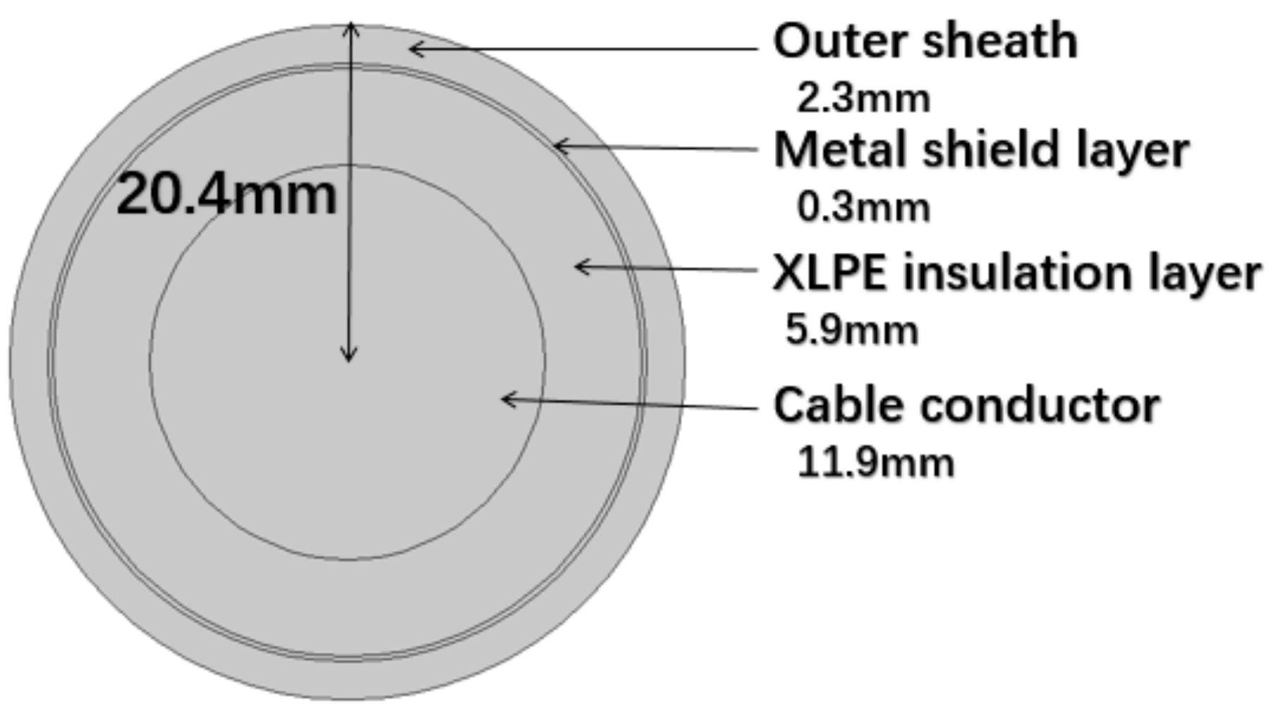
2.1. Physical and Environmental Parameters
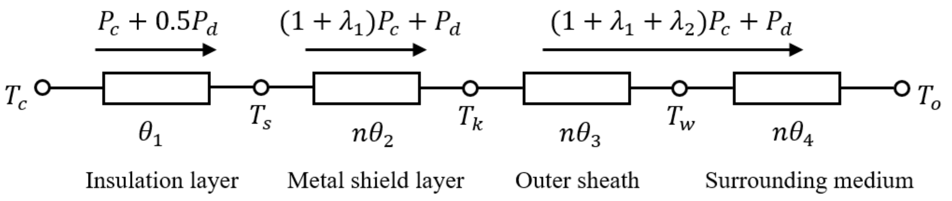
2.2. IEC-60287 Thermal Circuit Method
2.3. Numerical Calculation Method
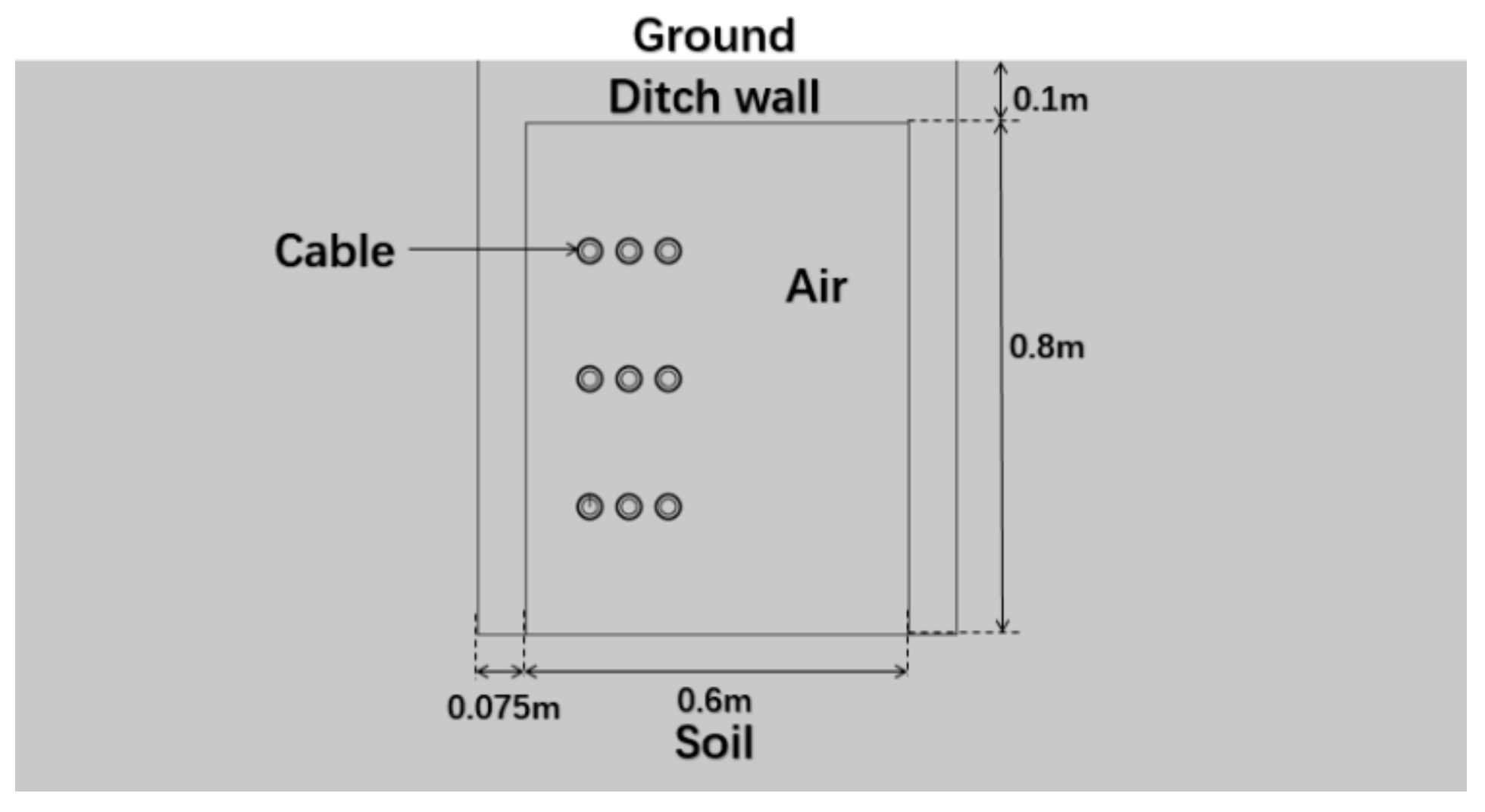
2.3.1. Model of Cable Trench
- (1)
- The steady state temperature field distribution of cable trench is simulated only.
- (2)
- The material properties of the cable and cable trench environments are all isotropic homogeneous media, and the physical properties of materials are constant.
- (3)
- Only the balanced operation of the cables is considered.
- (4)
- The metal shield or sheath layer of the cable is grounded at a single point, without considering the circulation loss of the shield layer.
2.3.2. Heat Transfer Equation
- (1)
- The heat transfer differential equation of the area containing heat source (including cable core, insulating dielectric layer, and shielding layer) is as follows.is the temperature at the point (x, y) in the domain, °C.is the unit volume calorific rate, .is thermal conductivity, .
- (2)
- The heat transfer differential equation of the area without heat source (including other cable layers, soil, cable trench wall, etc.) is as follows.
2.3.3. Boundary Condition
- (1)
- Constant boundary temperature.
- (2)
- Normal heat flow conditions with constant boundary normal heat flux density.
- (3)
- The convective heat transfer conditions in the interface between solid and fluid, occurring when the temperature of the fluid and the convective heat dissipation coefficient of the fluid are known.In the formula,is the thermal conductivity, .is a temperature function on the boundary.is heat flux density, .α is convective heat transfer coefficient, °C).is the fluid temperature, °C.and are the integral boundary.
2.4. Thermal Process Analysis of Cable Trench
2.5. Results and Data Analysis
3. Calculation of Cable Trench Temperature Field and Cable Ampacity
3.1. Cable Ampacity Calculation Method
- (1)
- To estimate the current according to the operation condition, we take the estimated value as the first current tentative value , then is calculated. If meets the condition, then is the cable ampacity. Otherwise, turn to step (2).
- (2)
- The second current test value , which is not much different from the estimated value, is selected to calculate . If meets the condition, then is the cable ampacity, otherwise, turn to step (3).
- (3)
- We take and into formula (7) to get and calculate . If meets the condition, then is the cable ampacity. Otherwise, turn to step (4).
- (4)
- , , , , turn to step (3).
3.2. The Simulation of Temperature Field Distribution
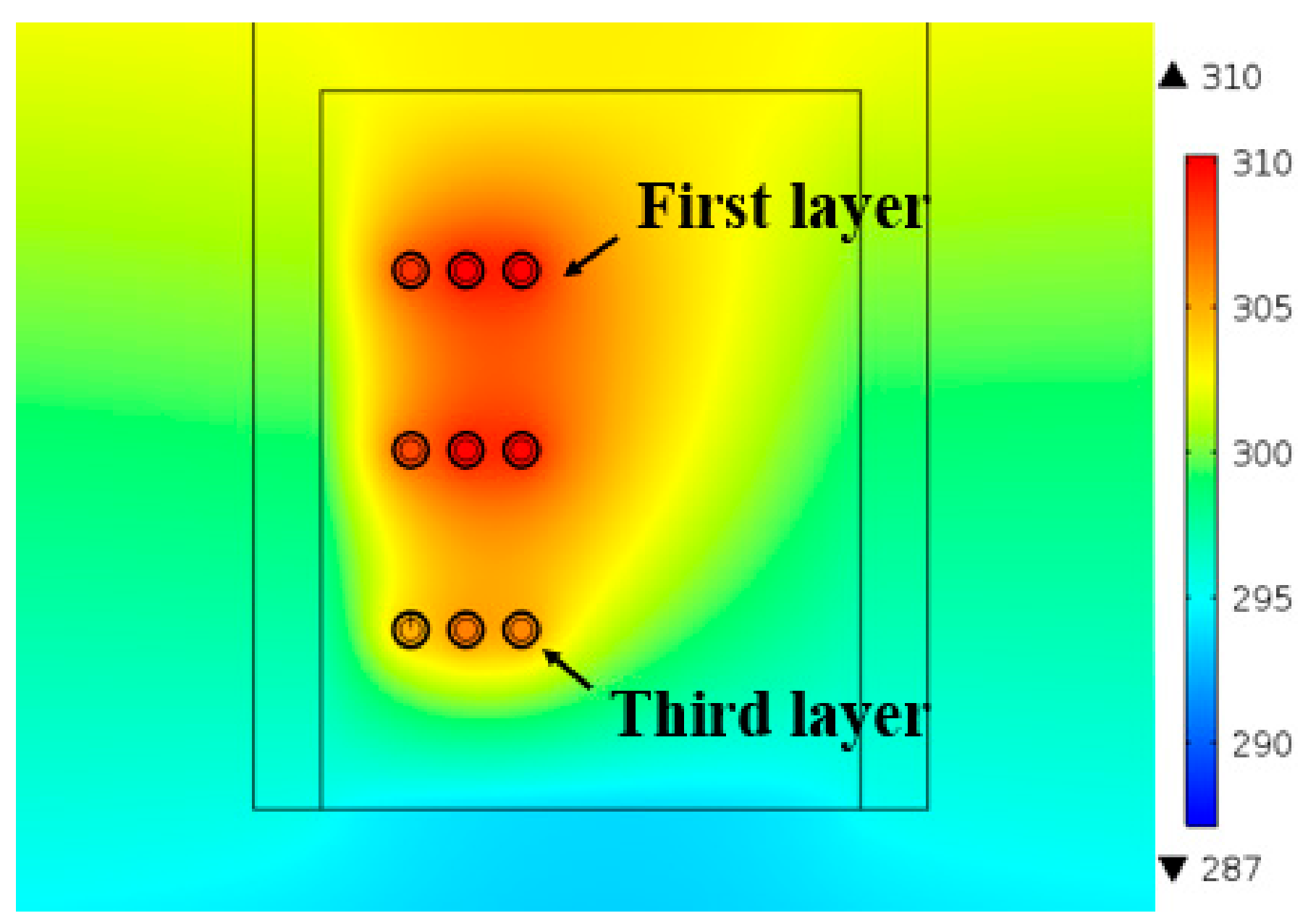
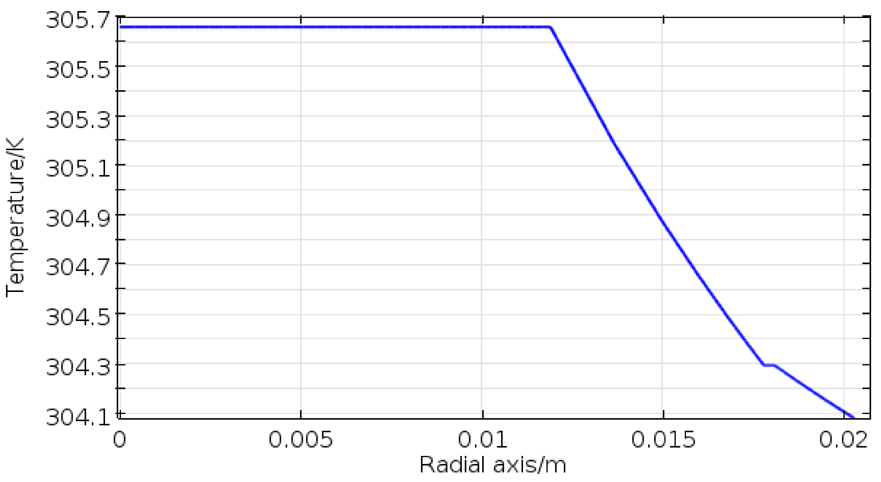
3.2.1. Regular Laying Cables
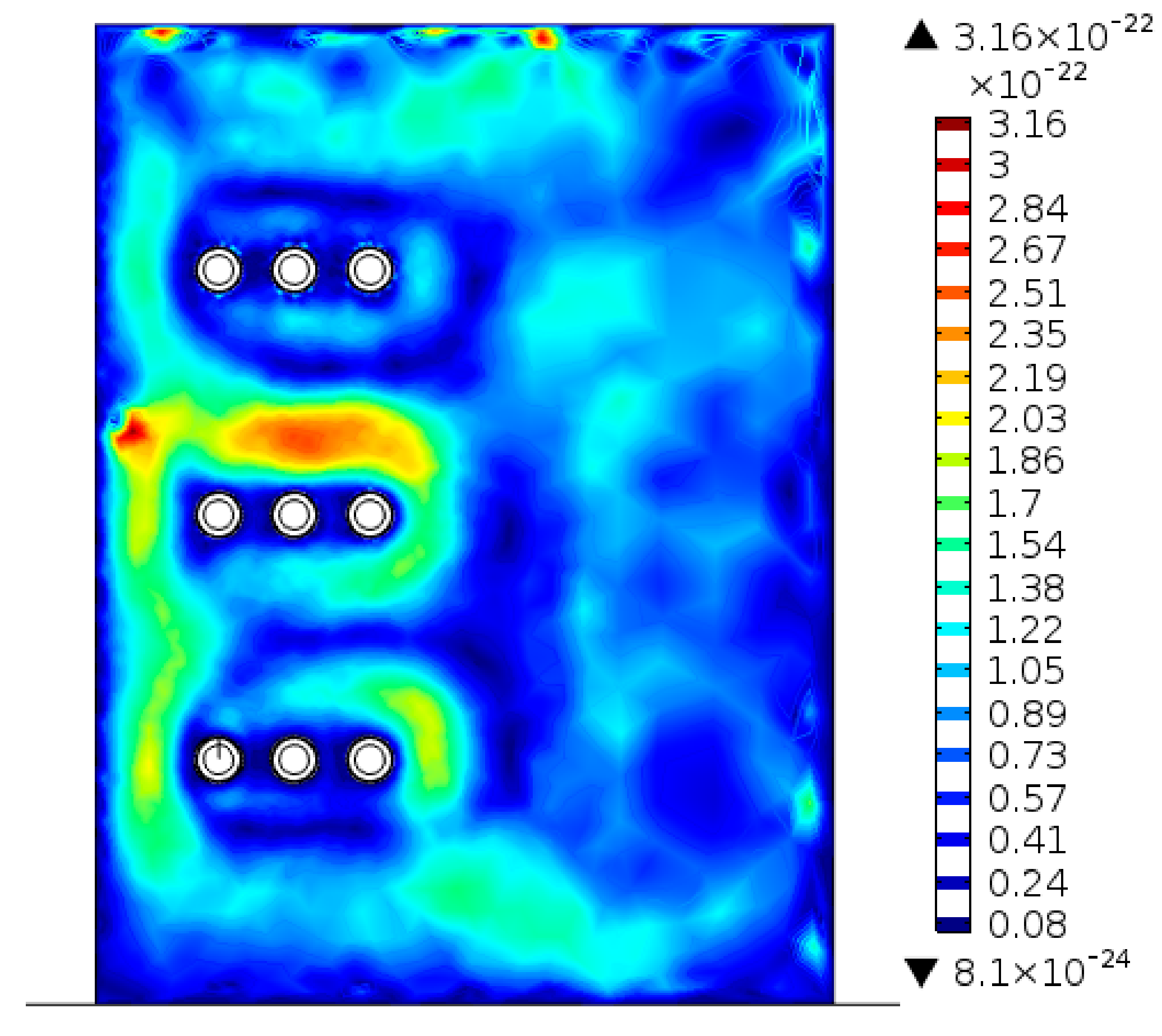
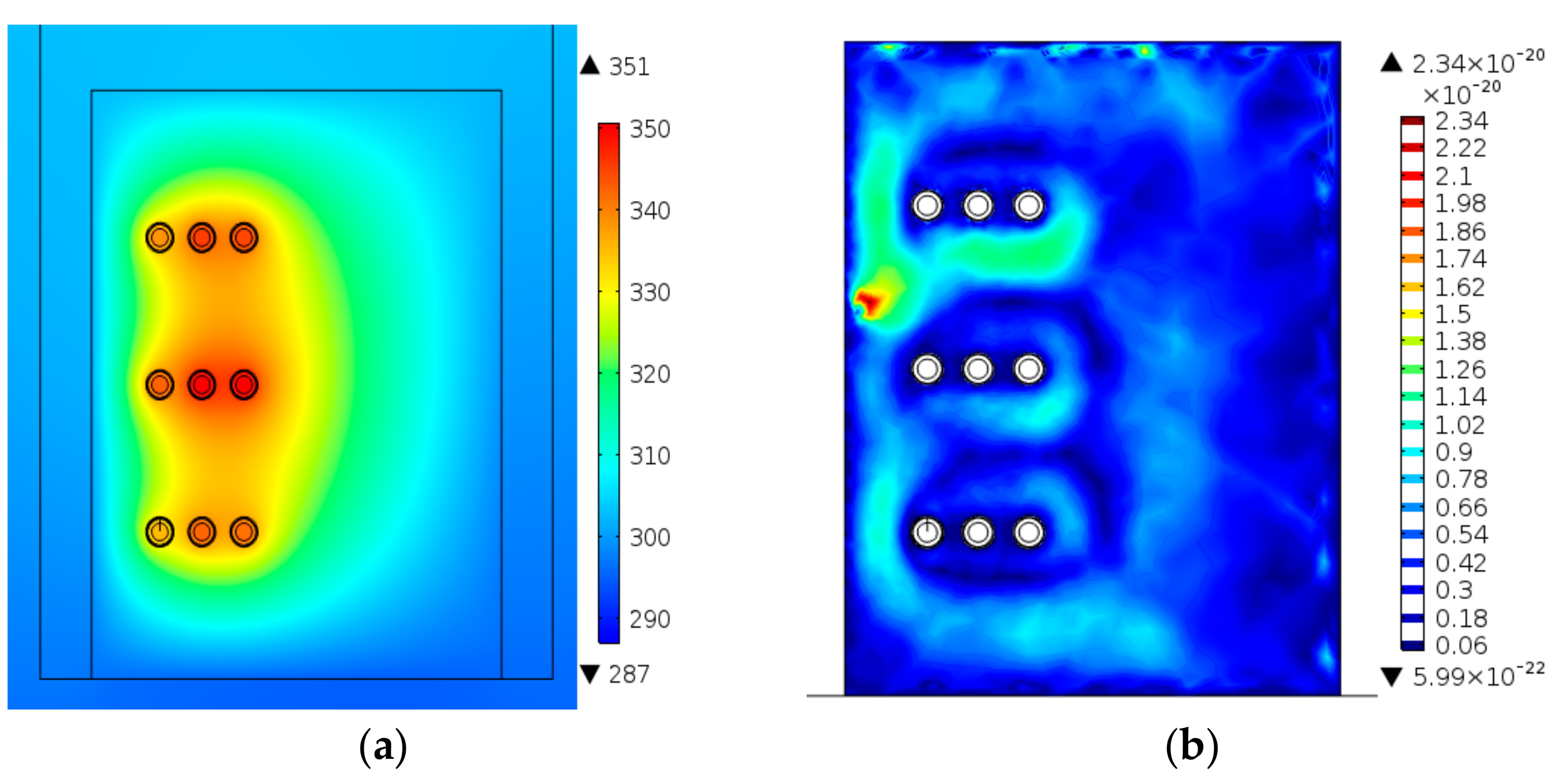
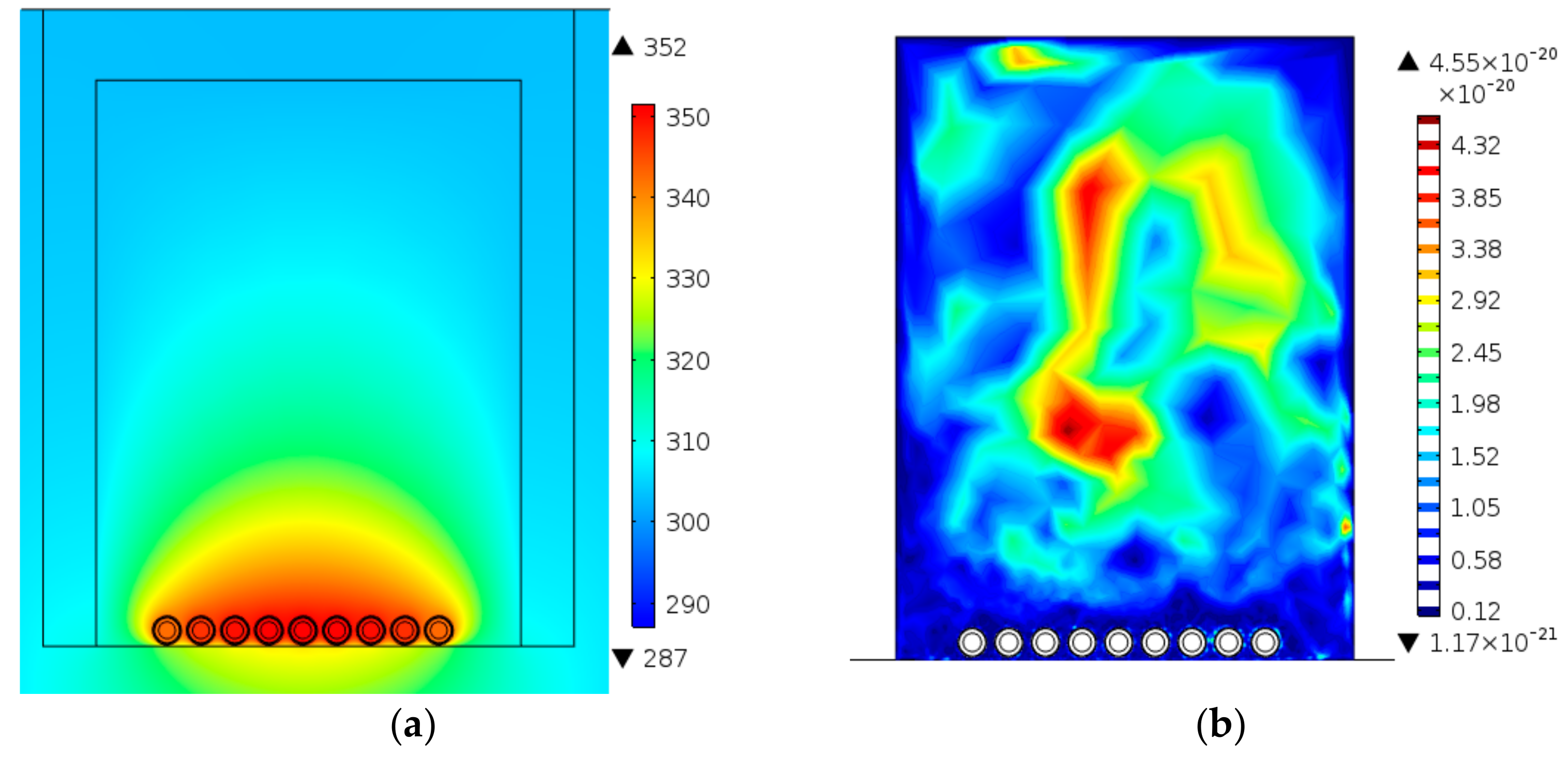
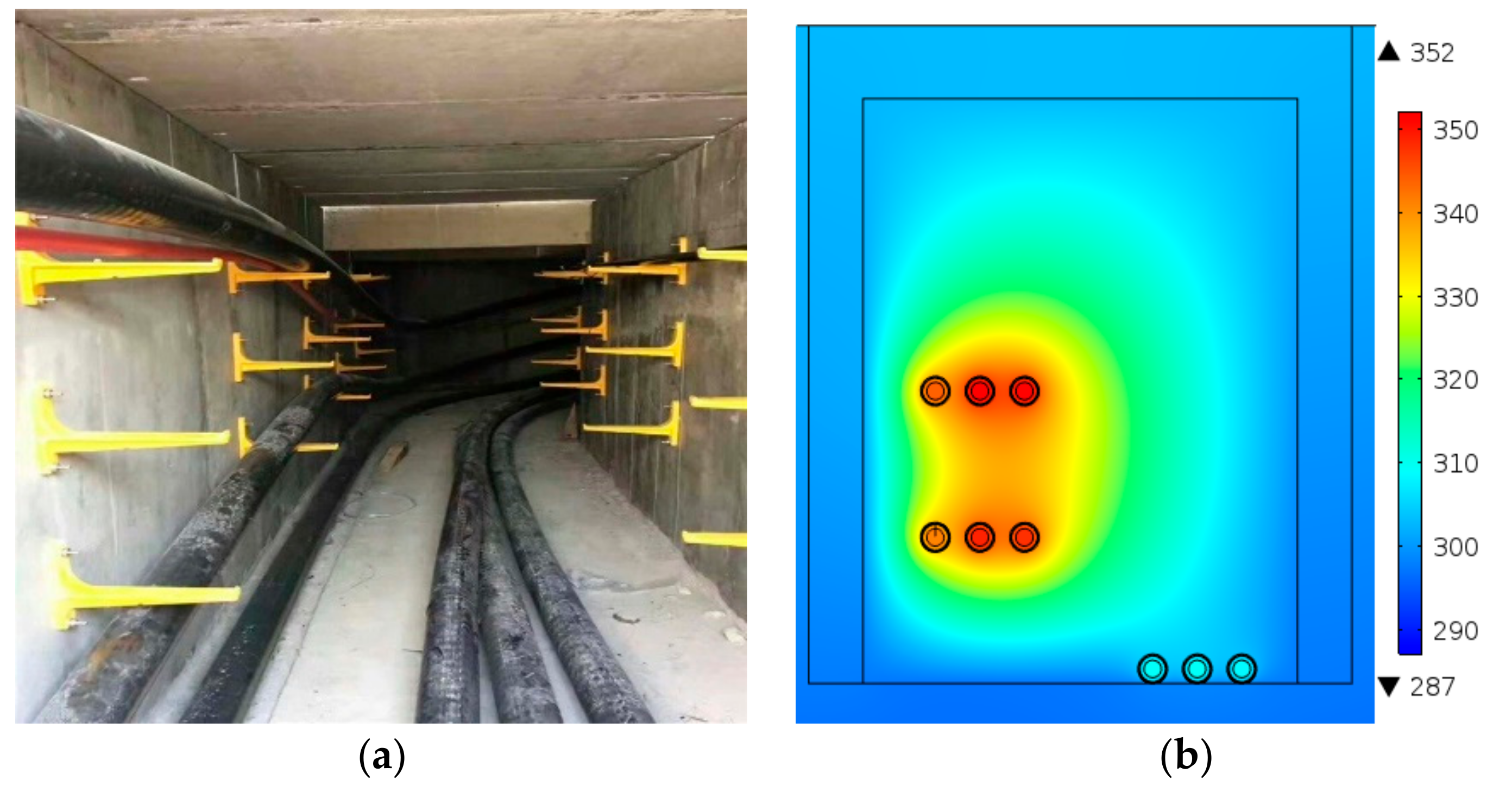
3.2.2. Irregular Laying Cables
4. Online Monitoring System
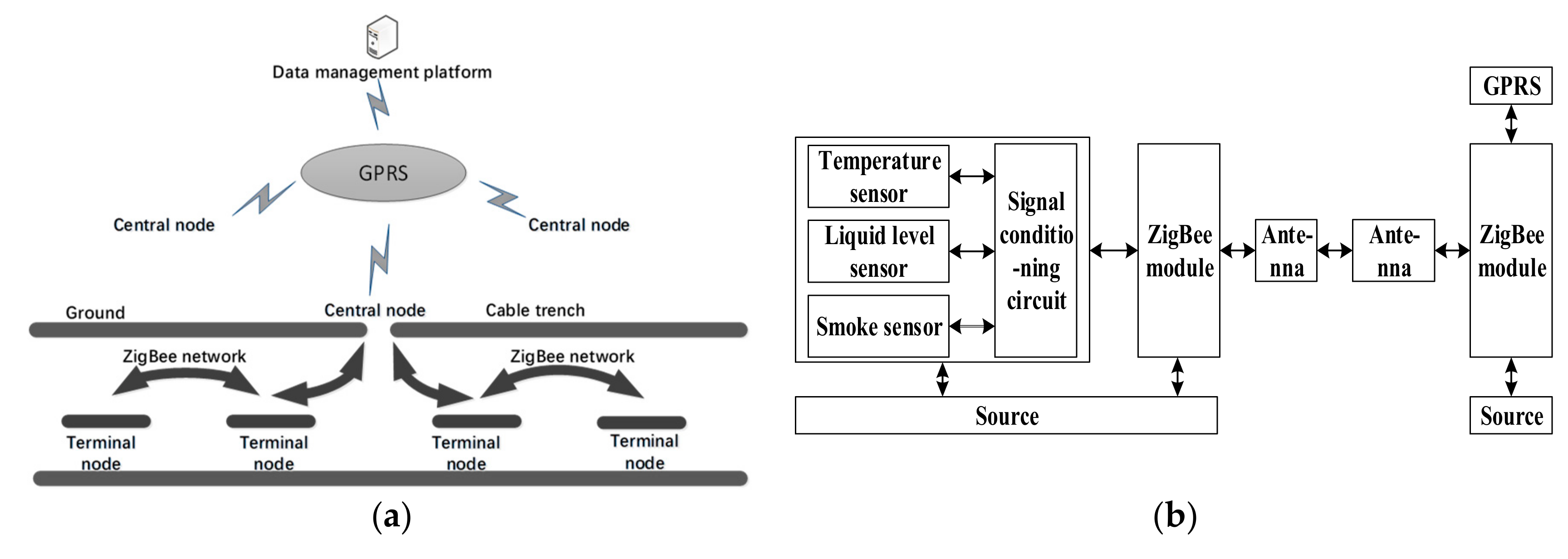
4.1. System Overview
4.2. Program Design and Implementation of Monitoring System
4.3. System Performance Testing
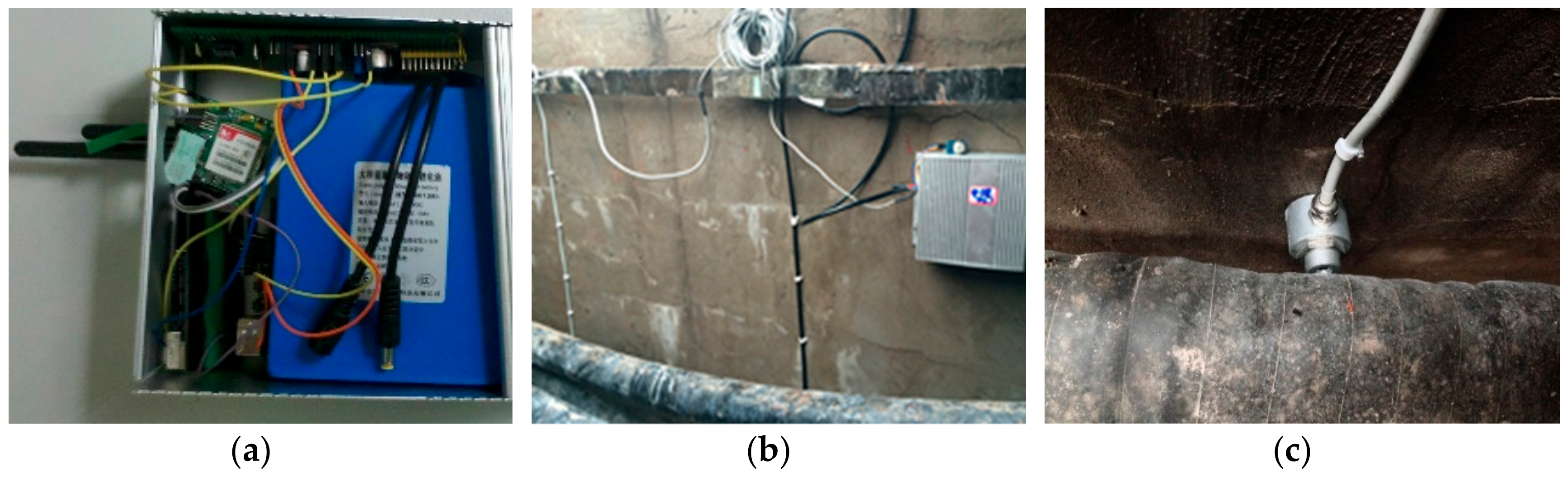
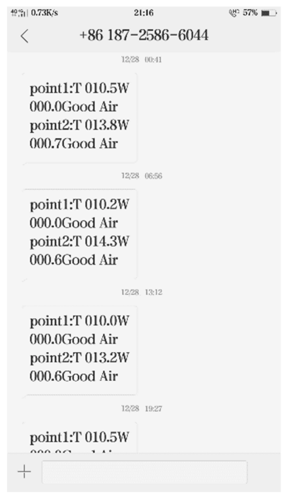
4.4. Application of Monitoring System
5. Discussion
- (1)
- For regular laying cable trenches, the simulated temperature field distribution with different structures has been proposed by many existing literatures, but the simulation error is relatively large, or the overall temperature field inside cable trenches has not been showed, only the temperature distribution curves of a row of cables were given. In this paper, the cable body temperature is obtained by IEC60287 thermal circuit method and numerical calculation method, the error is 0.32%, which can fully meet the actual requirements of the project. In addition, the temperature field and velocity field of the whole cable trench are analyzed.
- (2)
- For irregularly laying cable trenches, few reports can be found in the existing literature. However, the irregular laying of cables is common in field, which may lead to unstable operation and even causes fire in cable trenches. In this paper, the conclusion about both simulation analyses of irregularly laid cables and the calculation of cable current carrying capacity are helpful to standardize the construction of cables.
- (3)
- An online monitoring system is developed to detect timely the highest temperature of cables through simulation analysis, which effectively reduce the number of sensors. Infrared temperature sensors and zigbee are applied with low cost and easy to be installed.
6. Conclusions
- (1)
- Numerical calculation method is more accurate than traditional analytical method in calculating the temperature of cable core based on the temperature of cable skin. The relative error of numerical method is 0.32% and that of the analytical method is 2.3%.
- (2)
- According to the result of steady-state temperature field simulation for the triple-loop cable trench, when the current is small, the hottest point is the core of the first layer cable, and when the current is large, the highest temperature is in the middle layer cable.
- (3)
- Cable laying mode greatly affects the cable ampacity. When the cable cluster is laid at the bottom, the cable ampacity is less than that of regular three-layer cables. The regular mode can reduce the working temperature and prolong the service life of the cable. The higher the density of the cable cluster, the lower the cable ampacity.
- (4)
- An online monitoring system for working environment of power cable is developed. It monitors the temperature of cable, water level in ditch and smoke concentration comprehensively, as to warn faults quickly.
Author Contributions
Funding
Conflicts of Interest
References
- International Electro Technical Commission. IEC 60287-1. Calculation of Current Rating Part 1: (100% Load Factor) and Calculation of Losses; IEC: Geneva, Switzerland, 2001. [Google Scholar]
- Shen, M. Numerical analysis of temperature field in a thawing embankment in per. Can. Geotech. J. 2011, 25, 163–166. [Google Scholar] [CrossRef]
- Lianghua, Z.; Jianjian, Y.; Xiaohu, Z.; Zhiwei, L. A new method for calculating the current carrying capacity and steady-state temperature field of directly buried cables. High Volt. Technol. 2010, 11, 2833–2837. [Google Scholar]
- Yongchun, L.; Yanming, L.; Jinai, C.; Zhenggang, W.; Zhongkui, L. A new method for calculating steady-state temperature field and carrying capacity of underground cable group. J. Electr. Technol. 2007, 22, 185–190. [Google Scholar]
- Youyuan, W.; Rengang, C.; Weigen, C.; Jin, T.; Yuan, Y. Cable current carrying capacity calculation under cable trench laying mode and its influencing factors analysis. Power Autom. Equip. 2010, 30, 24–28. [Google Scholar]
- Ruan, J.; Zhan, Q.; Tang, L.; Tang, K. Real-Time Temperature Estimation of Three-Core Medium-Voltage Cable Joint Based on Support Vector Regression. Energies 2018, 11, 1405. [Google Scholar] [CrossRef]
- Anders, G.J.; Napieralski, A.K.; Kulesza, Z. Calculation of the internal thermal resistance and ampacity of 3-core screened cables with fillers. IEEE Trans. Power Deliv. 1999, 14, 729–734. [Google Scholar] [CrossRef]
- Lee, S.J.; Sung, H.J.; Park, M.; Won, D.; Yoo, J.; Yang, H.S. Analysis of the Temperature Characteristics of Three-Phase Coaxial Superconducting Power Cable according to a Liquid Nitrogen Circulation Method for Real-Grid Application in Korea. Energies 2019, 12, 1740. [Google Scholar] [CrossRef]
- Sedaghat, A.; De Leon, F. Thermal Analysis of Power Cables in Free Air: Evaluation and Improvement of the IEC Standard Ampacity Calculations. IEEE Trans. Power Deliv. 2014, 29, 2306–2314. [Google Scholar] [CrossRef]
- Boshan, Z.; Qingzhu, W. Real-time Conductor’s Temperature Calculation of High Voltage Cable and Prediction 409 Probe of Ampacity. Electr. Eng. 2017, 3, 10–15. [Google Scholar]
- Anders, G.J.; Brakelmann, H. Rating of underground power cables with boundary temperature restrictions. IEEE Trans. Power Deliv. 2017, 33, 1895–1902. [Google Scholar] [CrossRef]
- Yongchun, L.; Yanming, L.; Yanmu, L.; Zhenggang, W.; Zhongkui, L. Numerical methods for transient temperature field and short-term current carrying capacity of underground cables. J. Electr. Technol. 2009, 24, 34–38. [Google Scholar]
- Youyuan, W.; Rengang, C.; Weigen, C.; Jin, T.; Yuan, Y. Finite element method for calculating steady-state temperature field of underground cables and its influencing factors. High Volt. Technol. 2009, 12, 3086–3092. [Google Scholar]
- Yildiz, Ş.; İnanir, F.; Çiçek, A.; Gömöry, F. Numerical study of AC loss of two-layer HTS power transmission cables composed of coated conductors with a ferromagnetic substrate. Turk. J. Electr. Eng. Comput. Sci. 2017, 25, 3528–3539. [Google Scholar] [CrossRef]
- Garrido, C.; Otero, A.F.; Cidras, J. Theoretical model to calculate steady-state and transient ampacity and temperature in buried cables. IEEE Trans. Power Deliv. 2003, 18, 667–678. [Google Scholar] [CrossRef]
- Doukas, D.I.; Chrysochos, A.I.; Papadopoulos, T.A.; Labridis, D.P.; Harnefors, L.; Velotto, G. Volume element method for thermal analysis of superconducting DC transmission cable. IEEE Trans. Appl. Supercond. 2017, 27, 1–8. [Google Scholar] [CrossRef]
- Haiqing, N.; Wenjian, Z.; Chaoping, L.; Kaifa, Y.; Yong, W.; Guojun, L. Estimation method of soil thermal parameters around cables based on finite element method and particle swarm optimization. High Volt. Technol. 2018, 44, 1557–1563. [Google Scholar]
- De Leon, F. Major factors affecting cable ampacity. In Proceedings of the 2006 IEEE Power Engineering Society General Meeting, Montreal, QC, Canada, 18–22 May 2006. [Google Scholar]
- Bates, C.; Malmedal, K.; Cain, D. Cable Ampacity Calculations: A Comparison of Methods. IEEE Trans. Ind. Appl. 2016, 52, 112–118. [Google Scholar] [CrossRef]
- Shabagin, E.; Heidt, C.; Strauß, S.; Grohmann, S. Modelling of 3D temperature profiles and pressure drop in concentric three-phase HTS power cables. Cryogenics 2017, 81, 24–32. [Google Scholar] [CrossRef]


| Cable Structure | mm |
|---|---|
| Inner radius of cable | 11.9 |
| Insulation width | 5.9 |
| Metal shield width | 0.3 |
| Outer sheath width | 2.3 |
| Outer radius of cable | 20.4 |
| Laying Environment | Parameter Values |
|---|---|
| Soil thermal resistance/ | 23.8 |
| Air temperature/ | 313 |
| Deep soil temperature/ | 293 |
| Ditch wall thermal conductivity/ | 1.73 |
| Bracket thermal conductivity/ | 44.5 |
| Cable Serial Number | 200 A/K | 481 A/K |
|---|---|---|
| 1 | 308.66 | 338.54 |
| 2 | 310.28 | 345.48 |
| 3 | 310.16 | 344.77 |
| 4 | 308.08 | 342.43 |
| 5 | 309.98 | 350.80 |
| 6 | 309.92 | 350.60 |
| 7 | 305.68 | 335.44 |
| 8 | 306.42 | 342.31 |
| 9 | 306.42 | 341.49 |
| Cables at the Bottom | Cable Ampacity/A |
|---|---|
| First layer | 517 |
| Second layer | 542 |
| Third layer | 513 |
| Test Point | Actual Value/°C | Test Value/°C | Relative Error/% |
|---|---|---|---|
| Node 2 | 20.2 | 20.6 | 1.98 |
| Node 2 | 20.8 | 21.2 | 1.92 |
| Node 2 | 21.5 | 21.9 | 1.86 |
| Node 2 | 28.2 | 28.8 | 2.12 |
| Node 2 | 28.5 | 28.9 | 1.40 |
| Node 2 | 24.8 | 25.2 | 1.61 |
| Node 2 | 24.4 | 24.9 | 2.04 |
| Node 2 | 23.6 | 24.2 | 2.54 |
| Node 2 | 23.5 | 23.9 | 1.70 |
| Node 2 | 23.5 | 23.9 | 1.70 |
| Test Point | Time | Temperature (°C) |
|---|---|---|
| Node 1 | 00:41 | 10.5 |
| 06:56 | 10.2 | |
| 13:12 | 10.0 | |
| Node 2 | 00:41 | 13.8 |
| 06:56 | 14.3 | |
| 13:12 | 13.2 |
© 2019 by the authors. Licensee MDPI, Basel, Switzerland. This article is an open access article distributed under the terms and conditions of the Creative Commons Attribution (CC BY) license (http://creativecommons.org/licenses/by/4.0/).
Share and Cite
Xiong, L.; Chen, Y.; Jiao, Y.; Wang, J.; Hu, X. Study on the Effect of Cable Group Laying Mode on Temperature Field Distribution and Cable Ampacity. Energies 2019, 12, 3397. https://doi.org/10.3390/en12173397
Xiong L, Chen Y, Jiao Y, Wang J, Hu X. Study on the Effect of Cable Group Laying Mode on Temperature Field Distribution and Cable Ampacity. Energies. 2019; 12(17):3397. https://doi.org/10.3390/en12173397
Chicago/Turabian StyleXiong, Lan, Yonghui Chen, Yang Jiao, Jie Wang, and Xiao Hu. 2019. "Study on the Effect of Cable Group Laying Mode on Temperature Field Distribution and Cable Ampacity" Energies 12, no. 17: 3397. https://doi.org/10.3390/en12173397
APA StyleXiong, L., Chen, Y., Jiao, Y., Wang, J., & Hu, X. (2019). Study on the Effect of Cable Group Laying Mode on Temperature Field Distribution and Cable Ampacity. Energies, 12(17), 3397. https://doi.org/10.3390/en12173397