Deep Learning-Based Short-Term Load Forecasting for Supporting Demand Response Program in Hybrid Energy System

Abstract

A novel method for short-term load forecasting (STLF) is proposed in this paper. The method utilizes both long and short data sequences which are fed to a wavenet based model that employs dilated causal residual convolutional neural network (CNN) and long short-term memory (LSTM) layer respectively to hourly forecast future load demand. This model is aimed to support the demand response program in hybrid energy systems, especially systems using renewable and fossil sources. In order to prove the generality of our model, two different datasets are used which are the ENTSO-E (European Network of Transmission System Operators for Electricity) dataset and ISO-NE (Independent System Operator New England) dataset. Moreover, two different ways of model testing are conducted. The first is testing with the dataset having identical distribution with validation data, while the second is testing with data having unknown distribution. The result shows that our proposed model outperforms other deep learning-based model in terms of root mean squared error (RMSE), mean absolute error (MAE), and mean absolute percentage error (MAPE). In detail, our model achieves RMSE, MAE, and MAPE equal to 203.23, 142.23, and 2.02 for the ENTSO-E testing dataset 1 and 292.07, 196.95 and 3.1 for ENTSO-E dataset 2. Meanwhile, in the ISO-NE dataset, the RMSE, MAE, and MAPE equal to 85.12, 58.96, and 0.4 for ISO-NE testing dataset 1 and 85.31, 62.23, and 0.46 for ISO-NE dataset 2.

1. Introduction

Nowadays, the hybrid energy system has become more popular in the electricity industry. The main reason of this trend is the exponential reduction of energy storage cost and the development of digital connection, enabling real time monitoring and smarter grid establishment. Moreover, the hybrid energy system is considered as one of the best solutions in tackling intermittency experienced by most renewable energy schemes including solar- and wind-based energy. For example, in solar photovoltaic, the energy is only delivered when obtaining sufficient solar irradiance. As a consequence, a lot of research has been conducted in order to provide the best scheme of this hybrid system [1].

Among provided hybrid energy system schemes, the most possible way to be implemented in the majority of countries is the integration between renewable and fossil energy, because fossil energy has already well established. In case of sustainability, this scheme is very good, because fossil energy is obviously able to supply adequate power to the grid when the alternative sources cannot handle users’ load demand. The major concern of this scheme is the cost to be borne by users once the renewable sources cannot supply adequate power to the grid in which they will pay an expensive fossil-based electric price. Moreover, fossil energy tends to gradually increase leading to economic conflict in society [2]. Therefore, in order to tackle this issue, an appropriate demand response scheme can be applied.

Demand response is the change of electric usage by users due to change of electric price or maybe an incentive as a reward of lowering their power consumption [3]. Applying demand response to this hybrid system is very beneficial for shaving peak load demand [4,5], leading to the reduction of fossil energy consumption. Moreover, it can provide short-term impact and economic benefit for both consumer and utility.

In order to support this demand response, short-term load forecasting (STLF) is very important for predicting whether the energy storage from renewable sources is able to handle the forthcoming power consumption or not. If the prediction states that the storage is not adequate to support the future load, then the electricity utility can announce this situation to the users, which eventually triggers them to reduce their electric usage, because users do not only want to pay more for conventional energy source but also want to get incentives from the authorities.

Fortunately, with the help of developed infrastructures like smart meters equipped with a lot of sensors and the Internet of Things (IoT), a robust STLF method is feasible to be implemented. Broadly speaking, research in load forecasting can be categorized into two research classes, traditional and advanced model. Traditional model uses simple statistics method for example regression models [6] and Kalman filtering model [7]. Nevertheless, among proposed traditional models, autoregressive integrated moving average (ARIMA) and generalized autoregressive conditional heteroscedascity (GARCH) are two of the most popular techniques in regression function that were used in several precedent research studies [8,9]. Unfortunately, these traditional models only provide good accuracy if the electrical load and other parameters have a linear relationship. Meanwhile, the advanced model is a data-driven model implementing the machine learning technique for instance support vector machine (SVM) [10], K-nearest neighbor (KNN) [11], and others [12,13,14].

However, based on the recent publications [15,16,17,18], the deep learning-based methods show the most convincing performance by outperforming other machine learning-based solutions. The main reason of the deep learning superiority is first, deep learning does not highly rely on feature engineering and the hyperparameters tuning is relatively easier compared to other data-driven models. The second is the availability of huge datasets, where deep learning can precisely map the inputs to the certain output by making complex relations among layers in the network based on that huge training data. Moreover, since the availability of Graphics Processing Unit (GPU) parallel computation and methods providing weights sharing like convolutional neural network (CNN) [19], the computational speed of deep learning models become significantly faster.

Because of the superiority of the deep learning, this research proposes a method in load forecasting task, specifically STLF, to predict the hourly power consumption by using deep learning algorithms which is the combination of the advanced version of the convolutional neural network (CNN), dilated causal residual CNN, and long short-term memory (LSTM) [20].Dilated causal residual CNN is inspired by the Wavenet model [21], which is very famous for audio generation, and the residual network [22] with gated activation function. This model will learn the trend based on long sequence input while the LSTM layer works as a model’s output self-correction which relates the output of the wavenet-based model with the recent load demand trend (short sequence).

The main contribution of this research is that we propose a novel model utilizing a combination of dilated causal residual CNN and LSTM utilizing long and short sequential data and fine tuning technique. External feature extraction or feature selection data are not included in this research. Moreover, this research only takes into account time index information as the external factor data, making it easy to be compared as a benchmark model for future research.

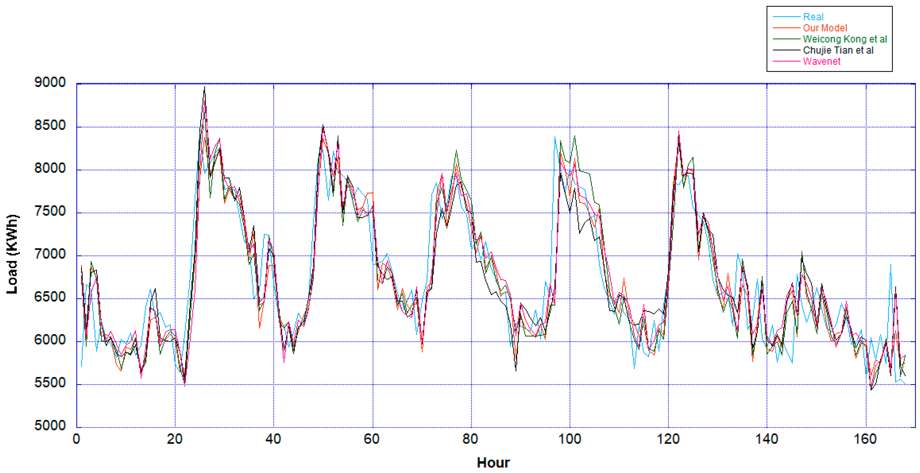
In order to prove the generality of our proposed model performance, two different scenarios of model testing are conducted. The first scenario is using the testing dataset having identical distribution with the validation dataset, while the second is using dataset having unknown distribution. As a comparison, our proposed model results are compared with the performance of the model from [15,16] and the standard wavenet [21]. The simulation result shows that our proposed model outperforms other deep learning models in root mean squared error (RMSE), mean absolute error (MAE), and mean absolute percentage error (MAPE).

Therefore, due to the accuracy of our model performance, this model can be used for supporting utilities in applying demand response program since it can help the utilities to obtain accurate prediction about the future load demand that eventually providing precise information to the users whether the future load demand can be supplied by the renewable source or not.

The rest of the paper is organized as follows. Section 2 describes the dataset used in detail including preliminary data analysis and data preprocessing. Section 3 explains the model architecture and its parameter, training, and testing stage. Section 4 provides information about results obtained by using the proposed models compared with other deep learning-based models and clear explanation about the reason why the proposed model can achieve the result. Lastly, Section 5 summarize the findings discussed in this paper and also possible future works.

2. Dataset

In order to prove the generality of our proposed method, two datasets are used as the model’s input which are the ENTSO-E (European Network of Transmission System Operators for Electricity) [23] and ISO-NE (Independent System Operator New England) dataset [24]. The ENTSO-E dataset is the dataset obtained from load demand in every country in Europe. In this research we only take into account data gathered from Switzerland. Meanwhile, the ISO-NE dataset is data of hourly load demand in New England.

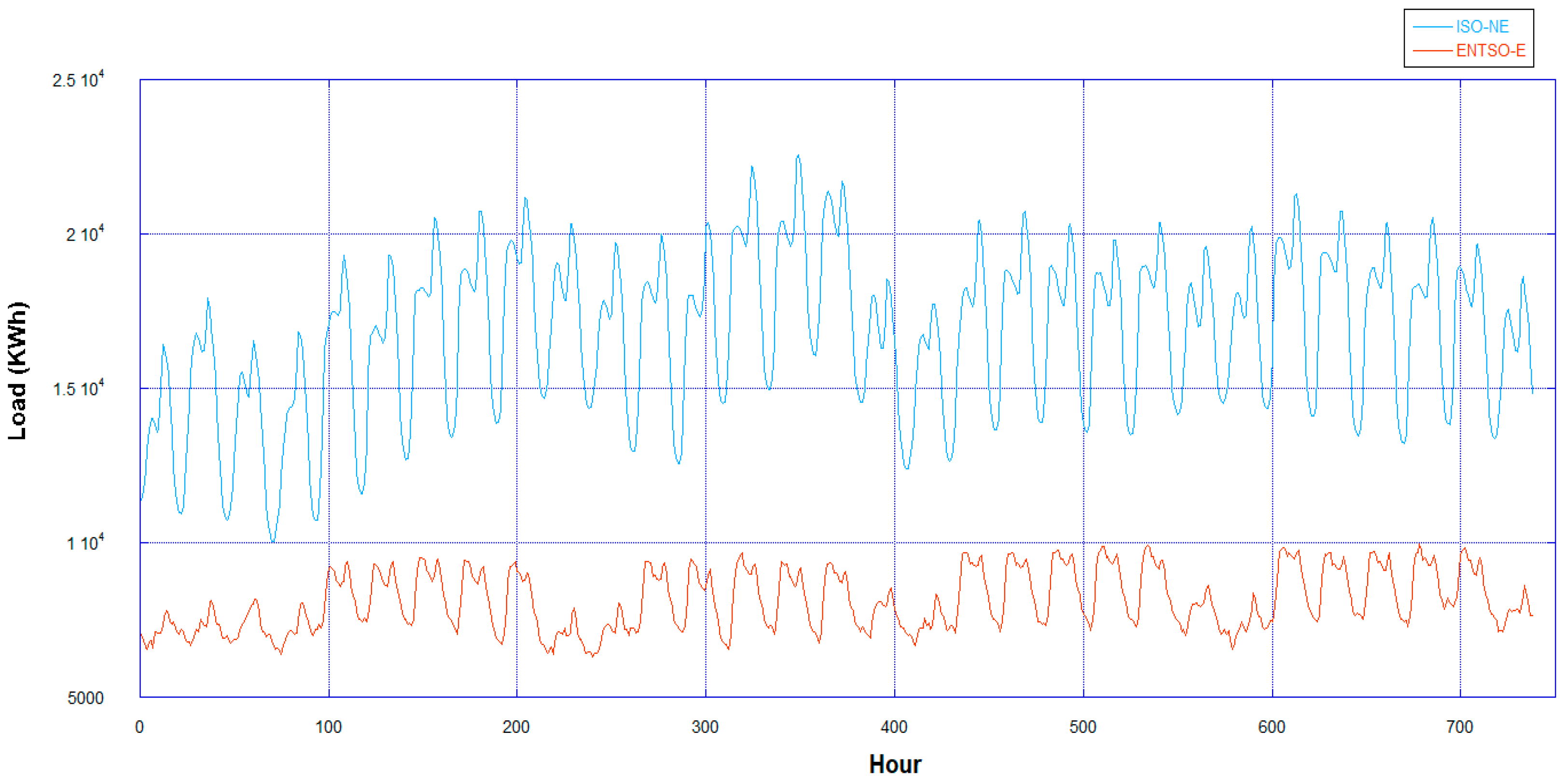
Those datasets have different kinds of characteristics, especially in the case of load demand range and complexity. In the ENTSO-E dataset, the lowest and highest value of load are 1483 KWh and 18,544 KWh, respectively, while in the ISO-NE dataset they are 9018 KWh and 26,416 KWh, respectively. Another different characteristic is the fluctuation trend in a single day load demand. In the ENTSO-E dataset, the load demand is more oscillated compared to the ISO-NE dataset. As proof, Figure 1 and Figure 2 show the average daily power consumption and example of load trend in a day based on those datasets and example of demand trend of each dataset.

In building a solution for load forecasting, deep understanding of the load demand trend is very necessary. Figure 3 shows data in both datasets over a year period. From Figure 3, broadly speaking, the trend of load demand has a periodicity that will be repeated over the next weeks. However, this trend is highly affected by a lot of external factors causing a fluctuation over a certain period, for example, the economic, weather, and time index. Unfortunately, obtaining those external factors are difficult, the easiest external data that can be gathered is time index data containing information about the date and clock. Therefore, in this research we not only fed the model by load demand trend but also time index data represented by one-hot vector. One-hot vector is a sparse vector that maps a feature with M categories into a vector which has M elements where only the corresponding element is one while the remaining are zero.

Before fed to the model, the datasets must be pre-processed, which consists of checking for null values, splitting dataset into training, validation and testing dataset, and eventually data normalization. The data used for this research is limited only to data taken from 1 January 2015 until 30 May 2017 for the ENTSO-E dataset and from 1 January 2004 until 30 May 2006 for the ISO-NE dataset. The first two years of data are used for the training stage, while the rest of the 3600 data are split into 3000 and 600 data. The first 3000 data are randomly taken for validation and testing data with proportion of nearly 0.65 and 0.35 to be used for validation and the testing stage, respectively. In other words, the total of validation data and first testing data are 1900 and 1100, respectively, while another 600 data are used for the second testing data. We conduct two testing stage, because the first testing data have a nearly identical distribution with the validation data which clearly make the model provide good accuracy in the testing stage. Meanwhile, the second testing data is clearly new data that their distribution is never experienced by the model both in the training and validation stage. This kind of testing process is appropriate for proving the generality of the model.

In the data normalization process, min-max scaling method as expressed in Equation (1) is implemented.

$$z_i=\frac{x_i-\min \left(x\right)}{\max \left(x\right)-\min \left(x\right)}$$

(1)

$x= x_1,\dots , x_n$ and $z_i$ is the i^th normalized data. The parameters in the normalization process must come from training dataset only, because we assume that the future data (validation and test set) have different distribution with the training dataset.

3. Model Design

In this research, the cores of the proposed model are wavenet architecture implementing both of the dilated causal CNN and residual network and LSTM, which have proven very well in time-series data prediction.

Our proposed model consists of two stages that have a function to learn long and short sequence data. Inspired by the success of wavenet architecture and LSTM in handling time series data, the long sequence taken from the 32 time steps before the target is learned using wavenet while the short sequence taken from 4 time steps before target is learned using LSTM.

3.1. Wavenet

Wavenet consists of deep generative models utilizing the dilated causal convolutional neural network of audio waveform. Causal convolution means that the output of the recent time step is only affected by the previous time step. Meanwhile, the dilated convolutional neural network is a modified convolutional neural network where the filter weight alignment is expanded by a dilation factor that eventually results in a broader receptive field that can be expressed as follows:

$$\left(F{\ast }_{l}k\right)\left(\mathit{p}\right)={\displaystyle \sum }_{s+l\mathit{t}=\mathit{p}}F\left(s\right)k\left(\mathit{t}\right)$$

(2)

while the standard convolution is expressed as follows:

$$\left(F\ast k\right)\left(\mathit{p}\right)={\displaystyle \sum }_{s+\mathit{t}=\mathit{p}}F\left(s\right)k\left(\mathit{t}\right)$$

(3)

The dilated convolution is denoted by ${\ast }_l$ notation. The difference between dilated convolution with standard convolution is the notation $l$ representing the dilation factor which causes the filter to skip one or several points during the convolution process.

Figure 4 shows the dilated convolution applied in one dimensional data. The blue, white, and orange circle are input data, hidden layer output, and output layer output, respectively. There are 32 input data taken from t = 1 until t = 32 that are convoluted with filter with the size of two. The dilation rate is increased by one in every hidden layer that causes a broader receptive field. This dilation rate is repeated twice. In the output layer, only the last value is taken, which we assume represents the feature of load at t = 33.

In order to optimize the usage of the dilated convolutional neural network, the residual technique [22] is applied to the model. The implementation of the residual network will take into account lower levels outputs which have features that will help in predicting the future power demand, especially in the case of a network implementing a sparse filter which has the potential to lose several information from the previous layers.

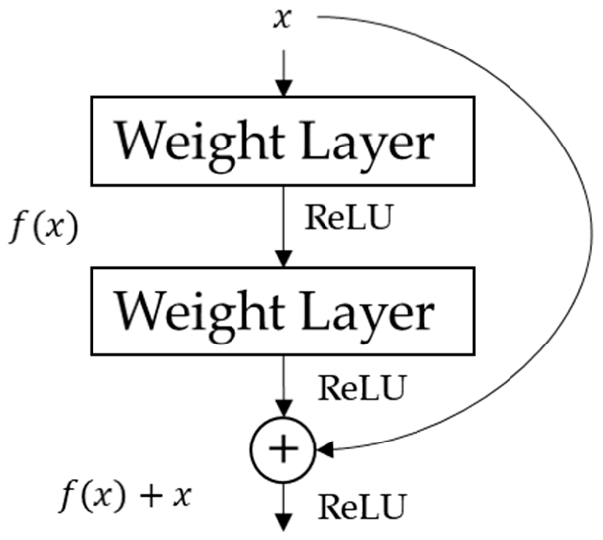
The residual model is a famous way to build the deep neural network that was firstly proposed for the image recognition task. Using this way, instead of only mapping input data $x$ to a function $H\left(x\right)$ that outputs $\widehat{y}$, the mapping scenario from the previous residual block $f\left(x,\left\{W_i\right\}\right)$ where $W_i$ is the learned weights and biases from the residual block i is also considered. Therefore, the output of the residual block can be expressed as:

$$H\left(x\right)=f\left(x,\left\{W_i\right\}\right)+x$$

(4)

Moreover, since we use the stacked residual block, then the output of the residual block can be represented as:

$$x_K=x_0+{\displaystyle \sum }_{i=1}^{K}f\left(x_{i-1},W_{i-1}\right)$$

(5)

$x_K$ is the output of residual block K, $x_0$ is the input of the residual network and $f\left(x_{i-1},W_{i-1}\right)$ is the output and associated weight of the previous residual blocks. As a result of several summation between the previous and final residual block, then the back propagation of the network to $x_0$ can be calculated using the following equation:

$$\frac{\partial ℒ}{\partial x_0}=\frac{\partial ℒ}{\partial x_K}\frac{\partial x_K}{\partial x_0}=\frac{\partial ℒ}{\partial x_K}\left(1+\frac{\partial }{\partial x_0}{\displaystyle \sum }_{i=1}^{K}f(x_{i-1},W_{i-1})\right)$$

(6)

$ℒ$ is the total loss of the network and constant 1 indicates that the gradient of the network output can be directly back-propagated without considering layers’ parameters (weights and biases). This formulation ensures the layers do not suffer of vanishing gradient, even the weights are small. Figure 5 shows the basic residual learning process.

Moreover, skip connection and gated activation are applied to the network for speeding up the convergence and avoiding overfitting. The process of residual and skip connection with gated activation is shown in Figure 6.

The gated activations are inspired by the LSTM layer where tanh and sigmoid $\left(\sigma \right)$ work as learned filter and learned gate, respectively. The use of gated activations has been proved to work better compared to using ReLU activation in time series data [21]. The output of dilated convolution with gated activations can be expressed as:

$$z=\tanh \left(w_f\ast x\right)\odot \sigma \left(w_g\ast x\right)$$

(7)

where $w_f$ and $w_g$ are learned filter and learned gate, respectively.

3.2. LSTM

In the case of forecasting future data, the knowledge of the recent trend is very essential. As an illustration, in predicting future data, we mostly start to figure out a long sequence trend. After we have already known the pattern of the trend based on the long sequence of previous data, then in order to provide better forecast, we also try to relate our understanding of long sequence data with the recent trend. The same concept is applied to our proposed method. We fine tune the wavenet-based model with one LSTM layer assigned to help the network to relate the output of dilated CNN with the recent trend. This step can also be considered as a correction step of the dilated CNN output, as we assert a fix input to be concatenated with dilated CNN output which are then fed to the LSTM layer that also work as output layer.

Brief Explanation of LSTM

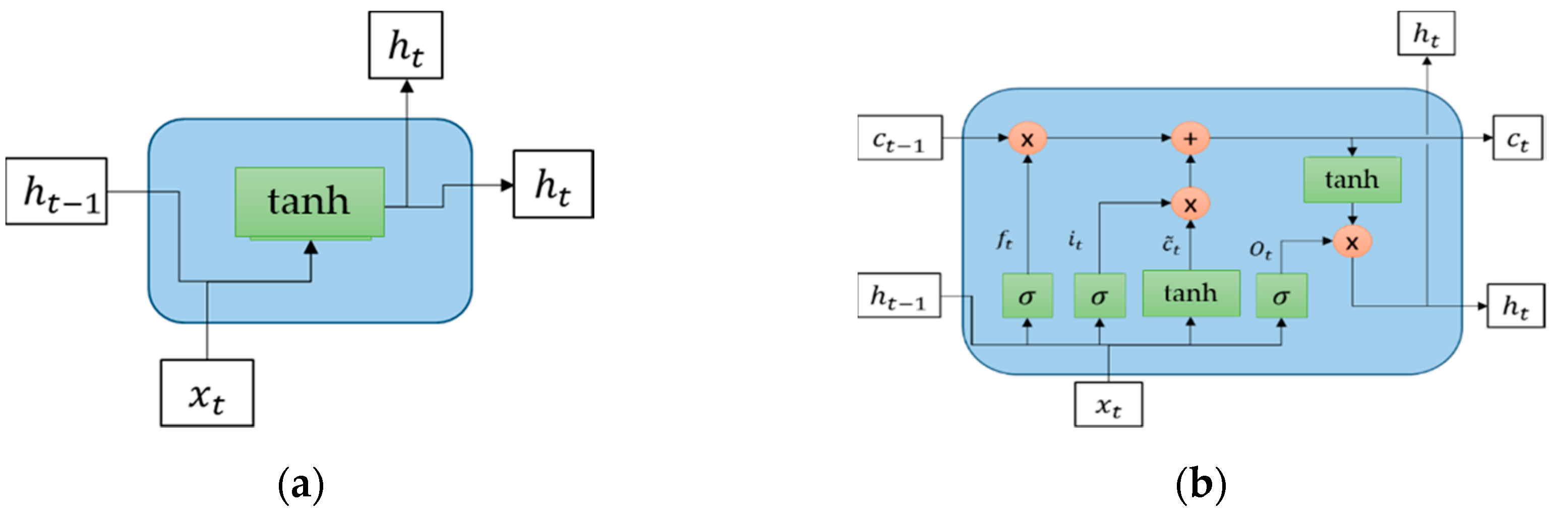
LSTM is the developed version of the standard recurrent neural network (RNN) where instead of only having a recurrent unit, LSTM has “LSTM cells” that have an internal recurrence consisting of several gating units controlling flow of information [25]. Comparison between the simple RNN and LSTM layer using tanh as the activation function is depicted in Figure 7.

From Figure 7, the difference between the simple RNN and LSTM layer is clear. The LSTM layer is more complex than the simple RNN, because LSTM not only takes into account input ($x$) and hidden state ($h$) at a certain time step, but also LSTM cells ($c$) that will replace the hidden state to prevent older signals from vanishing during the process. Three control gates ruling the LSTM cells, forget gate, input gate, and output gate are represented by $f_{t,}$ $i_t$, $O_t$, respectively. Those gates use sigmoid activation function having an output range between 0 and 1 represented by $\mathsf{\sigma }$. Meanwhile, ${\tilde{c}}_t$ is the input node that works identical to the simple RNN layer.

Mathematically explained, forget gate and input gate, respectively can be expressed as:

$$i_t = \sigma \left(W_i\times \left[h_{t-1},x_t\right]+b_i\right)$$

(8)

$$f_t = \sigma \left(W_f\times \left[h_{t-1},x_t\right]+b_f\right)$$

(9)

$\left[h_{t-1},x_t\right]$ is the concatenation between input and hidden state value, while $W$ and $b$ are weight matrices, respectively. On the other hand, the cell state is updated with the formulation:

$$c_t = f_t\times c_{t-1}+i_t\times {\tilde{c}}_t$$

(10)

where ${\tilde{c}}_t$ is expressed as:

$${\tilde{c}}_t=\tanh \left(W_c\times \left[h_{t-1},x_t\right]+b_c\right)$$

(11)

The last, the output gate $o_t$ and hidden state $h_t$ is calculated by using the following equation:

$$o_t = \sigma \left(W_o\times \left[h_{t-1},x_t\right]+b_o\right)$$

(12)

$$h_t=o_t\times \tanh \left(c_t\right)$$

(13)

3.3. Detailed Model Setup

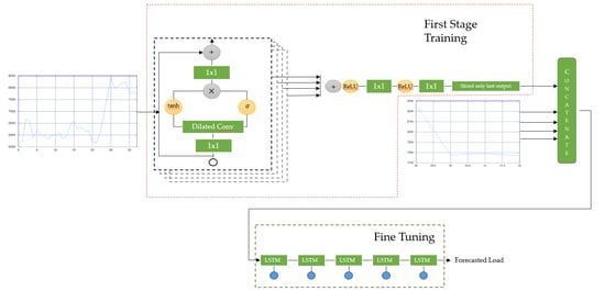
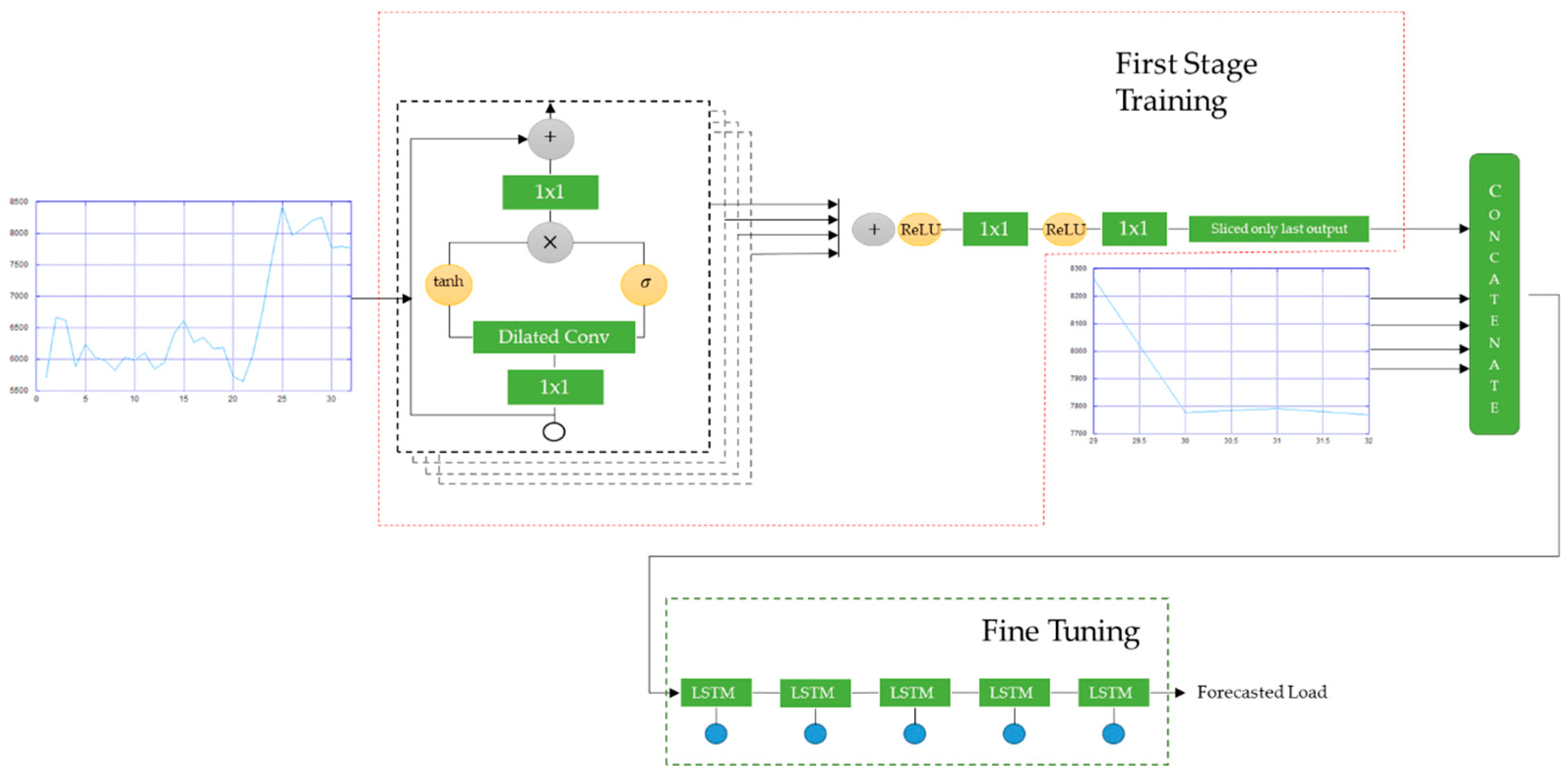
Complete representation of our model is depicted in Figure 8. The wavenet-based model is fed by 32 data sequences containing information of load demand and time index information (clock, day, and month). This wavenet model is used for the initial forecasting algorithm based on long sequence data. Before fed to dilated CNN, long sequence data are prepossessed using standard 1D-CNN with filter size equal to one. Next, the prepossessed data is convoluted by dilated causal CNN with filter size of 2. All of the convolutional layers have ReLU activation function expressed as:

$$f\left(x\right)=\max \left(0,x\right)$$

(14)

In the case of the residual network, the total residual block in our model is 10 with a dilation rate set to be a repetition of a sequence dr = [1, 2, 4, 8, 16]. Dilation rate is a hyperparameter that represents how large the gap between the element of the filter is, as shown in Figure 4 and indicated by the arrows. All of the residual blocks are summed followed by the ReLU activation function. The post-processing is conducted before the last convolutional layer which works similar with time distributed fully connected layer in which it is assigned for normalization of the residual output.

Because the length of input and output in the dilated causal CNN are identical, then the customize layer is built for taking only the last output’s neuron representing load at t = 33. After completing the wavenet-based network training, the output of the last convolutional layer is concatenated with recent data sequences (t = 29 until t = 32) that work as LSTM input. Here, by using the fine tuning technique, LSTM with linear activation function is assigned to make self-correction of convolutional output in order to provide more accurate prediction based on short sequence. This self-correction method is nearly identical to how humans make a prediction based on data sequences. For example, in predicting the environment temperature, humans will relate the understanding between the temperature trend from the previous day with the recent temperature trend in order to make an accurate prediction for the next hour temperature.

Table 1. Forecasting result obtained using dataset 1.

Layer	Parameters
Input Layer (1)	32, 44
Conv1D (1)	[f, ks, s] = [16, 1, 1]
Dilated Causal Conv1D	[f, ks, s, dr] = [32, 2, 1, dr]
Conv1D (2)	[f, ks, s] = [16, 1, 1]
Conv1D (3)	[f, ks, s] = [128, 1, 1]
Conv1D (4)	[f, ks, s] = [1, 1, 1]
Input Layer (2)	5, 1
LSTM	1 output node

shows the summary of our model’s parameter where f, ks, s, and dr are the number of filters, kernel size, stride, and dilation rate, respectively. Loss function and optimizer are mean absolute error and adaptive and momentum (ADAM) [26], respectively, and batch size is 512. The model was trained using Nvidia GTX 1070, Tensorflow 1.13.1 [27], CUDA 10, and CuDNN 7.6.2 with 500 epochs and the final model is chosen based on the validation accuracy.

4. Result and Discussion

4.1. Model Performance Evaluation

In order to evaluate our model performance, we mainly compared this model with the two previous deep learning-based models that work very well in the case of STLF. Those models are inspired by [15] (Model 1), which utilizes stacked LSTM and [16] (Model 2) which combines the stacked CNN and LSTM layer with the feature fusion layer. The configuration of each comparison model is identical to the published papers. Model 1 consists of two stacked LSTM layers consisting of 20 units followed by fully connected layers as an output layer. Model 2 is built with a combination between the LSTM and CNN layer where their outputs are concatenated, which is eventually fed to the fully connected layer called a feature fusion layer. All of the models are trained with the same input data. Moreover, the original wavenet model is also used for a model comparison in order to prove the benefit of LSTM as a self-correction layer in our proposed model.

This section reports on the performance of hourly load forecasting by using our proposed method compared to other forecasting methods. In the testing stage, all of the models are evaluated with three difference commonly used metrics, root mean squared error (RMSE), mean absolute error (MAE), and mean absolute percentage error (MAPE). MAE is the average of absolute difference values between predicted load and actual load consumption. MAPE is just identical to MAP but it uses a ratio between the difference with the actual load while RMSE is another metric that tends to have a higher value compared to other metrics. The higher value which results from the metrics, the worse performance of the model. Those metrics are defined as follow:

$$\mathrm{RMSE}= \sqrt{\frac{1}{N}{\displaystyle \sum }_{i=1}^N{\left(\widehat{y_i}-y_i\right)}^2}$$

(15)

$$\mathrm{MAE}= \frac{1}{N}{\displaystyle \sum }_{i=1}^N\left|\widehat{{\widehat{y}}_i}-y_i\right|$$

(16)

$$\mathrm{MAPE}= \frac{1}{N}{\displaystyle \sum }_{i=1}^N\left|\frac{\widehat{{\widehat{y}}_i}-y_i}{y_i}\right|$$

(17)

4.2. ENTSO-E Load Prediction

Table 2. Forecasting result obtained using European Network of Transmission System Operators for Electricity (ENTSO-E) testing dataset 1.

Model	RMSE	MAE	MAPE (%)
Tian et al.	240.57	171.71	2.45
Kong et al.	222.44	155.83	2.22
Wavenet	217.98	157.28	2.24
Our Model	203.23	142.23	2.02

and

Table 3. Forecasting result obtained European Network of Transmission System Operators for Electricity (ENTSO-E) testing dataset 2.

Model	RMSE	MAE	MAPE (%)
Tian et al.	306.77	216.19	3.42
Kong et al.	304.07	209.22	3.29
Wavenet	305.04	212.99	3.36
Our Model	292.07	196.95	3.1

show all of the models’ performance on dataset 1 and dataset 2, respectively. Overall, our proposed model outperforms other models, especially in the case of dataset 1 where the data distribution is nearly identical with the validation data, while the worst performance is shown by [16]-based model. In Table 2, our proposed model clearly shows its excellence over other methods which shows the success of the combination between deep residual causal CNN and LSTM using fine tuning technique in understanding long sequence and short sequence data, respectively. Moreover, compared to the standard wavenet model, our model performs better accuracy indicating the usefulness of the LSTM layer in making self-correction for initial load forecasting output by dilated causal residual CNN.

However, all of models exhibit downgraded performance in dataset 2. It indicates that all of the model still cannot understand data which has slightly different distribution with training, validation, and testing data 1. The failure of all of the models in testing using dataset 2 is highly affected by the quality of the ENTSO-E dataset where the inconsistency of hourly power usage or unpredicted trends occur several times. Figure 9 and Figure 10 show the result of STLF on dataset 1 and dataset 2, respectively.

4.3. ISO-NE Load Prediction

Table 4. Forecasting result obtained using Independent System Operator New England (ISO-NE) testing dataset 1.

Model	RMSE	MAE	MAPE (%)
Tian et al.	114.33	82.18	0.56
Kong et al.	92.7	62.55	0.42
Wavenet	109.76	77.69	0.52
Our Model	85.12	58.96	0.4

and

Table 5. Forecasting result obtained using Independent System Operator New England (ISO-NE) testing dataset 2.

Model	RMSE	MAE	MAPE (%)
Tian et al.	141.97	89.07	0.66
Kong et al.	100.5	65.12	0.48
Wavenet	125.11	78.02	0.57
Our Model	88.31	62.23	0.46

show all of models performance on ISO-NE dataset 1 and dataset 2 respectively. Different with performances shown in the previous subsection, all of the models perform very well both in known and unknown data distribution. However, the model based on [16] still exhibits the worst accuracy, while our model still performs the best although its excellence is not absolute compared to the model based on [15]. Same with the result obtained using the ENTSO-E dataset, the implementation of the LSTM layer for tuning the wavenet-based model, is proven to help the network in making more accurate load predictions.

The success of all models in understanding an unknown data distribution in this dataset is mainly because of the ISO-NE data property, which is simpler compared to the ENTSO-E dataset in which more fluctuations are experienced in certain ranges of time due to external factors. This simplicity results in high accuracy both in validation and testing data, enabling all models to handle forthcoming data sequences. Figure 11 and Figure 12 show the forecasting result using input from dataset 1 and dataset 2, respectively.

4.4. Discussion

Overall, our proposed model shows the best performance compared to the other deep learning-based models. It indicates that each network in the proposed model works very well. The wavenet-based network provides understanding of long sequence data and the LSTM layer helps the model do self-correction by relating the output of the first network with the recent or short sequence data.

However, as suggested by [12,28,29], in order to show our proposed model significance over the other models, both the Wilcoxon signed rank test [30] and Friedman test [31] are conducted using all the models’ forecasting error given input from those testing datasets. The Wilcoxon signed rank test will compare the $W_{statistic}$ with the Wilcoxon critical value $W$ which are expressed in Equations (18) and (19) (for huge number of data), respectively.

$$W_{statistic}= \min \left\{r^{+},r^{-}\right\}$$

(18)

$$W= \frac{N\left(N+1\right)}{4}$$

(19)

$r^{+}$ and $r^{-}$ are the sum of the positive and negative rank, respectively, while $N$ is the number of data. If $W_{statistic}$ is less than $W$, and the p-value is less than α, then the null hypothesis is rejected, and it indicates the superiority of our model.

On the other hand, the Friedman test is applied to show the significant differences of our proposed models over all comparison models. The statistic F is expressed by:

$$F= \frac{12N}{k\left(k+1\right)}\left[{\displaystyle \sum }_{j=1}^k{R}_j{}^2-\frac{k{\left(k+1\right)}^2}{4}\right]$$

(20)

where $N$ is the number of forecasting results, $k$ is the number of compared models, and $R_j$ is the average rank sum based on forecasting error $r$ for $j$th compared model expressed by:

$$R_j= \frac{1}{N}{\displaystyle \sum }_1^N{r}_i{}^j$$

(21)

If the p-value of F is less than the critical value, than the null hypothesis is not accepted, indicating the superiority of our model.

Table 6. Result of the Wilcoxon signed-rank test and Friedman test using ENTSO-E testing dataset 1.

Compared Models	Wilcoxson Signed-Rank Test				Friedman Test
	α = 0.025 W = 285,423	p-value	α = 0.05 W = 285,423	p-value	α = 0.05
Our Model vs Kong et al.	243,792	3.64 × 10−5	243,792	3.64 × 10−5	$H_0:e_1=e_2=e_3=e_4$ F = 47.4618 p = 2.77 × 10−10 (Reject $H_0$)
Our Model vs Tian et al.	211,190.5	1.81 × 10−13	211,190.5	1.81 × 10−13
Our Model vs Wavenet	246,095	9.60 × 10−5	246,095	9.60 × 10−5

,

Table 7. Result of the Wilcoxon signed-rank test and Friedman test using ENTSO-E testing dataset 2.

Compared Models	Wilcoxson Signed-Rank Test				Friedman Test
	α = 0.025 W = 80,792	p-value	α = 0.05 W = 80,792	p-value	α = 0.05
Our Model vs Kong et al.	68,149.5	0.001227	68,149.5	0.001227	$H_0:e_1=e_2=e_3=e_4$ F = 17.59 p = 0.00053 (Reject $H_0$)
Our Model vs Tian et al.	66,885	3.77 × 10−4	66,885	3.77 × 10−4
Our Model vs Wavenet	69,587	0.004169	69,587	0.004169

,

Table 8. Result of the Wilcoxon signed-rank test and Friedman test using ISO-NE testing dataset 1.

Compared Models	Wilcoxson Signed-Rank Test				Friedman Test
	α = 0.025 W = 285,423	p-value	α = 0.05 W = 285,423	p-value	α = 0.05
Our Model vs Kong et al.	274,482	2.78 × 10−1	274,482	2.78 × 10−1	$H_0:e_1=e_2=e_3=e_4$ F = 140.032 p = 3.72 × 10−30(Reject $H_0$)
Our Model vs Tian et al.	179,311	6.68 × 10−26	179,311	6.68 × 10−26
Our Model vs Wavenet	206,826.5	6.43 × 10−15	206,826.5	6.43 × 10−15

and

Table 9. Result of the Wilcoxon signed-rank test and Friedman test using ISO-NE testing dataset 2.

Compared Models	Wilcoxson Signed-Rank Test				Friedman Test
	α = 0.025 W = 80,792	p-value	α = 0.05 W = 80,792	p-value	α = 0.05
Our Model vs Kong et al.	80,556	0.950686	80,556	0.950686	$H_0:e_1=e_2=e_3=e_4$ F = 40.198 p = 9.67 × 10−9 (Reject $H_0$)
Our Model vs Tian et al.	57,955	5.29 × 10−9	57,955	5.29 × 10−9
Our Model vs Wavenet	66,618.5	0.00029	66,618.5	0.00029

show the significance test in testing dataset 1 and dataset 2 ENTSO-E and testing dataset 1 and 2 ISO-NE, respectively. In the Wilcoxon signed-rank test, significant levels are set to α = 0.025 and α = 0.05 while in the Friedman test it is conducted only under α = 0.05. From results showed in the tables, our proposed model shows significant contribution in forecasting accuracy improvement and superiority over the other models, except in the ISO-NE dataset, where in the Wilcoxon signed rank test between our proposed model and Kong et al. model the results indicate no significance, although the results in terms of RMSE, MAE, and MAPE show that our model performs better.

5. Conclusions and Future Works

This paper proposes a novel method for hourly load forecasting case which is very important in the case of demand response for hybrid energy systems, especially for system use of both renewable and fossil energy in order to reduce fossil energy usage. The proposed method is mainly inspired by the wavenet-based model utilizing dilated causal residual CNN and LSTM. In this approach, two different data sequences are fed to the model. The long data sequences are fed to the wavenet-based model while the short data sequences are fed to the LSTM layer assigned for model self-correction using fine-tuning technique.

In order to prove the generality of our model, two different datasets, which are the ENTSO-E and ISO-NE dataset, are used with two different testing scenarios. The first testing scheme uses the dataset having nearly identical distribution with the validation dataset, while the second uses a dataset from slightly different data distribution. Based on the obtained result, our proposed model exhibits the best performance compared to other deep learning-based models in terms of RMSE, MAE, and MAPE. In detail, our model achieves RMSE, MAE, and MAPE equal to 203.23, 142.23, and 2.02 for ENTSO-E testing dataset 1 and 292.07, 196.95, and 3.1 for ENTSO-E dataset 2. Meanwhile, in the ISO-NE dataset, the RMSE, MAE, and MAPE equal to 85.12, 58.96, and 0.4 for ISO-NE testing dataset 1 and 85.31, 62.23, and 0.46 for ISO-NE dataset 2. However, there are several findings that can be improved in future work. The first is in the ENTSO-E dataset testing result; all models cannot provide high accuracy forecasting if they are fed using slightly different data distribution. It indicates that all models face difficulties in understanding fluctuated or unpredicted data like the ENTSO-E dataset. The second is although RMSE, MAE, and MAPE show our model exhibits better accuracy compared to the Kong et al. model in the ISO-NE dataset, our model cannot provide a significant improvement.

Therefore, for future work, additional external factors data like information of holidays and weather conditions can be fed as the models’ input in order to improve our findings. In addition, building a new model can also be conducted since this research area and artificial intelligence (AI) algorithms are developed very quickly, making a new idea come up very fast. All of the codes and datasets used in this research are available on Github.

References

1. Krishna, K.S.; Kumar, K.S. A review on hybrid renewable energy systems. Renew. Sustain. Energy Rev. 2015, 52, 907–916. [Google Scholar] [CrossRef]
2. Olson, C.; Lenzmann, F. The social and economic consequences of the fossil fuel supply chain. MRS Energy Sustain. 2016, 3. [Google Scholar] [CrossRef] [Green Version]
3. Siano, P. Demand response and smart grids—A survey. Renew. Sustain. Energy Rev. 2014, 30, 461–478. [Google Scholar] [CrossRef]
4. Nguyen, D. Demand Response for Domestic and Small Business Consumers: A New Challenge. In Proceedings of the IEEE PES T&D 2010, New Orleans, LA, USA, 19–22 April 2010; pp. 1–7. [Google Scholar]
5. Marwan, M.; Kamel, F.; Xiang, W. Mitigation of electricity price/demand using demand side response smart grid model. In Proceedings of the 1st International Postgraduate Conference on Engineering, Designing and Developing the Built Environment for Sustainable Wellbeing (eddBE 2011), Brisbane, Australia, 27–29 April 2011; Queensland University of Technology: Brisbane, Australia, 2011; pp. 128–132. [Google Scholar]
6. Vu, D.H.; Muttaqi, K.M.; Agalgaonkar, A. A variance inflation factor and backward elimination based robust regression model for forecasting monthly electricity demand using climatic variables. Appl. Energy 2015, 140, 385–394. [Google Scholar] [CrossRef] [Green Version]
7. Al-Hamadi, H.; Soliman, S. Short-term electric load forecasting based on Kalman filtering algorithm with moving window weather and load model. Electr. Power Syst. Res. 2004, 68, 47–59. [Google Scholar] [CrossRef]
8. Cho, M.; Hwang, J.; Chen, C. Customer Short Term Load Forecasting by Using ARIMA Transfer Function Model. In Proceedings of the 1995 International Conference on Energy Management and Power Delivery EMPD’95, Singapore, 21–23 November 1995; pp. 317–322. [Google Scholar]
9. Hao, C. A new method of load forecasting based on generalized autoregressive conditional heteroscedasticity model. Autom. Electr. Power Syst. 2007, 15, 12–13. [Google Scholar]
10. Niu, D.; Wang, Y.; Wu, D.D. Power load forecasting using support vector machine and ant colony optimization. Expert Syst. Appl. 2010, 37, 2531–2539. [Google Scholar] [CrossRef]
11. Fan, G.-F.; Guo, Y.-H.; Zheng, J.-M.; Hong, W.-C. Application of the Weighted K-Nearest Neighbor Algorithm for Short-Term Load Forecasting. Energies 2019, 12, 916. [Google Scholar] [CrossRef]
12. Dong, Y.; Zhang, Z.; Hong, W.-C. A hybrid seasonal mechanism with a chaotic cuckoo search algorithm with a support vector regression model for electric load forecasting. Energies 2018, 11, 1009. [Google Scholar] [CrossRef]
13. Zhang, R.; Dong, Z.Y.; Xu, Y.; Meng, K.; Wong, K.P. Short-term load forecasting of Australian National Electricity Market by an ensemble model of extreme learning machine. IET Gener. Transm. Distrib. 2013, 7, 391–397. [Google Scholar] [CrossRef]
14. Ghofrani, M.; Ghayekhloo, M.; Arabali, A.; Ghayekhloo, A. A hybrid short-term load forecasting with a new input selection framework. Energy 2015, 81, 777–786. [Google Scholar] [CrossRef]
15. Kong, W.; Dong, Z.Y.; Jia, Y.; Hill, D.J.; Xu, Y.; Zhang, Y. Short-term residential load forecasting based on LSTM recurrent neural network. IEEE Trans. Smart Grid 2017, 10, 841–851. [Google Scholar] [CrossRef]
16. Tian, C.; Ma, J.; Zhang, C.; Zhan, P. A Deep Neural Network Model for Short-Term Load Forecast Based on Long Short-Term Memory Network and Convolutional Neural Network. Energies 2018, 11, 3493. [Google Scholar] [CrossRef]
17. Han, L.; Peng, Y.; Li, Y.; Yong, B.; Zhou, Q.; Shu, L. Enhanced deep networks for short-term and medium-term load forecasting. IEEE Access 2018, 7, 4045–4055. [Google Scholar] [CrossRef]
18. Park, K.; Yoon, S.; Hwang, E. Hybrid load forecasting for mixed-use complex based on the characteristic load decomposition by pilot signals. IEEE Access 2019, 7, 12297–12306. [Google Scholar] [CrossRef]
19. LeCun, Y.; Bengio, Y. Convolutional networks for images, speech, and time series. Handb. Brain Theory Neural Netw. 1995, 3361, 1995. [Google Scholar]
20. Hochreiter, S.; Schmidhuber, J. Long short-term memory. Neural Comput. 1997, 9, 1735–1780. [Google Scholar] [CrossRef]
21. Oord, A.V.D.; Dieleman, S.; Zen, H.; Simonyan, K.; Vinyals, O.; Graves, A.; Kalchbrenner, N.; Senior, A.; Kavukcuoglu, K. Wavenet: A generative model for raw audio. arXiv 2016, arXiv:1609.03499. [Google Scholar]
22. He, K.; Zhang, X.; Ren, S.; Sun, J. Deep residual learning for image recognition. In Proceedings of the IEEE Conference on Computer Vision and Pattern Recognition, Las Vegas, NV, USA, 26 June–1 July 2016; pp. 770–778. [Google Scholar]
23. Handbook-Glossary, U.O. European network of transmission system operators for electricity. Available online: https://transparency.entsoe.eu/load-domain/r2/totalLoadR2/show (accessed on 30 April 2019).
24. Shamsollahi, P.; Cheung, K.; Chen, Q.; Germain, E.H. A neural network based very short term load forecaster for the interim ISO New England electricity market system. In Proceedings of the PICA 2001. Innovative Computing for Power-Electric Energy Meets the Market. 22nd IEEE Power Engineering Society. International Conference on Power Industry Computer Applications (Cat. No. 01CH37195), Sydney, Australia, 20–24 May 2001; pp. 217–222. [Google Scholar]
25. Goodfellow, I.; Bengio, Y.; Courville, A. Deep Learning; MIT Press: Cambridge, MA, USA, 2016. [Google Scholar]
26. Kingma, D.P.; Ba, J. Adam: A method for stochastic optimization. arXiv 2014, arXiv:1412.6980. [Google Scholar]
27. Abadi, M.; Barham, P.; Chen, J.; Chen, Z.; Davis, A.; Dean, J.; Devin, M.; Ghemawat, S.; Irving, G.; Isard, M. Tensorflow: A system for large-scale machine learning. In Proceedings of the 12th {USENIX} Symposium on Operating Systems Design and Implementation ({OSDI} 16), Savannah, GA, USA, 2–4 November 2016; pp. 265–283. [Google Scholar]
28. Diebold, F.X.; Mariano, R.S. Comparing predictive accuracy. J. Bus. Econ. Stat. 2002, 20, 134–144. [Google Scholar] [CrossRef]
29. Derrac, J.; García, S.; Molina, D.; Herrera, F. A practical tutorial on the use of nonparametric statistical tests as a methodology for comparing evolutionary and swarm intelligence algorithms. Swarm Evolut. Comput. 2011, 1, 3–18. [Google Scholar] [CrossRef]
30. Wilcoxon, F. Individual comparisons by ranking methods. In Breakthroughs in Statistics; Springer: New York, NY, USA, 1992; pp. 196–202. [Google Scholar]
31. Friedman, M. A comparison of alternative tests of significance for the problem of m rankings. Ann. Math. Stat. 1940, 11, 86–92. [Google Scholar] [CrossRef]
Figure 1. Average daily power consumption of each dataset.
Energies 12 03359 g001
Figure 2. Example of one-day load demand of each dataset (a) ISO-NE dataset; (b) ENTSO-E dataset.
Energies 12 03359 g002
Figure 3. Load demand trend over a year.
Energies 12 03359 g003
Figure 4. Dilated causal convolutional neural network with filter size 2.
Energies 12 03359 g004
Figure 5. Residual learning process.
Energies 12 03359 g005
Figure 6. Overview of residual dilated convolutional block and gated activation function.
Energies 12 03359 g006
Figure 7. Comparison between simple recurrent neural network (RNN) and long short-term memory (LSTM) layer: (a) simple RNN layer, (b) LSTM layer.
Energies 12 03359 g007
Figure 8. Proposed model architecture.
Energies 12 03359 g008
Figure 9. Forecasting result using ENTSO-E dataset 1.
Energies 12 03359 g009
Figure 10. Forecasting result using ENTSO-E dataset 2.
Energies 12 03359 g010
Figure 11. Forecasting result using ISO-NE dataset 1.
Energies 12 03359 g011
Figure 12. Forecasting result using ISO-NE dataset 2.
Energies 12 03359 g012