A Novel Direct Load Control Testbed for Smart Appliances

Abstract

The effort to continuously improve and innovate smart appliances (SA) energy management requires an experimental research and development environment which integrates widely differing tools and resources seamlessly. To this end, this paper proposes a novel Direct Load Control (DLC) testbed, aiming to conveniently support the research community, as well as analyzing and comparing their designs in a laboratory environment. Based on the LabVIEW computing platform, this original testbed enables access to knowledge of major components such as online weather forecasting information, distributed energy resources (e.g., energy storage, solar photovoltaic), dynamic electricity tariff from utilities and demand response (DR) providers together with different mathematical optimization features given by General Algebraic Modelling System (GAMS). This intercommunication is possible thanks to the different applications programming interfaces (API) incorporated into the system and to intermediate agents specially developed for this case. Different basic case studies have been presented to envision the possibilities of this system in the future and more complex scenarios, to actively support the DLC strategies. These measures will offer enough flexibility to minimize the impact on user comfort combined with support for multiple DR programs. Thus, given the successful results, this platform can lead to a solution towards more efficient use of energy in the residential environment.

1. Introduction

Much has been written about the new role consumers can play in future smart grid (SG). Driven by the massive integration of renewable energy resources, the SG is evolving swiftly, causing changes in how electricity is produced, managed, marketed, and consumed. If for a while, the SG paradigm meant merely accepting a bi-directional flow of electricity and information, it must continue to evolve to adapt to the current demands of the digital consumer. In the years to come, the computational exploitation of the enormous amounts of information provided by the Internet of Things (IoT) sensors, incorporated at all layers of the SG, will become the main engine of its evolution towards the digital energy network, focused on customer service. This is what has been called “data-driven energy” [1]. A large amount of energy data will support collective decision making, opening the way to more responsive utilities and more engaged consumers. This will undoubtedly impact the evolution of household appliances. In fact, SAs are already showing their potential for data-driven energy [2].

The growing use of energy by domestic appliances shows no signs of slowing, reaching 2900 TWh in 2017. The use of electricity by these loads continues to grow by almost 2% per year, a steady trend since 2010 [3]. Although the electricity demand for major appliances has slightly decreased since 2007, mainly due to improvements in their energy efficiency, the rapid proliferation of small appliances and brown goods has absorbed these savings. The energy consumption due to these small loads has grown twice as fast as that of large appliances in the last decade. In addition, only one-third of domestic appliances consumption is under regulatory protection, particularly in emerging markets. This may become even more relevant in the near future as the demand for electricity in buildings increases due to the impact of the charging infrastructure for electric vehicles. While it is true that there is a need to increase the rigor of existing policies by extending regulatory coverage to a broader range of devices, on the other hand, user awareness may be the key factor. However, to achieve this, consumers should be rewarded to some extent when changing their behavior. The availability of information and communication technologies (ICT) on SG can be decisive in meeting this commitment through the widespread adoption of DR strategies.

In other areas, such as power electronics, it is common to find a complete chain of modeling, development, testing, optimization, virtual validation, and rapid prototyping commercial tools that integrate seamlessly into a convenient testing and development environment such as these tools of Typhoon (Typhon, Somerville, USA) [4] and dSPACE (dSPACE, Paderborn, Germany) [5]. It is possible to find testbed proposals for different applications in SG, like our previous one [6]. In the newly released paper [7], a distributed framework for real-time management and co-simulation of DR in SG is presented. This solution provides a near real-time co-simulation platform to validate new DR-policies exploiting IoT approach performing software-in-the-loop. In the recent papers, authors propose an interesting testbed for distributed DR based on a microgrid (MG) modeled on the PSIM software (Powersim, Rockville, USA) to provide frequency regulation [8] and control over other grid parameters in general [9]. In the model, the nodes of virtual IoT devices are created according to the collective characteristics of their real twins, connected to the system. Network conditions can be reproduced when testing new DR algorithms to provide, e.g., frequency regulation reserve services.

Similarly, in order to support the field of DLC research in this emerging application area of SA, it is necessary to provide new testbeds for lab experimentation. Therefore, the main contribution of this work is the development of a research test bench flexible enough to incorporate different tools of different origins such as weather forecasting APIs, DR providers from the utility and mathematical optimization features built on the basis of the LabVIEW systems (2015, National Instruments, Austin, USA) design platform and development environment for a visual programming language. It can benefit from user-friendly and intuitive software as well as hardware such as powerful real-time processors, user-programmable field-programmable gate array (FPGA), and full I/O interfaces. However, although it also offers libraries of dedicated functions, it has been necessary to specifically develop a sophisticated software (that did not exist) that supports the seamless link between the tools, since their individual parts are precisely aligned with each other. In this sense, the proposed testbed is a novelty since most of the papers available in the literature are focused on the development of complex mathematical models without considering the integration of these tools that are so important to implement a realistic platform and thus emulate scenarios and test cases as real as possible. Furthermore, this work is a step forward from previous research, as it includes several tools that have never been integrated before.

The organization of the paper as follows. Section 2 and Section 3 presents the background of the research. Then, Section 4 describes the experimental platform and also examines the control and optimization strategies, considering practical limitations and safety constraints in detail. In Section 5, the case study is discussed. Finally, the conclusions and future work are reported in Section 6.

2. Home Energy Management Systems (HEMS) State of the Art

The combination of the SG paradigm with IoT technologies and the will of consumers to actively participate in their energy control has enhanced the HEMS concept. These are systems capable of monitoring home consumption at different levels and implementing automation or control mechanisms.

They have evolved at an unstoppable pace in the last years. By 2013, most systems only offered home monitoring, either local or remote and rarely some manual control over switches or dimmable loads [10].Currently, on the contrary, a wide variety of control systems are available ranging from the simple automatic scheduling of applications to the optimization of energy resources, through advanced algorithms that consider the state of numerous external variables such as energy prices or weather conditions. What is more, they are even able to learn from users thanks to the incorporation of artificial intelligence [11].

Because of this evolution and the large range of devices and algorithms that are being integrated into the HEMS, the number of works in the literature is extensive and unapproachable for a paper whose purpose is not that. However, for example, the authors in [12] define a classification according to the level of complexity of these systems. This will help to situate the present work and the challenges addressed. The levels from the lowest to the highest complexity are Monitoring, Logging, Alarm, Energy Management, and DR.

Nowadays, the first three levels can be regarded as a prerequisite. Every HEMS must carry out home monitoring at different aggregation levels. The basic level is the total household consumption, generally measured by technologies such as Smart Meters, widely deployed across Europe [13]. Nevertheless, the energy footprint of individual elements can be recorded by means of load submetering or non-intrusive load monitoring (NILM) algorithms, which use machine learning to distinguish individual appliances from the total consumption [14].

The capture of measures can be performed with different granularity and be stored in different supports. In this way, all or part of the data is stored in the cloud, from where it is possible to obtain descriptors or apply machine learning algorithms. This also allows for the possibility of generating alarms at different levels, so fast events that require immediate attention can be generated and then processed in the so-called Edge, while more complex alarm mechanisms can be implemented in higher layers after preprocessing and analysis of historical data.

The aforementioned elements are essential for the creation of reliable controls at the next levels named: energy management and DR. The first focuses on the control of a combination of distributed resources to guarantee a continuous power supply, whereas the second goes a step further and manages the individual consumer appliances.

Among the recent publications, the most used optimization techniques are mixed-integer linear-programming [15], and variation of those [16], as well as population-based algorithms [17]. It is also common to find works that propose multi-objective algorithms to reach a trade-off between the energy savings that can be achieved and the benefits from possible incentives [18].

Nevertheless, as is evident from the most recent publications, the use of Internet technologies as a solution to optimization problems is becoming more and more common [19], as they tackle issues such as the diversity of household appliances, the simultaneous pursuit of several objectives in parallel, and the uncertainty in predicting conditions such as occupancy levels, energy consumption or weather conditions [20].

3. Smart Appliances Overview

What is a SA? There is more than one definition, but popularly a SA is recognized because it has some degree of embedded processing and wireless connectivity. Sometimes called a Net appliance, an Internet appliance or an information appliance, it can be as simple as an application that warns you whenever your refrigerator has a door opened, or as complex as remotely controlling your oven from your smartphone or via a voice assistant. However, in the framework of the SG, the term “smart” focuses on those systems (with communications-enabled) which are able to modulate their electricity consumption in response to external signals such as price information [21], local measurements [22] or direct control commands [23]. In other words, those appliances that can support grid flexibility because they have been configured to respond to DR requests.

In a recent survey [24], 28% of people find SA very attractive, but people are more reluctant to buy them because of price concerns, so 49% of people say this is a barrier to buying. Other barriers include dynamic pricing, lack of interoperability and legal framework as reported by the European parliament [25] and the world economic forum [26]. First, the lack of a dynamic pricing model to the clear majority of customers is an obstacle. Users will not be willing to change their habits if they cannot perceive that this intelligent functionality can bring them substantial financial savings. Second, the high purchase premiums and long replacement cycles of these devices are prolonging their mass adoption. Thirdly, to enable the communication between SAs that use different protocols and standards, and to ensure interoperability, the communication interface must be supported by a data model that conforms to a harmonized reference ontology. A semantic platform called OpenFridge has recently been proposed in [27] that has been deployed and evaluated with real-life users distributed globally. But the candidate for such a reference ontology will almost certainly be the Smart Appliances REFerence ontology (SAREF) [28]. SAREF4ENER [29] is the SAREF extension to be able to fully support DR for the energy domain.

Finally, the lack of a clear legal structure around customer data limits growth in this area. This could include the appliance energy use pattern meaning when, how much and how is energy being consumed. These data could even be monetized. For example, appliance manufacturers might be willing to pay an energy supplier a fee for these data, as they can be of great value in terms of customer service, product support, as well as maintenance. In the case of aggregation [30], how this data could be shared among customers to allow, e.g., for their energy efficiency comparison. An aggregator can operate on behalf of a group of consumers, having access to data and possible remote adjustment over consumers’ appliances. If the security of connected devices used in aggregation is not safeguarded, consumers could be exposed to several risks like data theft or request of appliance ransomware. Security flaws and data privacy issues are main concerns of the users, and only a few regions have well-defined rules about who can access, own, and share utility customer data.

However, the prospects for SA are bright. The global market for SA is projected to reach $38.35 billion by 2020, with a compound annual growth rate (CAGR) of 16.6% over the projected period 2015–2020. IoT-enabled devices (currently low, about 5% of white goods) are expected to grow dramatically, and the number of sensors is expected to increase six-fold by 2020. So, according to the International Energy Agency, by 2040 almost 1 billion households and 11 billion SA could participate in interconnected electricity systems.

Typically, DR policies can be classified between load-shifting strategies, which move the load from on-peak or event hours when demand and rates are the highest, to off-peak hours when rates are lower, and load-shedding strategies, which directly reduce or avoid energy use during on-peak hours altogether. Consequently, in the residential sector, the loads can be divided into non-shiftable, time-shiftable and energy “sheddable”. The time-shiftable loads are the appliances whose operation can be moved from peak to off-peak times with the minimal loss of comfort for the inhabitant. This is the category of ‘wet’ appliances, e.g., dishwashers (DW), washing machines (WM), and tumble dryers (TD). These appliances account for a significant proportion of household energy consumption. Alternatively, non-shiftable loads, such as lighting and brown appliances, cannot delay their operation [31]. At present, there is no deployed infrastructure that allows remote activation of these appliances. However, their behavior has been deeply studied and it is now possible to understand the potential of the DR in supporting the operation of the network [32].

Among household appliances, a special category is the thermostatically-controlled loads (TCL) (e.g., electric water heaters (EWH), HVAC systems, refrigerators, and freezers) as their thermal inertia allows for flexible load patterns (both shifting and shedding) while meeting their service requirement. Therefore, compared to other SA, TCL exhibit predictable behavior from the DR point of view, and even more when aggregated in large population clusters [33]. In recent work, a stochastic model has been presented for the generation of high temporal resolution synthetic profiles of the consumption of these domestic appliances [34]. However, its potential for flexibility remains virtually unknown. [35] presents the recent projects that are facilitating the transition from research to development. In general terms, and due to their inherent characteristics, there are two types of TCL, with different operating principles. First, resistive loads (i.e., heat generation equipment) and, second, compressor-driven loads (i.e., heat pumping equipment). Although this paper is particularly dealing with resistive loads, greater demand elasticities could be achieved if the control strategy achieved were extended to the rest of the residential TCL.

4. Structure of the Smart Appliance Control Testbed

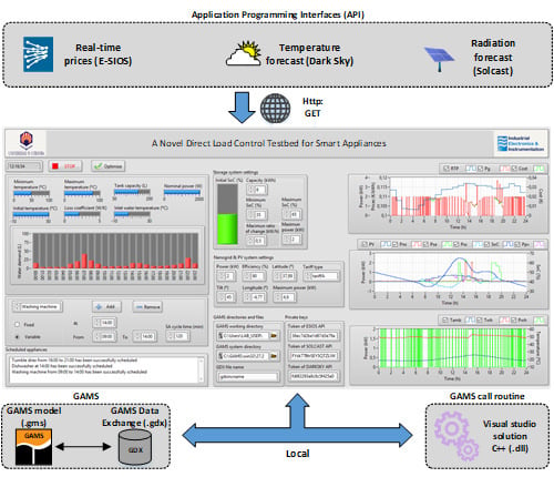
The proposed control platform is composed of four main blocks that collect data and exchange information between each other aiming to implement the abovementioned DR policies through DLC. The platform architecture is shown in Figure 1, where LabVIEW works as the core application by handling the data provided by the outer blocks. This central block also has the highest priority from the call handling point of view, that is, LabVIEW follows the classical scheme where the main application deals with the so-called subVI to allow modular designs. At the same time, this subVIs will be the interfaces with the rest of the blocks.

The block on the right side is related to the API that provides the testbed with both weather information (Ambient temperature and photovoltaic (PV) production forecast) and the price of the energy.

Finally, these DR policies must be mathematically translated into an optimization model which includes several constraints related to the people’s habits, the availability of energy from different sources and the household appliances features among others. The model should also offer a certain degree of flexibility with respect to the number of invokes and formulation changes. All these reasons have contributed to opt for General Algebraic Modelling System (GAMS) as the software used to solve the proposed model. Furthermore, another component including the functions given by the GAMS API is used to integrate this software into LabVIEW using a dynamic link library (DLL). The following sections will describe these previous blocks and their interactions in more detail.

4.1. LabVIEW

LabVIEW has been the tool used to integrate and manage all blocks of the platform. Concretely, the developed LabVIEW application consists of two threads commonly known as while loops located in the block diagram. The first one implements the whole infrastructure necessary to parametrize and call the GAMS model and comprises the data collection from the API solcast [36], dark sky [37] and Spanish system operator information system (E-SIOS) [38], which is the information system of the Spanish electricity group Red Eléctrica de España (REE), using the subVI getAPIData.vi that implements an hypertext transfer protocol (HTTP) client. This loop also entails the data standardization with respect to the sampling times by means of dataConv.vi, the model call through callDLL.vi as will be described in the following section and the display of the results. However, the second loop just converts the raw information of the scheduled SA (name, operation mode, and time) into a recognizable information by the model through getSAData.vi.

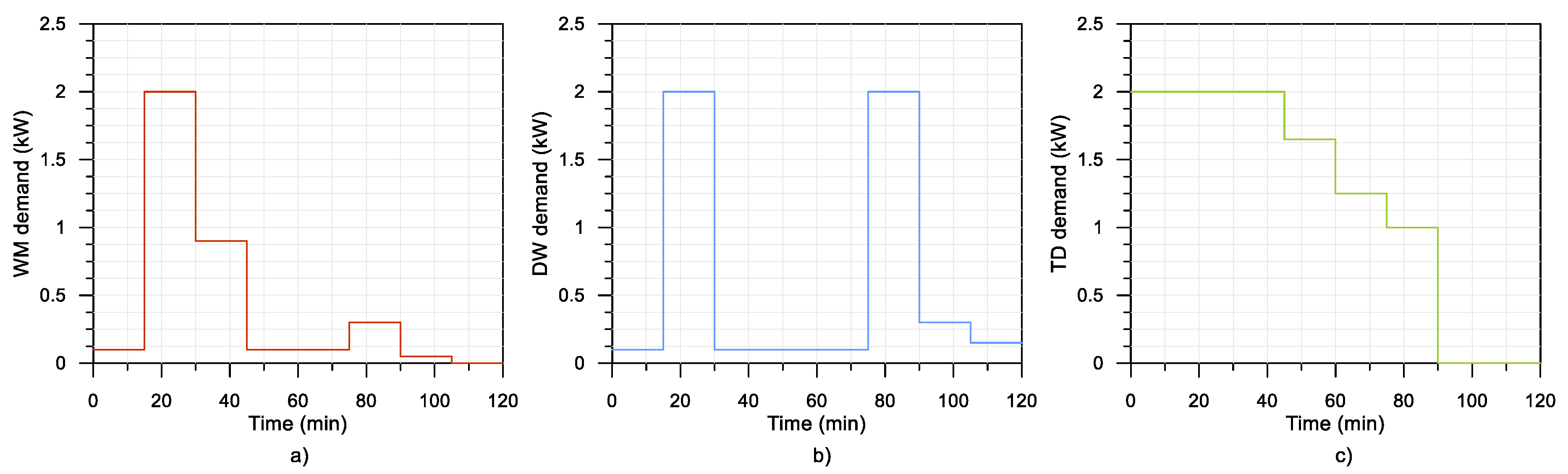
The graphic user interface (GUI) or front panel is shown in Figure 2 and has three main parts, namely, the SA scheduler (part A) including at the top the EWH section where the parameters that model this appliance (Minimum and maximum temperatures, tank capacity, nominal power, initial temperature, loss factor, inlet water temperature, and the hourly hot water consumption) are set up. The rest of SA under analysis in this study (WM, DW, and TD) are modeled according to their average power consumption and are scheduled at the bottom of part A where both the time and mode of operation as well as the cycle time can be selected. Two modes of operations have been evaluated: The fixed mode is used to launch the SA at a fixed time while the variable mode enables a certain degree of flexibility since the SA is scheduled over a time interval. As a result, the platform is forced to decide the start time within this interval once the model is solved. This part also includes information (Name, operation mode and time) about the scheduled SA.

At the top of the part B are the parameters that model the energy storage system (ESS) such as the initial state of charge (SoC), capacity, minimum, and maximum SoC allowed as well as maximum power flow and a maximum ratio of change. At the middle, some features of the nanogrid under study can be found: Geographical coordinates (Longitude and latitude), tilt angle, power and efficiency in the case of the PV system or maximum power and tariff type with respect to the grid connection. The last section in part B includes the local directories required by GAMS, on the left half, and the personal keys that API administrator provides to establish a secure connection, on the right half.

Finally, part C shows the results of the optimization process divided into three graphs. From top to bottom, the first graph plots the hourly price of the energy according to the selected tariff, the optimal power consumption from the grid and thus the cost once these two previous ones are known. The second graph shows profiles such as the SoC and power taken from the batteries, the PV production and the amount of such power that would be injected into the nanogrid, the power usage of the SA and the consumption to be considered non-shiftable. The last graph describes the whole state of the EWH depicting its power consumption as well as the water and ambient temperatures.

4.2. Linking GAMS and LabVIEW

This section describes the communication between GAMS and LabVIEW. Some papers show the integration of GAMS into Matlab [39] or other software like LabVIEW through Matlab as an intermediary interface [40]. In this sense, the novelty of this work is the direct coupling of both tools without using any intermediate software. On the one hand, the inner communication between the GAMS model and its GAMS Data Exchange (GDX) file has been included under the subsection GAMS as appears in Figure 1. 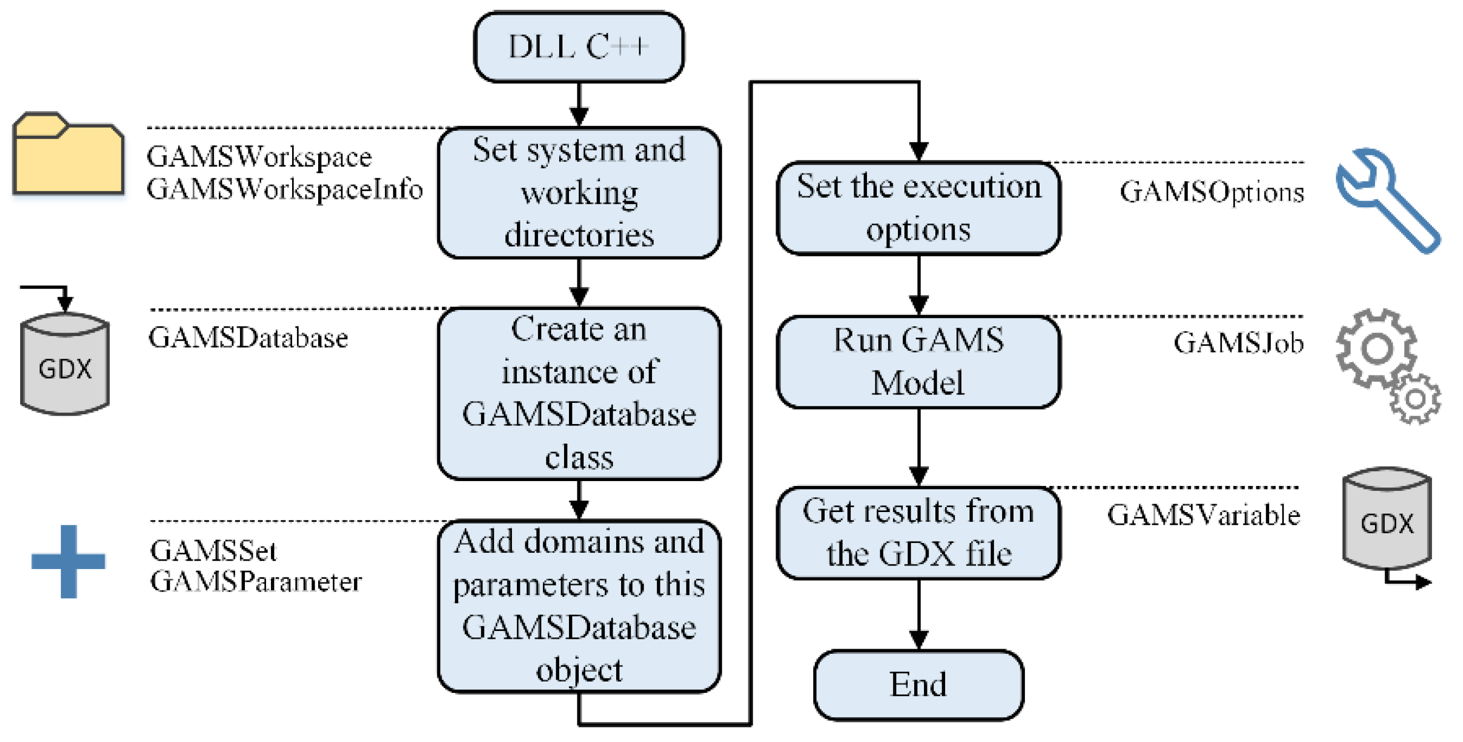This file is often used to store the parameters with which the model is called, as well as the model results, however, such interaction does not take place directly but will have to be handled by means of the appropriated classes and methods that the GAMS object-oriented API [41] provides resulting in the seamless integration of GAMS into any application such as LabVIEW in this case. This architecture employs the C++ API in a DLL format which is the interface that makes the linkage possible. The flowchart is shown in Figure 3. First, system and working directories have been set; the system directory refers the path where all GAMS installation files are located while the working directory refers to the path where the GAMS models and GDX files will be stored (also shown in part B of Figure 2). The second stage aims to create a database object where the parameters used in the model will be stored, but this will be carried out in the third stage. The model execution options, such as the names of the database object and the exchange file to be used are subsequently specified. The last stages are in charge of executing the model, returning the optimal values of the decision variables.

4.3. An Optimization Model for Demand-Side Management

While most of the proposed models address this issue as a task scheduling problem using heuristics algorithm to make decisions on shifting, shedding or even disconnecting the load, this paper proposes a novel mixed-integer linear programming (MILP) model that uses the price-based DR programs to optimize the power consumption using the potential flexibility that TCL provides to the demand. The proposed model involves a smart home with its own ESS, distributed energy resources (DER) based on PV panels as well as a scenario with SA managed through the DLC strategy.

In terms of mathematical formulation, Equation (1) refers to the objective function $f$ (in $€$) where $P_g\left(t\right)$ (in kW, as all the powers henceforth) and $Pr\left(t\right)$ (in €/kWh) are the power consumption from the grid and the price of the energy respectively at time slot $t\in \left[1,2,\dots T\right]$. The rest of the equations are constraints related to the power balance, the user preferences and the energy availability from the sources. Equation (2) denotes the global power balance at each time slot $t$ with $P_g\left(t\right)$, the power taken from the PV panels $P_{pv}\left(t\right)$ as well as the power given by the energy storage system $P_{ess}\left(t\right)$ on the generation side. On the demand side is the non-shiftable power $P_{ns}\left(t\right)$, which involves the stand-by consumption coming from non-dimmable devices, such as lighting, low power DC adapters used to supply small devices and also the consumption from the SA scheduled in fixed mode, $P_s\left(t\right)$ is the power consumption of the common-use SA such as the WM, DW and TD scheduled in variable mode and the consumption of the EWH expressed as the product of its nominal power $P_{wh}$ and the binary variable $x_{wh}\left(t\right)$ that indicates its state each time slot.

Equations (3)–(5) set the limits for $P_g\left(t\right)$, $P_{pv}\left(t\right)$ and $P_{ess}\left(t\right)$ respectively, where $P_g^{max}$ denotes the maximum power that can be taken from the grid and $P_{ess}^{max}$ the maximum power that can be injected into or extracted from the ESS. Moreover, the ratio of change of this variable has also been constrained in Equation (8) through the parameter $d{P}_{ess}^{max}$ (in kW/h) in order to ensure a lifetime of the batteries as long as possible. Finally, $f_{pv}\left(P_{pv}^{pk},{\eta }_{pv},\alpha ,\lambda ,\varphi ,t\right)$ refers to the function that implements solcast to provide the PV production each time slot $t$ and thus has been taken as the maximum power available to be injected into the system from the PV panels. Parameters such as the installed peak power $P_{pv}^{pk}$, the efficiency ${\eta }_{pv}$, the tilt angle $\alpha$ or the location, through the latitude $\lambda$ and longitude $\varphi$ will be required by this API in each HTTP request.

Equations (6) and (7) describe the dynamic of the ESS by means of a simple kWh counter to compute the current state of charge $SoC\left(t\right)$ (in %) based on the previous one $SoC\left(t-1\right)$ and $P_{ess}\left(t\right)$ and setting the $SoC\left(t\right)$ limits between $So{C}_{min}$ and $So{C}_{max}$ not to allow deep charges and discharges which is also a condition to ensure a long lifetime of the system.

The SA scheduling process using the variable mode is modeled by Equations (9) and (10) and has been conceived as a decision-maker who chooses the optimal SA operation from among the possible ones that could be generated between the selected start and end times, by shifting the original consumption one-time slot. In this context, let us define $j$ as the index that refers to each SA to be scheduled and $k_j$ the index associated with each shifted consumption that may be generated for each $j$, being $N_j$ the number of SA and $N_k^j$ the number of possible consumption profiles. This family of shifted consumptions builds each matrix ${\Gamma }_j\left(k_j,t\right)$ which has as many rows as possible scenarios and as many columns as considered time slots $T$. Moreover, for the decision-making process, all the shifted consumptions have been associated with a binary variable $x_j\left(k_j\right)$ and thus, the optimal scenario will be indicated once the model is solved by means of the state of these decision variables. Finally, to ensure just one shifted consumption operates, Equation (9) forces the sum so that just one binary variable is equal to 1.

The EWH has been considered as a special SA due to its thermal inertia and therefore has its own power balance equation as it is apparent from (11). From left to right, this balance involves the energy stored inside the EWH tank characterized by the current and previous average water temperature $T_{wh}\left(t\right)$ and $T_{wh}\left(t-1\right)$ (in °C, as the rest of temperatures hereafter), the tank capacity $C_{wh}$ (in m³) and the parameters that model essential features of the supply water like its density $\rho$ (in kg/m³) and its specific heat $C_p$ (in kJ/kg·°C). The following terms are the thermal losses taking place in the tank walls given by the loss factor $g_{wh}$ (in kW/°C) and the ambient temperature profile $T_{amb}\left(t\right)$ besides the energy provided by the water entering the tank as a consequence of the usage events and defined by means of the hot water consumption $D_{wh}\left(t\right)$ (in m³/s) and the temperature of this water, $T_{inlet}$. Finally, the discrete energy due to the heater element can be found. Once the EWH dynamic has been well-defined, the model for this appliance is fully completed with Equation (12) where the upper and lower limit of $T_{wh}\left(t\right)$ are constrained according to the normal operation temperatures $T_{wh}^{min}$ and $T_{wh}^{max}$.

$$Min f=\frac{24}{T}{\displaystyle \sum }_{t=1}^T{P}_g\left(t\right)Pr\left(t\right)$$

(1)

S.t:

$$P_g\left(t\right)+P_{pv}\left(t\right)+P_{ess}\left(t\right)=P_{ns}\left(t\right)+P_s\left(t\right)+x_{wh}\left(t\right)P_{nwh}$$

(2)

$$0\le P_g\left(t\right)\le P_g^{max}$$

(3)

$$0\le P_{pv}\left(t\right)\le f_{pv}\left(P_{pv}^{pk},{\eta }_{pv},\lambda ,\varphi ,t\right)$$

(4)

$$-P_{ess}^{max}\le P_{ess}\left(t\right)\le P_{ess}^{max}$$

(5)

$$SoC\left(t\right)=SoC\left(t-1\right)-100\left(\frac{24}{T}\right)\frac{P_{ess}\left(t\right)}{C_{ess}}$$

(6)

$$So{C}^{min}\le SoC\left(t\right)\le So{C}^{max}$$

(7)

$$-d{P}_{ess}^{max}\le \frac{P_{ess}\left(t\right)-P_{ess}\left(t-1\right)}{\raisebox{1ex}{$24$}\!\left/ \!\raisebox{-1ex}{$T$}\right.}\le d{P}_{ess}^{max}$$

(8)

$$P_s\left(t\right)={\displaystyle \sum }_{j=1}^{N_j}{\displaystyle \sum }_{k_j=1}^{N_k^j}{x}_j\left(k_j\right){\Gamma }_j\left(k_j,t\right)$$

(9)

$${\displaystyle \sum }_{k_j=1}^{N_k^j}{x}_j\left(k_j\right)=1$$

(10)

$$\begin{gathered} C_{wh}\rho C_p\frac{T_{wh}\left(t\right)-T_{wh}\left(t-1\right)}{\raisebox{1ex}{$86400$}\!\left/ \!\raisebox{-1ex}{$T$}\right.}=g_{wh}\left[T_{amb}\left(t\right)-T_{wh}\left(t-1\right)\right] \\ +D_{wh}\left(t\right)\rho C_p\left[T_{inlet}-T_{wh}\left(t-1\right)\right]+x_{wh}\left(t\right)P_{nwh} \end{gathered}$$

(11)

$$T_{wh}^{min}\le T_{wh}\left(t\right)\le T_{wh}^{max}$$

(12)

5. Case Study

This section aims to evidence the effectiveness of the above-described DLC platform by testing it under cases which consist of minimizing the cost of the energy imported from the grid over a 24-h time horizon, as was stated in the previous section, with a time resolution of 5 min, so that, $T=288$. Concretely, two case studies based on the available electricity tariffs in the Spanish market are considered. One case is based on time discrimination in two periods (off-peak and peak) also known as tariff DHA, and another is a case using the default tariff or tariff A (without time discrimination).

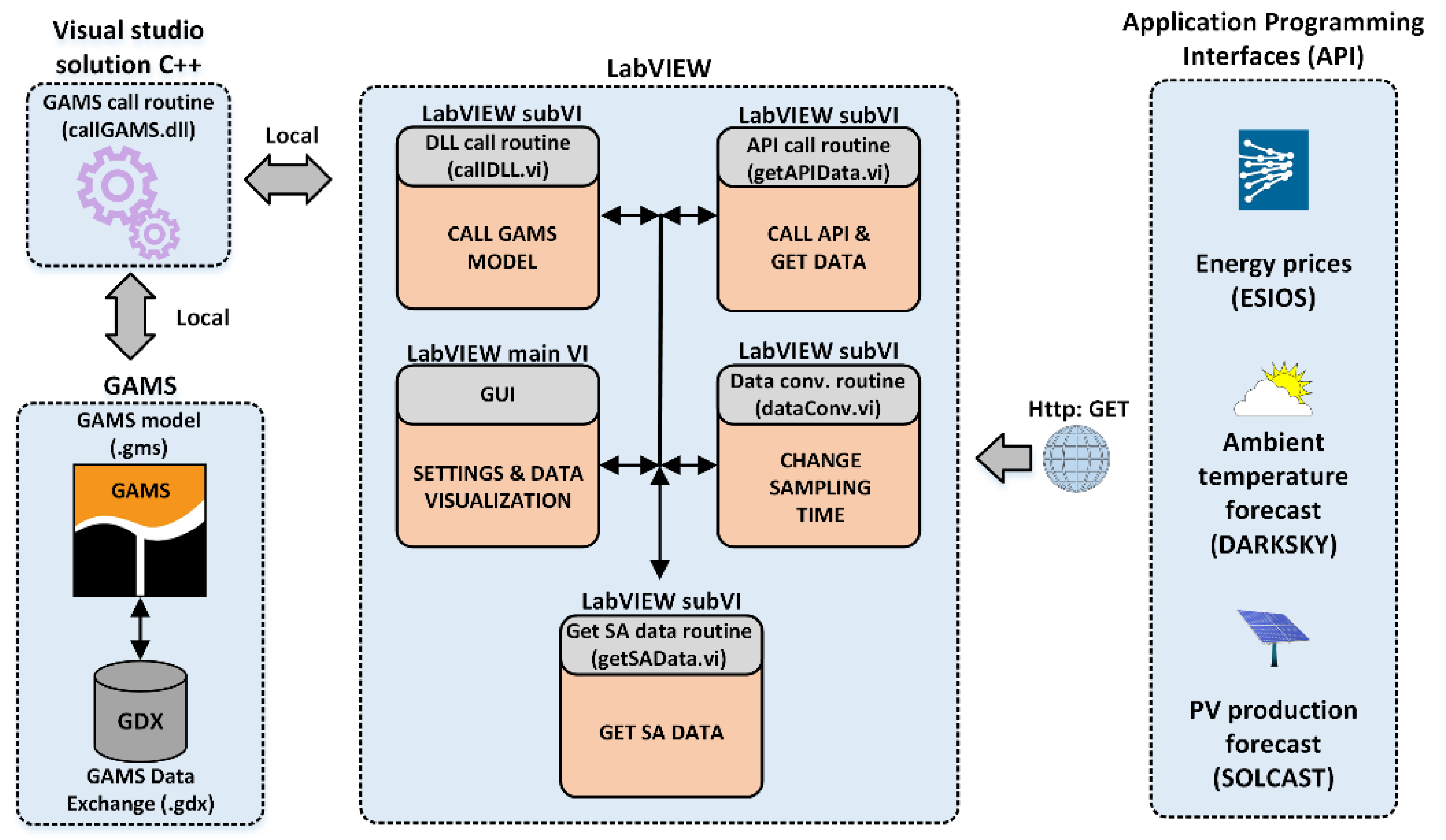
Both cases use the SA consumption models shown in Figure 4 and based on 120 min working cycle divided into 8 slots of 15 min provided by [42].

Additionally, to give the case study a more realistic approach, the component of the non-shiftable power that represents the standby consumption was obtained by acquiring the active power in one of the laboratory circuits for a 24-h workday.

Under this framework, a typical dwelling including a small scale ESS and PV installation has been chosen as the topology of this case study. More in detail, the PV system is modeled by a nominal power of 2 kW, an efficiency of 90% and mounted with a tilt angle of 30°. With respect to the location, southern Spain has been considered for both cases, concretely at 37.88° and −4.79° of latitude and longitude respectively. On the other hand, the ESS has a capacity of 6 kWh, a maximum charge/discharge power of 2 kW with a ratio of change limited to 0.5 kW/h and where the SoC can fluctuate in the range 35–65%, the initial SoC was fixed to 50%. The EWH considered is the type which can be found in the residential environment, vertically mounted and cylindrical, with a capacity of 0.1 m³ as well as a nominal power of 2 kW. Its loss factor has been set to 2·10⁻³ kW/°C and the inlet water temperature to 21 °C [43], while the water temperature inside the tank has been constrained in the range 60–85 °C with an initial condition of 65 °C. In addition, an example of hot water consumption considering the water drawn from the EWH tank due to household use such as hand washing, showering, and dishwashing among others and based on [44] has been used. Finally, the capacity of the main grid has been fixed to 4.6 kW since it is a common value in Spain.

Table 1. Main parameters of the model.

Subsystem	Parameter	Value	Subsystem	Parameter	Value
Main grid	$P_g^{max}$	4.6 kW	EWH	$C_{wh}$	0.1 m3
ESS	$P_{ess}^{max}$	2 kW		$g_{wh}$	2·10−3 kW/°C
	$C_{ess}$	6 kWh		$T_{inlet}$	21 °C
	$d{P}_{ess}^{max}$	0.5 kW/h		$T_{wh}^{min}$	60 °C
	$So{C}^{min}$	35%		$T_{wh}^{max}$	85 °C
	$So{C}^{max}$	65%		$T_{wh}\left(0\right)$	65 °C
	$SoC\left(0\right)$	50%		$P_{nwh}$	2 kW
PV	$P_{pv}^{pk}$	2 kW		$C_p$	4.18 kJ/kg·°C
	${\eta }_{pv}$	90%		$\rho$	988 kg/m3
	$\alpha$	30°
	$\lambda$	37.88°
	$\varphi$	−4.79°

summarizes the main parameters of the model as well as its values.

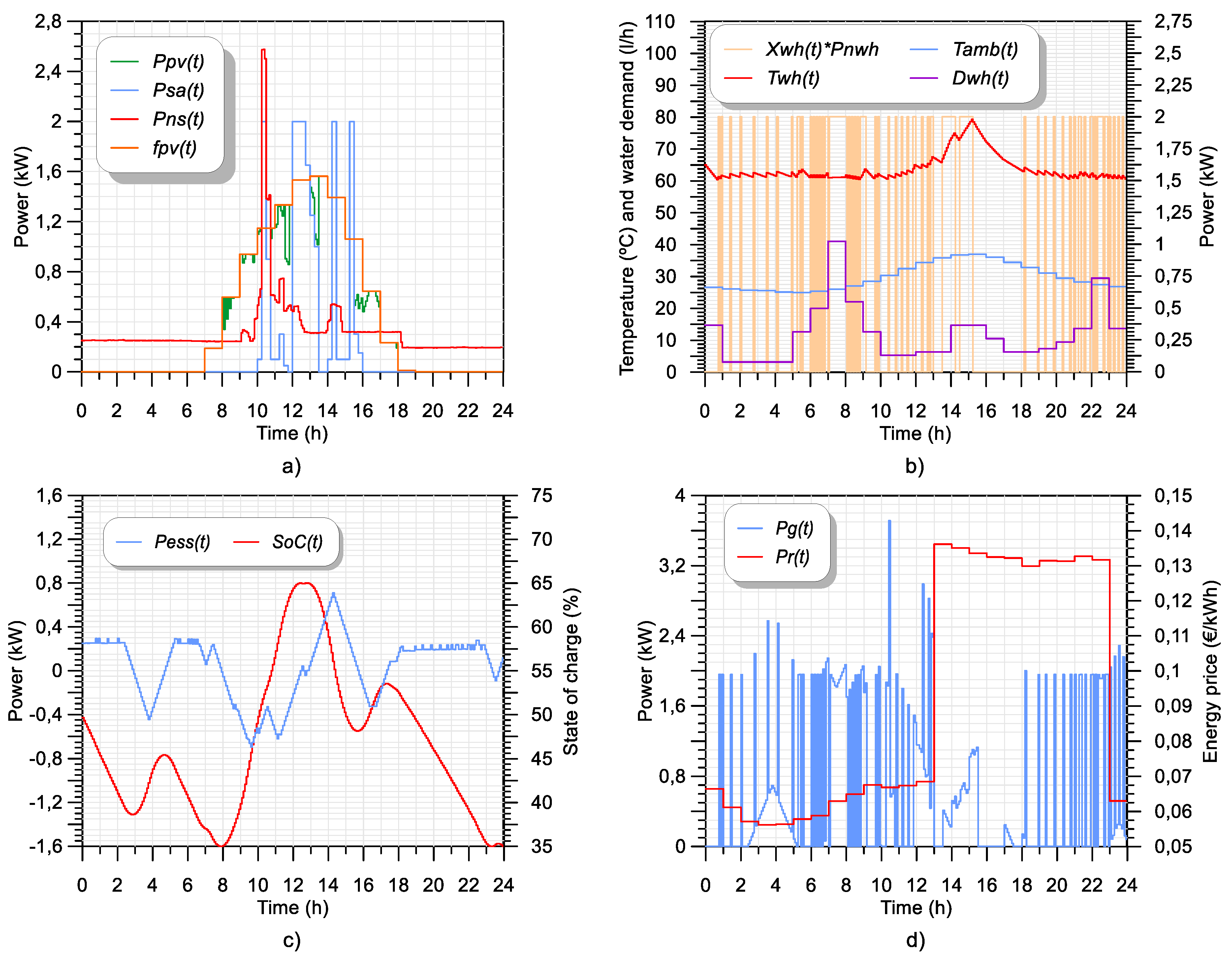
Figure 5 introduces the first case in which tariff A with both scheduling mode (variable and fixed) have been used, depicting a 24-h horizon. Particularly, in this case, the scheduling configuration for the SA has been set as follows: Washing machine scheduled from 09:00 to 14:00, tumble dryer scheduled from 16:00 to 21:00 and dishwasher fixed at 14:00.

Note from Figure 5a the result of the scheduling process and the times at which the SA start their operation cycles. As it is apparent from $P_{sa}\left(t\right)$, which is the decoupled consumption of all the SA scheduled in either fixed or variable mode, the washing machine starts almost at midday (at 11:45), around the peak of the prices although a large amount of this demand is covered by the PV system. The dishwasher at 14:00 (as was stated) and tumble drier is shifted until 18:00 where the second valley of the price can be found. This behavior shows a clear strategy of searching for the lowest price or the highest PV production to launch these SA. In view of the results, all the initial constraints related to the scheduling period are clearly satisfied.

The non-shiftable consumption is denoted by the red line of the same figure including the fixed consumption of the dishwasher at 14:00 and the experimentally measured example in which the period of highest activity falls in the range 09:00–18:00 according to the laboratory timetables. The green line shows the power injected into the system from the PV panels, which represents 9.78 kWh, and has not the same value that the PV production shown in orange (10.65 kWh) and provided by solcast. In this case, the system does not use all the energy to achieve the most economical way, however, the amount of this one taken from the main grid is greater than if the PV energy were fully employed.

Figure 5b depicts the EWH behavior using the above-mentioned hot water demand (expressed in L/h instead of m³/s for easier comprehension) and the hourly temperature profile provided by dark sky (see purple and blue lines respectively). The EWH consumption shown in orange evolves in the range 0–2 kW due to it’s on/off operation. Before 12:00, the water temperature is more or less constant and the power consumption behaves in agreement to the water consumption so that a water demand variation causes a proportional energy consumption, which means this energy is mainly used to warm the inlet water. In fact, the highest energy consumption in this interval takes place at the peak of water demand. On the contrary, at midday, the water consumption is not significative and thus, this energy is intended to increase the water temperature inside the tank from 60 °C to 83 °C, considering multiple favorable conditions such as the greater availability of energy coming from the PV system, the high ambient temperature as well as the amount of charge already stored in the ESS. This temperature increment enables to face the future water drawn acts, which is a desirable strategy in response to DR events as it is the presence of high market prices in this interval. Later, the temperature slowly falls up to 60 °C at 20:00 due to the water consumption and remains constant the rest of the day.

The ESS shows a clear policy based on the energy price (red line in Figure 5d) and PV production. The initial SoC was set to 50% and quickly decreases to supply the non-shiftable power until 02:00 reaching almost 39% in a high-priced environment. Afterward, the off-peak of the prices can be found and $P_{ess}\left(t\right)$ go up as fast as possible (due to the slope of $P_{ess}\left(t\right)$ matches to $d{P}_{ess}^{max}$) to retrieve some charge previously lost, which is equivalent to shift the amount of energy that belongs to $P_{ns}\left(t\right)$, from the beginning of the day to the off-peak interval. During this interval $P_{ns}\left(t\right)$ is supplied by means of the main grid. At 04:30 the SoC drops again to repeat the same process with $P_{ns}\left(t\right)$ and reaches the minimum value allowed (35%) at 08:00. Once here, the PV system begins to inject power that goes directly to the ESS resulting in a charging process that carries the SoC from 35% to 65% to address the SA consumption with the help of $P_{pv}\left(t\right)$ during the most expensive interval (12:00–15:00). The rest of time follows the same principle as explained above: Charge process in presence of the second off-peak of the price (15:00–17:30) and subsequent discharge to supply both the tumble drier and the non-shiftable power (17:30–00:00). The total energy exported and imported by the system was 3.89 and 3.00 kWh respectively. Another important detail is the effect of $d{P}_{ess}^{max}$ over $P_g\left(t\right)$: Previous tests were done with a more relaxed value prove that a larger amount of the EWH energy can be absorbed by ESS as this would enable better tracking of demands with higher ratios of change. Finally, in Figure 5d the hourly prices and the main grid consumption can be found. The foregoing description of this case is also reflected in $P_g\left(t\right)$ and makes it possible the main objective of avoiding and capitalizing the peak and off-peak of $Pr\left(t\right)$ respectively. The daily price for this case was 1.80 € with a total demand of energy that almost achieves 16.10 kWh.

For the following case, the configuration for the SA has been set as follows: Washing machine fixed at 10:00, tumble dryer scheduled from 12:00 to 20:00 and dishwasher scheduled from 14:00 to 19:00.

Figure 6a (blue line) shows how the model has decided to launch the dishwasher and tumble drier at the lower limit of the scheduling period which allows the system benefits from the PV production (depicted in orange and kept constant from the previous case) and the ESS that also supplies part of this consumption, especially after 13:00, where the prices are much higher than in the previous half. The washing machine operates at 10:00 as expected. The PV production is not fully intended to be injected into the system (just 9.96 of 10.65 kWh) as is evidenced by $P_{pv}\left(t\right)$, in green, and which also took place in the case above. With respect to the non-shiftable demand, the previous part corresponding to the stand-by consumption has been used, including the demand of the washing machine at 10:00.

Both the ESS and EWH have similar behaviors with respect to the previous case but with some exceptions. Figure 6b shows the performance of the EWH under the same assumptions as of the first case (water demand, ambient temperature, water temperature limits, and initial conditions) although the temperature increment begins one hour earlier and is more progressive. Furthermore, the temperature rises at one of the peaks of the water demand while the water was warmed up before this maximum in the first case. The ESS also performs similar, which evidences the PV production has a higher weight in its behavior than the energy price. Moreover, with respect to $Pr\left(t\right)$, it is more important the shape of the function, concretely the maxima and minima location, than the absolute values. The energy exported and imported in this case reaches 3.45 and 2.55 kWh. Finally, Figure 6d introduces the prices, that splits the day in two well-defined half, and the consumption from the main grid where the most consumption is located in the cheapest region as desired and entails an amount of 15.75 kWh (11.8 kWh from 23:00 to 13:00 compared to 3.95 kWh the rest of time). The daily price was 1.30 €.

Once these previous cases have been presented,

Table 2. Result summary.

	ESS		PV		Main Grid
Case	Imported Energy (kWh)	Exported Energy (kWh)	Injected Energy (kWh)	Energy Production (kWh)	Energy Imported (kWh)	Objective Function: Price (€)
Case 1: Tariff A	3.00	3.89	9.78	10.65	16.10	1.80
Case 2: Tariff DHA	2.55	3.45	9.96	10.65	15.75	1.30

summarizes the results. Obviously, case 2 achieves a better performance with respect to the objective function and thus, tariff DHA enables to more efficient utilization of elements such as DER and ESS in presence of thermal loads that contribute to the flexibility of the system as in this case the EWH.

6. Conclusions and Future Work

In the current context of increasing energy use in the residential environment, where most consumption comes from the SA use, the employment of DR policies is essential to deal with this type of loads through a DLC paradigm with the goal of reaching higher efficient management of the energy resources. This paper has proposed an original architecture that supports research and development, and integrates tools that are very diverse and complementary aiming to develop a platform that brings together the best features of all of them, such as the high mathematical performance of GAMS, the accuracy of the weather forecasting applications as well as the flexibility of LabVIEW as the linking tool. Later both cases studies have been carried out to prove the high capabilities of the testbed with successful results, placing the adopted solution as an attractive alternative towards a higher energy performance dwelling ambient.

Finally, as future work, the authors leave the real-time control of the DER, ESS, and loads in the primary and secondary control of a real MG. In this context, the developed platform would perform as a day-ahead demand scheduler in the tertiary control although additional communication channels would need to be deployed to enable the interface with the lower hierarchical level. Furthermore, the mathematical model written in GAMS and thus the developed DLL would also have to be adapted to the MG needs, however, due to the reconfigurable nature of the system, this would not take more than a few minutes. Hence, this platform could be migrated to be used in a real microgrid expecting the same performance, but these considerations must be considered.