A Stochastic Model for Residential User Activity Simulation

Abstract

User activities is an important input to energy modelling, simulation and performance studies of residential buildings. However, it is often difficult to obtain detailed data on user activities and related energy consumption data. This paper presents a stochastic model based on Markov chain to simulate user activities of the households with one or more family members, and formalizes the simulation processes under different conditions. A data generator is implemented to create fine-grained activity sequences that require only a small sample of time-use survey data as a seed. This paper evaluates the data generator by comparing the generated synthetic data with real data, and comparing other related work. The results show the effectiveness of the proposed modelling approach and the efficiency of generating realistic residential user activities.

1. Introduction

In the field of civil engineering, energy modelling and simulation of buildings need to take into account the activities of users in order to achieve better accuracy [1]. The energy efficiency of a building depends not only on the structure of the building itself, but also on the behaviour of its occupants. Once a dwelling has been occupied, the energy consumption only varies according to the activities of the occupants. This can be understood from the evidence that similar households in similar buildings can have significant differences in energy consumption, and that the change of household inhabitants can lead to significant changes in energy consumption. With the use of new technologies and services in the residential sector, it is possible to study the impact of the dynamic changes of user activities on energy consumption accurately. Energy consumption depends, among other things, on the activity patterns of residents, while these patterns can vary to hours of the day and the day of the week [2]. Therefore, user activity patterns can be used as one of the inputs for the load modelling for individual households, and for the whole residential sector. Utilities can also accurately predict energy demand and provision energy. However, due to the lack of dynamic activity data from residents, it is difficult to combine user activity profiles with energy prediction.

In addition, it is necessary to synthesise user activity data for privacy reasons. Today, many countries, including the Scandinavian countries, Denmark and Sweden, restrict the dissemination and use of personal data by law. The recent enforcement of the EU Regulation on General Data Protection (GDPR) [3] requires strong privacy protection for personal data. This makes it difficult to publish data related to personal privacy, such as data on user activities. Therefore, simulation is a viable way to provide user activity data.

In this paper, we present a stochastic model for the simulation of residential user activities for single- and multi-family households. This model is based on a Markov chain, which was developed on specific Time Use Survey (TUS) data Danish data in this study). The Markov chain model comprises eight possible states, including sleeping, cooking, dishwashing, laundry, cleaning, leisure, away from home and others. Based on the model, we develop a data generator to generate user activity sequences. Although the model is developed based on Danish TUS data, it can easily be extrapolated to the other TUS data, due to the generic nature of the model. The generated activity profiles can be made available to the public in open data platforms and used e.g., for estimating the electricity consumption of the appliance of interest [4].

Definition 1 (Time-use survey).

A time use survey is a statistical survey that aims to report how people spend their time. It is used to identify, classify and quantify the main types of activities that people engage in during a definitive time period, such as a day, a week, a month or a year [5].

The contributions of this paper are summarized as follows: (1) We develop a Markov chain stochastic model for simulating residential user activities; (2) we formalize the model, and the method to generate activity data for different types of households; (3) we implement the model training program using an in-database machine learning method, and implement a parallel data generator using a multi-threading method; and (4) we evaluate the model comprehensively, compare related work and validate its effectiveness and efficiency in generating a large user activity data set.

The remainder of this paper is organized as follows. Section 2 gives a review of related work. Section 3 describes the problem and overview. Section 4 presents the modelling method of user activities. Section 5 describes the implementation of a user activity sequence generator. Section 6 evaluates the activity model and the data generator. Section 7 concludes the paper and points to future research directions.

2. Related Work

A number of research efforts were found on energy modelling incorporating user activities, mainly in the energy and building sectors. In the early work [6], a bottom-up approach was introduced to model the impact of user activities on demand-side management for residential households. According to individual activity patterns, Muratori et al. modelled the electricity demand of multi-family households [7]. Widen et al. [8,9] related residential electricity demand to occupancy profiles based on time-use survey data. Richardson et al. created a domestic electricity demand model based on UK’s TUS data [10], which can generate one-minute granular data for individuals, households, or neighbourhoods. Eoghan et al. investigated activity-based demand models suitable for demand-response simulations [11]. Many other works translate household routines into energy loading profiles, in combination with appliance parameters, including [8,10,12,13,14,15]. These works, however, focus on the application of user activities or behaviours in demand-side energy consumption modelling et al. and convert activities (based on time-use survey data) into energy consumption for an individual or a household. This also stresses the importance of incorporating user behaviour data to modelling tasks in order to obtain better results. These works, however, haven’t explained how to model user activities. Our work, instead, focuses on residential activity modelling, and its aim is to provide activity data to energy modelling tasks without breaking user privacy. As our model uses TUS data, we expect that the resulting activity data can be used for modelling energy load profiles accurately.

Various occupancy models have been found in the literature, and all these models were established based on using TUS data, some together with other support data sets, such as household information. The most common approach is the use of the Markov chain to model residential activities, including [8,10,16,17], as well as the approach presented in this paper. However, they differ in the number of states and the supplement approaches used. The works [16,17] focus on the three most basic occupancy states, including sleep, active and absent. Richardson et al. identify active occupancy profile of users by calculating the probability of the occurrence of an activity [10]. The model is calibrated using date types, occupants and households. Palacio et al. models human activities into work and not work, and links occupancy to energy usage [1]. However, their approach is for modelling the activities of the people who work in the industrial sector. In addition to the probability models, Aksanli et al. develop a graph-based model to represent the chain of user activities [18], and Basu et al. use a decision tree in their modelling [19].

Table 1. The approaches of activity Modelling using Time Use Survey (TUS) data.

Ref.	Data	Data Size	Resolution	Modelling Method	Modelling Purpose
[10,16]	UK TUS	1000	10 min	Markov chain (3 states)	Occupancy and energy
[8]	Swedish TUS	431 persons in 103 detached houses and 66 apartments	Down to 1 min	Markov chain (9 states)	Load profiles
[17]	Belgian TUS, Household budget survey	3455 households	10 min	Markov chain (3 states)	Occupancy
[1]	Harmonised European TUS	19295 people from 9541 households.	10 min	Markov chain (2 states)	Occupancy
[18]	American TUS, Energy consumption survey	10000+ participants	10min	Directed graph	Activities and electricity usage of appliance
[19]	IRISE database [20]	900 households	24/48/168 h	Decision tree	Electricity usage of appliance

summarises the reviewed literature that use TUS data for activity modelling. Note that this is not a comprehensive survey but an illustration of the examples of using TUS data in activity modelling. According to our survey, the majority of studies have used Markov chain to model occupant activities, and TUS data have been repeatedly used as an input for Markov chain modelling and synthetic data validation. It is not surprising due to the nature of the stochastic properties of the activity transitions. In this context, we also employ the Markov chain in this paper and we have considered eight states related to the energy consumption of residential activities (see 

Table 2. The states corresponding to the activities.

State No.	Name of Activity
1	Sleeping
2	Cooking
3	Washing dishes
4	Laundry
5	Cleaning
6	Leisure
7	Away
8	Other

). In our approach, however, we use not only the Markov chain to model the transition between activities, but also the Gaussian approach to model activity duration. This ensures continuity of activity. In addition, we have used Laplace smoothing to solve the zero activity transition problem when using real TUS data for modelling.

3. Problems and Overview

In this section, we will model the activities of single-family and multi-family households based on given TUS data. We will formally introduce the problem definition, and give an overview of our solution.

Suppose that we are given a time-use data set D surveyed from n individuals, each of which is expressed as a time-dependent activity sequence, $a_1,a_2,\dots ,a_n$. The task of this paper is about how to make use of the existing TUS data to simulate new user activity sequences with different types of households. The resulting synthetic activity sequences will be used for household energy consumption simulation in our future work. A series of activities reflects the routine of the resident of interest, which has an inertia, time-dependent and stochastic characteristics. A statistical-based stochastic model needs to be created in order to generate a new activity sequence, whilst, compared with the modelling for a single-family household, special consideration needs to be put on the sequence generation for a multi-family household, due to its complexity. For example, in-homogeneous activities will be one of the conditions for generating a new sequence, which is described in Section 4.3.

The solution for the activity simulation problem is based on a supervised machine-learning method (see Figure 1). We first use a TUS data set to train a simulation model, then use this model to generate synthetic activity sequences of a resident. The parameters of the proposed approach include a Markov chain transition probability matrix of describing the changes of identified activities for each household member, a Gaussian distribution model for generating the duration of an activity, and the type and the number of households. To facilitate data generation, a data generator is developed which is able to create activity sequences with these parameters as the input.

4. Structure of Modelling

This section will present the activity Modelling method, and formalize the activity simulation process for a single-family and a multi-family household, respectively.

4.1. Activity Modelling

Definition 2 (Activities).

Activities are a finite set of individual domestic actions that may incur energy consumption within a household, i.e., $A=\{a_1,a_2,\dots ,a_n\}$ where a represents an independent activity.

Definition 3 (Activity sequence).

An activity sequence is time dependent, defined as $\mathcal{S}=\langle f_1,f_2,\dots ,f_m\rangle$, where $f_t:t\to a$, $a\in A$. The sequence represents a series of activities conducted at the discrete time $t,t=1,2,\dots ,m$.

TUS data are generated from a series of activities taken by residents (or users) in a household. An activity is formulated as a state, and different states can be seen for tracking the activities of a user in a time series. In this paper, we focus on modelling activity sequences using the Markov chain, while the model for estimating household energy consumption profiles using the generated activity data will be our future work. The Markov chain consists of a number of discrete states, and movement from a state to another is a stochastic process that satisfies a certain probability. The theory of Markov chain and some practical application can be found in [21,22]. Markov chain is widely used for modelling sequential stochastic processes, for example, to predict wind speed and model domestic occupancy.

Formally, a Markov chain model contains a finite set of states, $S=\{1,2,\dots ,n\}$. The probability of a state changed to another state is defined as

$$\begin{array}{c}\hfill p(S(k+1)=j|S\left(k\right)=i,S(k-1)=i_{k-1},\dots ,S\left(1\right)=i_1)\\ \hfill =p\left(S\right(k+1)=j|S\left(k\right)=i),\end{array}$$

(1)

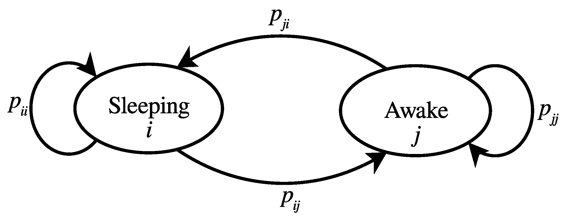
which represents the fact that, when a current state i is given at the time step k, the next state j is conditionally independent of the past states, noted as $p_{ij}\left(k\right)$. At a discrete time step k, a transition probability matrix (TPM) with the size of $N\left(k\right)\times N\left(k\right)$ can be created, where $N\left(k\right)$ represents the number of states at the time step k. Each entry in the matrix represents the change probability between two states. The sum of the transition probability of a particular state to other states equals 1, i.e., ${\sum }_j{p}_{ij}\left(k\right)=1$. For example, the Markov chain of sleeping may have two possible states $S=\{sleeping,awake\}$, and the possibility of moving from one state to another is determined by the transition probabilities, p (see Figure 2). Therefore, if a person is sleeping, there is a probability of $p_{ij}$ that, in the next time interval, (s)he will be awake; or there is a probability of $p_{ii}$ that, in the next time interval, (s)he will still be sleeping. Likewise, there are two possible transitions from awake. The corresponding TPM is

$$TPM=\left[\begin{array}{cc}{p}_{ii}& p_{ij}\\ p_{ji}& p_{jj}\end{array}\right].$$

(2)

We now describe how to estimate the transition probabilities from a time step k to its next time step $k+1$ with an empirical data set. The transition probability from a state i to j can be estimated by

$$p_{ij}\left(k\right)=\frac{n_{ij}(k+1|k)}{n_i\left(k\right)},$$

(3)

where $n_{ij}(·)$ represents the count of users whose activity has changed from i to j in the TUS data, and $n_i(·)$ represents the count of users whose activity is i at the time step k.

However, at some time step, if no transition was found between two states in the empirical data, e.g., due to the lack of some data points, $n_{ij}$ will be zero. The transition matrix will become sparse. A zero value will lead to no activity transition between the two states during data generation, which is not the case in reality. We, therefore, use Laplace smoothing to cope with the zero-frequency problem, which increases the number of each transition by one so that there is no transition with zero probability, i.e.,

$$p_{ij}^{\prime }\left(k\right)=\frac{n_{ij}(k+1|k)+1}{n_i\left(k\right)+N\left(k\right)}.$$

(4)

Note that the Laplace smoothing method is intended to exclude the zero transition probability of two states, but cannot guarantee adequacy.

Example 1 (Creating transition probability matrix).

To train activity models using our TUS data (detailed in Section 5), we combine the activities into eight categories, each of which corresponds to a state in the Markov chain (see Table 2). As activities are time-dependent, we generate a total of 143 transition matrices based on our TUS data. The TUS data were collected for every 10 min, and have 144 time steps in total (see Figure 3). We assume that the potential states remain the same in all time steps, i.e., $N\left(k\right)=8,k=1,2,\dots ,144$.

After the transition probability metrics are created with TUS data, we need to create probability density functions (PDFs) for each of the states. These PDFs are used to determine the duration of a started activity from each time step. We use Kernel Density Estimate to calculate the PDFs on the empirical data. Mathematically, a kernel is a positive function $K(x;h)$ controlled by the bandwidth parameter h [23]. With this kernel function, the density estimate to a point x within a group of points $x_i;i=1\dots N$ is defined as:

$$f_k\left(x\right)=\frac{1}{Nh}\sum _{i=1}^{N}K\left(\frac{x-x_i}{h}\right),$$

(5)

where K is the selected kernel function, $x_i$ is the point that falls in that state, and the bandwidth h is a smoothing parameter controlling the trade-off between bias and variance in the result. In this study, we use Gaussian kernel as the density function to fit the duration distribution of a state. However, note that there are other kernels available. For example, a binned kernel density function can be a better option when the size of points, N, is big.

Example 2 (Activity duration distribution).

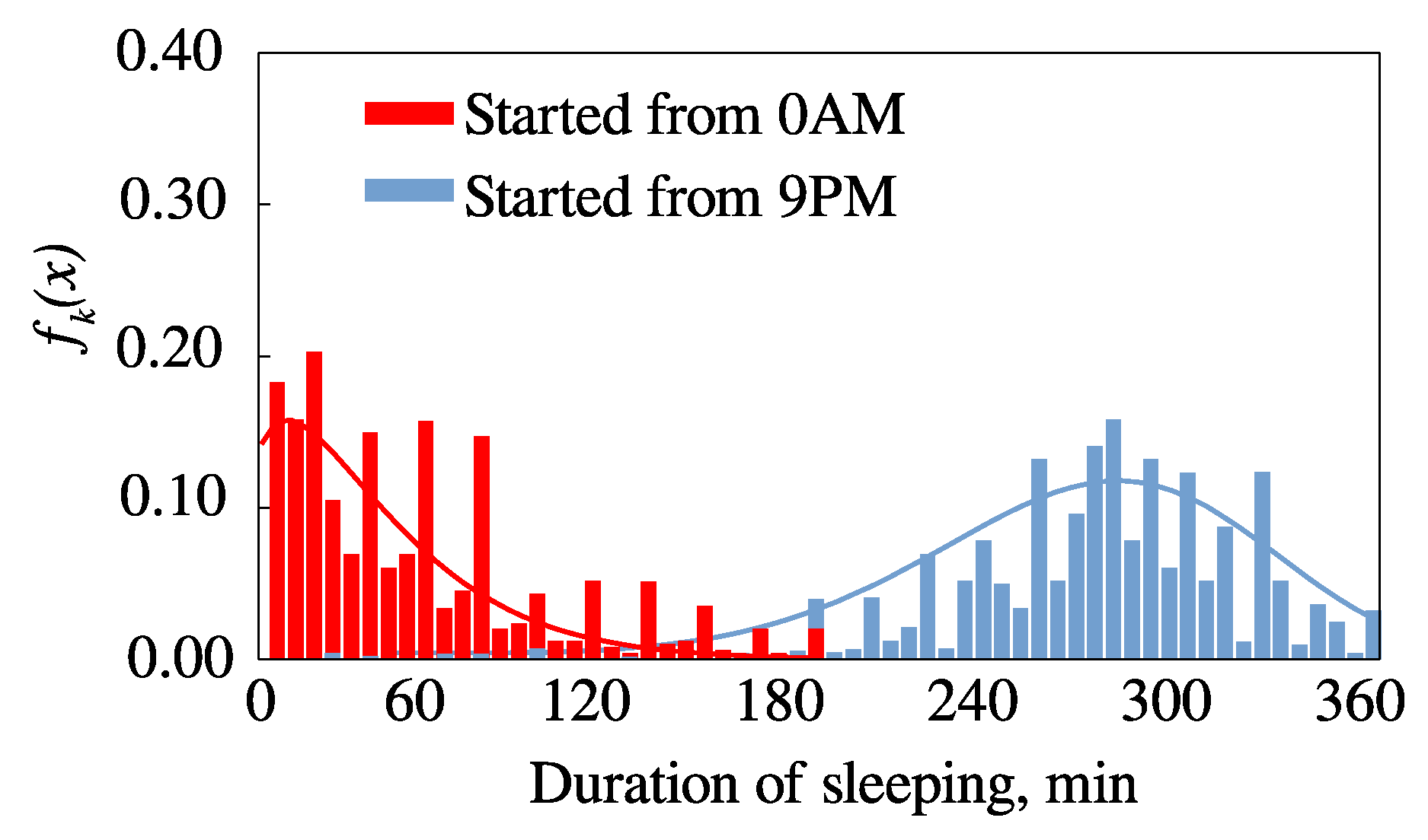
Figure 4 shows the examples of sleeping activities that started at 9:00 p.m. and 12:00 a.m., respectively, which are fitted by Gaussian distribution. The figure shows that the highest probability of the sleeping duration is 0–60 min for beginning to sleep from 12:00 a.m., and 240–300 min for starting to sleep from 9:00 p.m.

4.2. Generating an Individual Activity Sequence

We start to generate an activity sequence when the Markov chain model parameters and the PDFs are ready. The generation involves a random walk on the Markov chain. We first pick an initial state according to the probability of the time-use data at a specified starting time, then a subsequent state is picked based on the transition probability matrix. When a state is decided, we generate the duration of the state by sampling the corresponding PDF. Algorithm 1 describes the generation process in more detail. In this algorithm, the set of transition probability matrices $\mathcal{M}$ and the probability density functions $\mathcal{F}$ of all states at each time step are given as the input. The output is the generated activity sequence representing the pattern that will potentially lead to energy consumption. The function argument m is the length of the sequence to be generated.

In the implementation, we optimise this algorithm by pre-sampling a large number of durations using the PDF for each state at each time step (over 10000), and save the duration data in a database. When a sequence is being generated, uniform sampling is performed upon the saved data.

Algorithm 1 Generating an individual activity sequence.
1: functionGenActivitySeq($\mathcal{M}$, $\mathcal{F}$, m)
2:     $\mathcal{S}\leftarrow \varphi$	▹ Initialize an empty activity sequence
3:     $k\leftarrow 0$
4:     while $k<m$ do
5:         if k = 0 then
6:            $s\leftarrow$ Pick the initial state s
7:         else
8:            $s\leftarrow$ Generate the next state according to the k-th TPM, $\mathcal{M}\left[k\right]$
9:         $l\leftarrow$ Sample the duration of s according to the k-th PDF, $\mathcal{F}\left[k\right]$
10:         for $i\leftarrow 0,\dots ,l-1$ do
11:            if $i+k<m$ then
12:                $\mathcal{S}\leftarrow \mathcal{S}\oplus s$	▹ Append the state s with the duration of l
13:         $k\leftarrow k+i$
14:     return $\mathcal{S}$

Example 3 (Generating an activity sequence).

Figure 5 shows an example of generating an activity sequence using the models. The number in the table is the activity code described in Table 2. The duration of activity is generated by sampling based on the Gaussian probability density function, i.e., $l=3,2,4\dots$, whilst the change from an activity to the next is decided according to the probability in the TPM at the corresponding time step.

4.3. Generating Activity Sequences for Multiple Family Members

The previous section described generating an activity sequence for an individual person or a single-family household. The energy demand of a single family may well be derived from the generated sequence of activities. However, it is more complicated to simulate the activity sequences for multiple family members of a household, since some activities can demonstrate an exclusive nature between the sequences. A good example is that, if there is a couple living in a household and they are accustomed to making supper together, the cooking activity will be displayed at the same time in both activity sequences. However, if they agree that only one person is responsible for the supper, the cooking activity will appear in the activity sequence for one of them. This can be applied to other cases, such as laundry or cleaning. To simplify, this paper will focus on modelling the activities of a household with a maximum of two family members, and leave modelling more than two family members to the future work.

For the data generation, we first create a so-called independent activity sequence using the aforementioned approach for an individual person, then generate activity for the other person as a dependent sequence. The two sequences are denoted as S and $S^{\prime }$, respectively, and $S\prec S^{\prime }$ is used to express the generation order. We describe the generation of a dependent sequence $S^{\prime }$ in the following.

Definition 4 (Non-flexible Activities).

Non-flexible activities are defined as a subset of A, i.e., $\mathcal{O}\subset A$. For any individual activity, $a\in \mathcal{O}$, it appears in the activity sequence constrained by the conditions on S.

Let $\langle a^l\rangle$ represent a sequence constructed by a unique activity a that lasts for a duration of l time steps, and ⊂ denotes the containing relationship of a sequence. Therefore, the generation function will be augmented with S in order to generate $S^{\prime }$. $S[i,j]$ represents a sub-sequence of S between the time index i and j; the operator ∩ does a pair-wise joining of the activities between two sequences; and the operator $|·|$ denotes the length of a sequence. The generation process can be formalized as:

$${\mathcal{S}}^{\prime }\leftarrow {\mathcal{S}}^{\prime }\oplus \mathcal{A},$$

(6)

where ${\mathcal{S}}^{\prime }$ is the target sequence initialized by an empty sequence; $\mathcal{A}=\langle a^l\rangle$ is the generated sequence; and ⊕ is the operator of concatenating two sequences.

The generation process should meet one of the following conditions:

$$S[i,j]\cap \mathcal{A}=\left\{a\right\}\bigwedge a\in \mathcal{O},$$

(7)

$$S[i,j]\cap \mathcal{A}=\varphi \bigwedge a\in \mathcal{O},$$

(8)

$$S[i,j]\cap \mathcal{A}=\varphi \bigwedge a\in A\backslash \mathcal{O},$$

(9)

where $i=|{\mathcal{S}}^{\prime }|$ and $j=|{\mathcal{S}}^{\prime }|+|\mathcal{A}|$.

For condition (7), the non-flexible activity occurs in both sequences, and fully/partially overlaps. It can be used to simulate, for example, making food together. The condition (8) is used when the non-flexible activity should appear in ${\mathcal{S}}^{\prime }$, but may not necessarily appear in S. It can be used to simulate when the dependent family member makes food, i.e., ${\mathcal{S}}^{\prime }$, or two family members make food separately at different times. The condition (9) is used when only the independent family member makes the food, i.e., $\mathcal{S}$.

With these conditions, we now describe the generation process of the dependent sequence $S^{\prime }$ by the Algorithms 2–4 under the conditions (7), (8) and (9), respectively. The algorithms are self-explained and commented on. We suppose that the independent activity sequence $\mathcal{S}$ has been generated, and will be used as the input for the algorithms. In addition, the set of activities, A, the TPM, $\mathcal{M}$, and the probability density function of each activity at each time step, $\mathcal{F}$, is augmented to generate a dependent activity sequence.

Algorithm 2 Generate a dependent activity sequence with the condition (7).
1: functionGenDepActivitySeq(A, $\mathcal{M}$, $\mathcal{F}$, $\mathcal{S}$, $\mathcal{O}$)
2:     ${\mathcal{S}}^{\prime }\leftarrow \varphi$	▹ Initialize an empty activity sequence
3:     while $|{\mathcal{S}}^{\prime }|<|\mathcal{S}|$ do
4:         $\mathcal{A}\leftarrow \langle a^l\rangle$	▹ Generate a sub-sequence of $a,a\in A$, with duration of l using $\mathcal{M}$ and $\mathcal{F}$
5:         $i,j\leftarrow |{\mathcal{S}}^{\prime }|,|{\mathcal{S}}^{\prime }|+|\mathcal{A}|$
6:         if $a\in \mathcal{O}$ then
7:            if $S[i,j]\cap \mathcal{A}=\left\{a\right\}$ then
8:                ${\mathcal{S}}^{\prime }\leftarrow {\mathcal{S}}^{\prime }\oplus \mathcal{A}$
9:         else
10:            ${\mathcal{S}}^{\prime }\leftarrow {\mathcal{S}}^{\prime }\oplus \mathcal{A}$
11:     return ${\mathcal{S}}^{\prime }$

Algorithm 3 Generate a dependent activity sequence with the condition (8).
1: functionGenDepActivitySeq(A, $\mathcal{M}$, $\mathcal{F}$, $\mathcal{S}$, $\mathcal{O}$)
2:     ${\mathcal{S}}^{\prime }\leftarrow \varphi$	▹ Initialize an empty activity sequence
3:     while $|{\mathcal{S}}^{\prime }|<|\mathcal{S}|$ do
4:         $\mathcal{A}\leftarrow \langle a^l\rangle$	▹ Generate a sub-sequence of $a,a\in A$, with duration of l using $\mathcal{M}$ and $\mathcal{F}$
5:         $i,j\leftarrow |{\mathcal{S}}^{\prime }|,|{\mathcal{S}}^{\prime }|+|\mathcal{A}|$
6:         if $a\in \mathcal{O}$ then
7:            if $S[i,j]\cap \mathcal{A}=\varphi$ then
8:                ${\mathcal{S}}^{\prime }\leftarrow {\mathcal{S}}^{\prime }\oplus \mathcal{A}$
9:         else
10:            ${\mathcal{S}}^{\prime }\leftarrow {\mathcal{S}}^{\prime }\oplus \mathcal{A}$
11:     return ${\mathcal{S}}^{\prime }$

Algorithm 4 Generate a dependent activity sequence with the condition (9).
1: functionGenDepActivitySeq(A, $\mathcal{M}$, $\mathcal{F}$, $\mathcal{S}$, $\mathcal{O}$)
2:     ${\mathcal{S}}^{\prime }\leftarrow \varphi$	▹ Initialize an empty activity sequence
3:     $O\leftarrow \varphi$	▹ A set of non-flexible activities
4:     while $|{\mathcal{S}}^{\prime }|<|\mathcal{S}|$ do
5:         $A^{\prime }\leftarrow A\backslash O$	▹ Subtract the activity set O from A
6:         $\mathcal{A}\leftarrow \langle a^l\rangle$	▹ Generate a sub-sequence of $a,a\in A^{\prime }$, with the length of duration, l, using $\mathcal{M}$ and $\mathcal{F}$
7:         $i,j\leftarrow |{\mathcal{S}}^{\prime }|,|{\mathcal{S}}^{\prime }|+|\mathcal{A}|$
8:         if $S[i,j]\cap \mathcal{A}=\varphi \& \exists a\in S[i,j]\bigwedge a\in \mathcal{O}$ then
9:            ${\mathcal{S}}^{\prime }\leftarrow {\mathcal{S}}^{\prime }\oplus \mathcal{A}$
10:         else
11:            for each $a\in S[i,j]$ do
12:                if $a\in \mathcal{O}$ then
13:                    $O\leftarrow O\cup \left\{a\right\}$
14:     return ${\mathcal{S}}^{\prime }$

5. Implementation

The activity sequence generator is implemented as two modules. The first is an activity training module, which is implemented using Plpg/SQL programming language and the in-database machine learning library of PostgreSQL, MADlib [24]. PostgreSQL makes it easy to manipulate the data by its built-in operators, including aggregating, projecting and filtering, while MADlib offers various data analytic functions including matrix, histogram, Gaussian kernel density functions that we used in our program. The activity sequence is stored in an array-type column in PostgreSQL, and the MADlib offers many useful functions that can be directly operated on an array-type column, including aggregation, distinct, and pair-wise operational functions, which greatly ease our work. The training module only needs to run once to generate the activity models. The models are saved in the database and can be reused many times to generate activity sequences. Therefore, the performance of model training is not critically important. The second module is the data generator written in Python programming language. To generate data, the Python program will first access the database to read the models, then uses them to generate activity sequences with the additional input parameters, including the type of family (i.e., single family or multiple family members) and the number of sequences. To improve the performance, we use multi-threading programming of Python, and share the activity models across different threads. During the generation process, there is no communication between the threads. In addition, we carefully select the seed of random numbers to ensure the uniqueness of the results.

6. Evaluation

6.1. Experimental Settings and Data

We run the algorithms on a Dell Latitude E7440 laptop with a four-core Intel (R) i7 CPU, 2.1 GHz and 8 GB RAM, 256 GB SSD. This laptop is installed 64-bit Ubuntu 17.10 with 4.13.0-43-generic kernel. PostgreSQL 9.6 and MADlib 1.14 were used for the experiments.

Danish TUS data are used for the evaluation. This data set was collected by the Danish statistic office from 4679 families (17707 individuals in total) randomly extracted from administrative registers. The data set has the length of one year from March 2008 to March 2009, including 41 activities with a 10-min interval starting and ending at four o’clock in the morning. We pre-processed the data by grouping 41 activities into eight broad categories shown in Table 2. The combined activities are those being at home with the potential of using energy. The activity types with negligible effects on energy consumption or with a low frequency are grouped into others. In the following, we will evaluate the model and the performance of the algorithms based on the merged data.

6.2. Model Validation

We evaluate the model in the following five aspects: (1) statistical characteristic; (2) time-dependent characteristic; (3) state transition characteristic; (4) time series autoregression; and (5) root mean square error (RMSE).

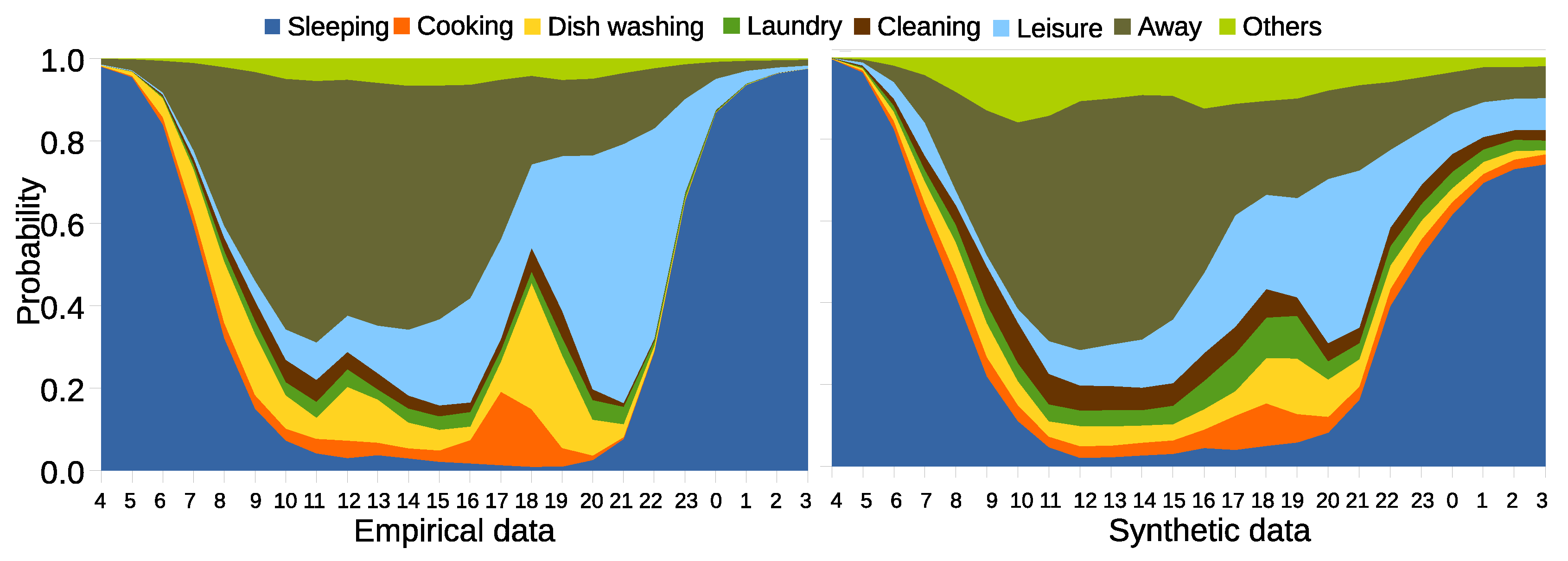
Statistic characteristic. We now first compare the quality of the empirical (real) and the generated data according to their statistical information. We generate the same amount of data for each. Figure 6 shows the activity profile at each hour of the day. The graphs show that the synthetic data can visually capture the aggregated hour-of-day patterns of the empirical data. A small difference is that the probability for each activity in the synthetic data is even more than the empirical data. This is because the Laplace smoothing method introduces a non-zero probability for the transition between any two states in the TPM.

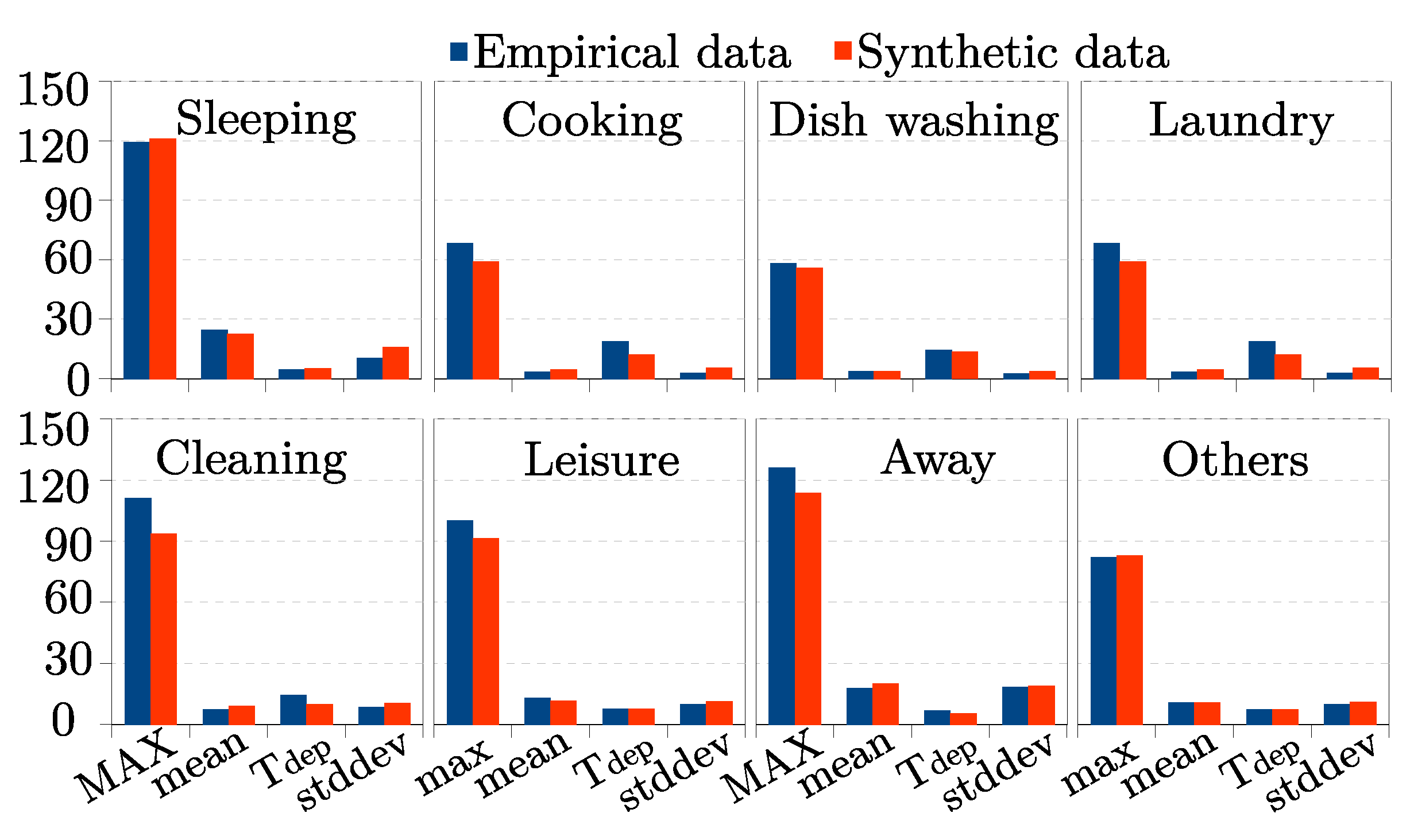
Time-dependent characteristic. Activities have time-dependence characteristics, which means that large amounts of the same practices take place at the same period of the day [25]. We now compare four quantitative metrics related to the time dependence, including MAX Distance, averaging duration, MAX Distance/average, and standard deviation. The MAX Distance is defined as

$$MAX=max((x_1-\overline{x}),\dots ,(x_n-\overline{x})),$$

(10)

where x is the duration of an activity, $\overline{x}$ is the mean of the duration, and n is the total number start practices of the activity. MAX Distance/average quantifies the time dependence of a specific activity throughout the day [25], defined as $T_{dep}=\frac{MAX}{\overline{x}}$. For example, cooking is more time-dependent than sleeping, which means that cooking mostly happens at a fixed time slot. The standard deviation is for capturing the variety of time dependence across all the days, defined as

$$\sigma \left(T_{dep}\right)=\sqrt{\frac{{\sum }_{i=1}^n{(x_i-\overline{x})}^2}{n}}.$$

(11)

The quantitative measures for the eight activities are shown in Figure 7, which indicates that the synthetic data can simulate the empirical data well.

State transition characteristic. Building occupancy is one of the most important factors that affect energy consumption in a building. Occupancy is therefore often used for energy load profiles modelling. For example, Aerts et al. [17] modelled building occupancy using three states including away, at home but awake, and sleeping as the three states are related to how energy is used in a broader category, e.g., active, inactive, or standby. We now further merge our categories into these three states and evaluate the transition probability by comparing with the real TUS data. The transition probability was computed using the same method as TPM, and they are visualized in Figure 8, instead of using a matrix. This figure reveals the time-dependent transition relation between any two of the states. For example, the top chart illustrates that during the late night and early morning people have a high probability of sleeping and staying at home, but, during the daytime, most people are not sleeping even when they are at home. The charts at the middle and the bottom can also be interpreted similarly according to the occupancy states. The charts on the left depict the occupancy transition states of the synthetic data, indicating that the model can capture the state transition characteristic from the empirical data (with a slight difference). The lines are slightly more smooth, which may be caused by the Laplace smoothing method.

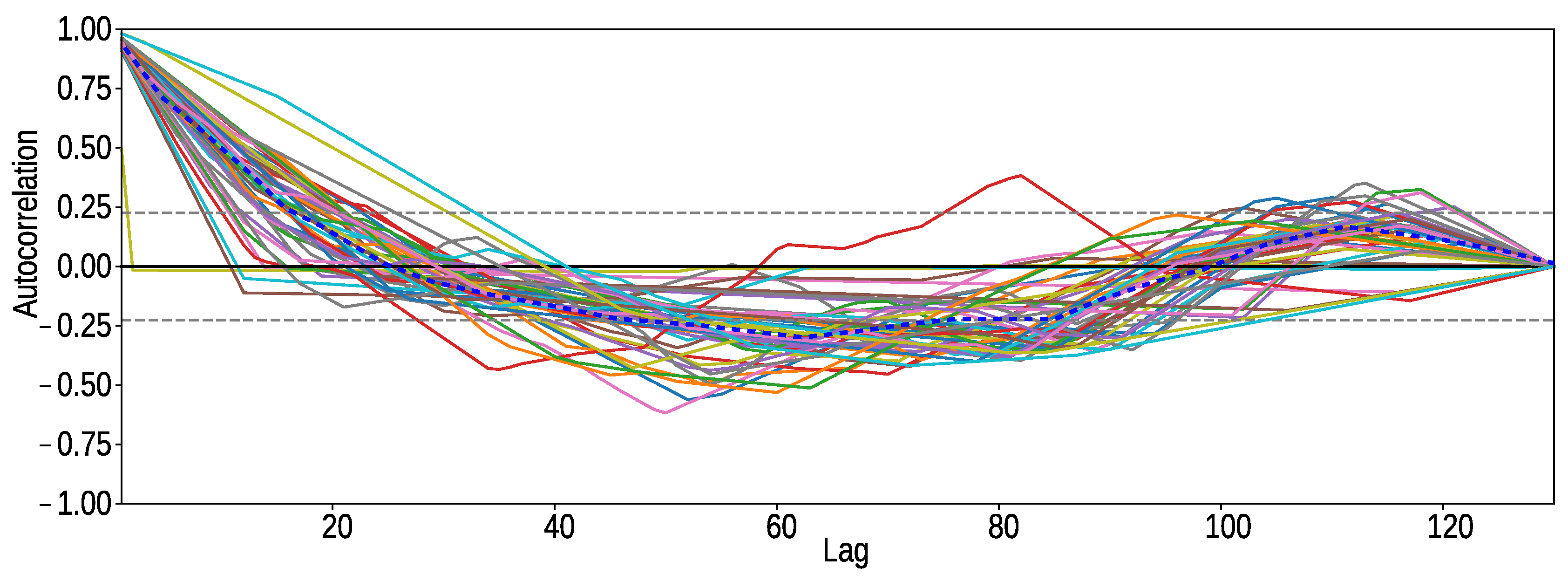
Autocorrelation. We now compute the autocorrelation of the activity profiles as time series data, which describes temporal dependencies of the activities. The activities are encoded as different state numbers according to Table 2. The autocorrelation is defined below:

$$AR\left(\mathrm{k}\right)=\frac{1}{\left|\mathrm{T}\right|-\mathrm{k}}\sum _{t=1}^{\left|T\right|-k}\frac{\left(S_t-\mu \right)\left(S_{t+k}-\mu \right)}{{\widehat{\sigma }}^2},$$

(12)

where $\left|T\right|$ is the length of a time series, $S_t$ is the encoded state at the time step t, $\mu$ is the mean value of the states, and $\sigma$ is the standard deviation.

We calculate the autocorrelations for 50 time series randomly sampled from real and synthesised data. The results are shown in Figure 9 and Figure 10, respectively, where the solid lines represent the autocorrelations for individual time series and the dashed line represents the mean of the autocorrelations. According to the results, the autocorrelation lines have a similar shape for the real and synthesised time series.

RMSE. We now verify the model by quantifying the root mean squared error (RMSE). RMSE accounts for the absolute discrepancies between the empirical data and the synthetic data generated by our model, which is defined in the following:

$$RMSE(N_s,{\widehat{N}}_s)=\sqrt{\frac{1}{\left|T\right|\times \left|S\right|}\sum _{t=1}^{\left|T\right|}\sum _{s=1}^{\left|S\right|}{(N_s\left(t\right)-{\widehat{N}}_s\left(t\right))}^2},$$

(13)

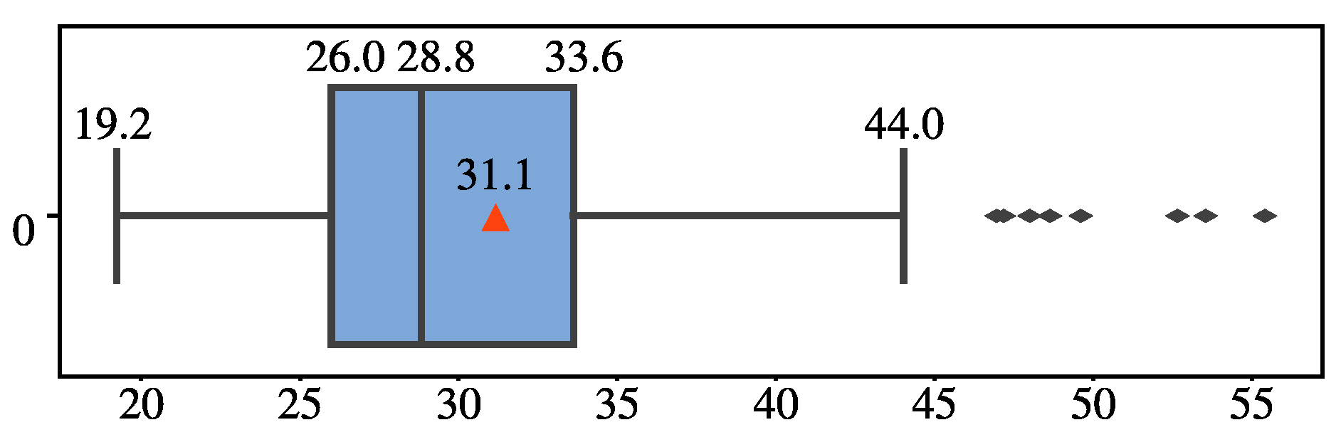
where $N_s\left(t\right)$ represents the count of state s at the t-th time step in the empirical TUS data, while ${\widehat{N}}_s\left(t\right)$ represents the count of the synthetic data; $\left|T\right|$ and $\left|S\right|$ represent the total number of time steps and the total number of states, respectively. We generate synthetic activity data for 100 times and compute the corresponding RMSE values. The resulting RMSE values are described by using the boxplot method (see Figure 11). Boxplot describes numerical data using the five parameters including lower fence, lower quartile, median, upper quartile and upper fence [26]. The length between the upper and the lower quartile is called interquartile range, $IQR$. We label the five parameters and the mean value (the red triangle) directly in the figure. According to the results, the discrepancy to the empirical data varies, due to the stochastic property of using the Markov chain method. Therefore, users can select a threshold to decide if the generated data are acceptable or not, based on the RMSE values. For example, among others using a boxplot method, the data points lie outside the lower or the upper fence (i.e., $1.5\times IQR$) are often regarded as outliers [27]. In this example, the threshold value of RMSE is 44.0 if a user has a loose requirement for the generated data.

6.3. Algorithm Performance

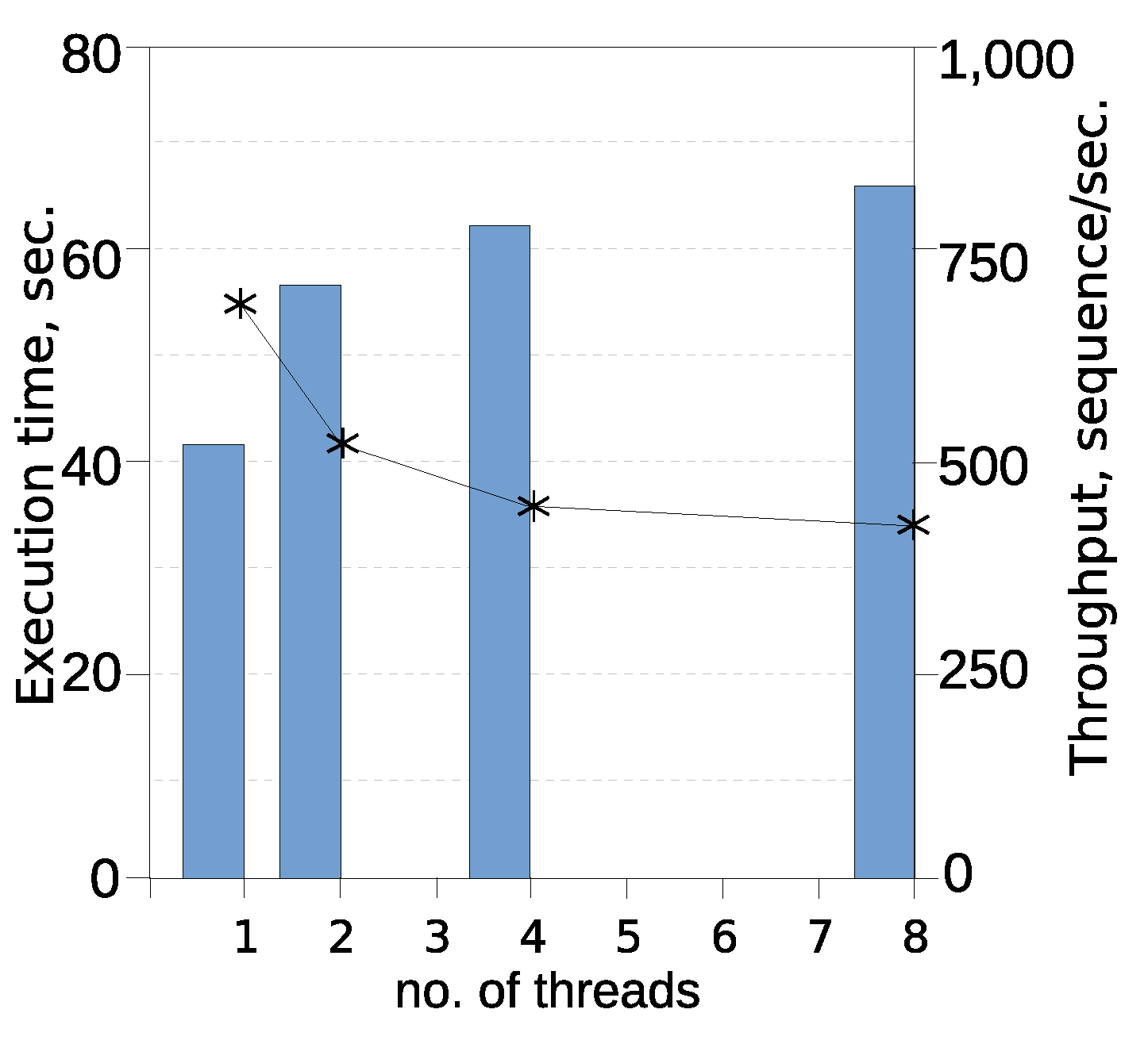
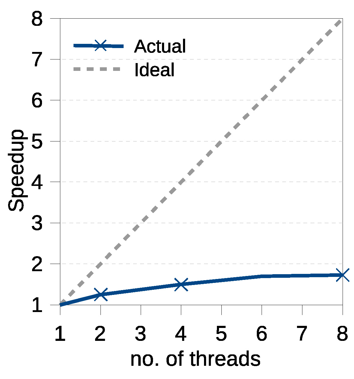
After validating the model accuracy, we now turn to evaluate the performance of running the algorithm. As mentioned earlier, the data generation model is generated once but can be re-used to generate data many times. We, therefore, only evaluate the data generation performance. As no other similar activity generators are found for the comparison, we solely report our performance. We generated 30000 activity sequences and measured the execution times when the number of threads was set to 1, 2, 4 and 8, respectively. Figure 12 shows the execution times, and the corresponding throughput. Figure 13 shows the speedup computed by the formula: $speedup=T_1/T_n$, where $T_1$ represents the execution time without enabling multi-threading, and $T_n$ represents the execution time when the number of threads is $2,4$ or 8. According to the results, the performance is improved when multi-threading is enabled, and more threads are added. In terms of speedup, it can only achieve sub-linearly. We further explored the reasons and found that this was largely due to the IO-bound for the evidence that the I/O speed became more variable when multi-threading was enabled, with a speed of 2–8 MB per second. It may, however, also be related to the CPU as the CPU usage of all the cores became 100% for running $\ge 4$ threads, and note that the experimental laptop is equipped with a 4-core CPU.

6.4. Discussion

Markov chain is a popular modelling method for system dynamics. In this paper, the model is built based on the Danish TUS data sets, for which the activities are classified into broad categories, and encoded into states to create the Markov chain model. It is often difficult to classify energy-related activities accurately. Therefore, many are categorised into others. This can affect the accuracy of using user behaviour model to estimate residential energy consumption. In addition, the TUS data capture only sequential activities of individuals, while without taking into account the parallelism for different activities and different persons. For example, one can cook but watch TV at the same time; and several people can participate in an identical activity at the same time, such as eating, watching TV or playing games. The complexity of modelling these behaviours using the Markov chain can increase exponentially. In this paper, we limit the size of family member to two and model the simplest relationship between activities. It should also be noted that activity profiles do not imply any direct relevance to load flexibility. An activity performed at different times does not mean that there is greater flexibility potential than the activity carried out at the same time of the day. For example, a dishwasher can always start at the same time, but the only requirement is to finish by the time several hours later. Moreover, the current algorithm can only generate the activity time series with a 10-min interval as the Markov model was trained by the Danish TUS data with the same time interval. However, the code can be changed accordingly if the TUS data with other time granularity are used.

As there is no standardized specification for TUS data collection, to model the activities using the TUS data from different places may involve additional manual work in data pre-processing, such as categorizing activities and defining states. To the readers who are interested in our work, we would like to open our source code at the Github repository [28]. The code can be modified and distributed under the MIT License, while the Danish TUS data used in the paper can be requested from the website [29].

7. Conclusions and Future Work

To integrate residential activities into the modelling of energy demand, we have developed a stochastic model and a data generator that can generate activity sequences for residential households. We have implemented a Markov chain and duration probability model based on a real Danish TUS data set. The presented model and algorithm can easily be reused to generate user activity data with other TUS data. We formalized the process of generating activity sequences for a household with a single family member and two family members and investigated the simulation under different boundary conditions. We have studied the robustness of the proposed model by comparing the empirical TUS data, in terms of statistical information, time-dependent property, state transition characteristics, autoregression and RMSE. We have further evaluated the performance of the data generation algorithm. The results have shown that the proposed model can generate the activity sequences that reflect actual residential user behaviours in a household, and the algorithm has good performance, with support of multi-threading.

There are several research directions for future work. First, it would be interesting to investigate how to simulate the activities of a household with more than two family members. Second, energy consumption based on activity profiles will be interesting to investigate, with additional parameters such as home appliances for better accuracy. Third, it is also interesting to study user behaviours, user thermal comfort, user interaction with heating, ventilation, and air conditioning appliances, based on the generated models.

References

1. Palacios-Garcia, E.J.; Moreno-Munoz, A.; Santiago, I.; Flores-Arias, J.M.; Bellido-Outeirino, F.J.; Moreno-Garcia, I.M. Modelling human activity in Spain for different economic sectors: The potential link between occupancy and energy usage. J. Clean. Prod. 2018, 183, 1093–1109. [Google Scholar] [CrossRef]
2. Johnson, B.J.; Starke, M.R.; Abdelaziz, O.A.; Jackson, R.K.; Tolbert, L.M. A method for modelling household occupant behavior to simulate residential energy consumption. In Proceedings of the ISGT 2014, Washington, DC, USA, 19–22 February 2014; pp. 1–5. [Google Scholar]
3. General Data Protection Regulation (GDPR). Available online: https://ec.europa.eu/commission/priorities/justice-and-fundamental-rights/data-protection/2018-reform-eu-data-protection-rules_en (accessed on 10 July 2019).
4. Santiago, I.; Lopez, M.A.; Gil-de-Castro, A.; Moreno-Munoz, A.; Luna-rodriguez, J. Energy consumption of audiovisual devices in the residential sector: economic impact of harmonic losses. Energy 2013, 60, 292–301. [Google Scholar] [CrossRef]
5. Bonke, J.; Fallesen, P. The impact of incentives and interview methods on response quantity and quality in diary-and booklet-based surveys. Surv. Res. Methods 2010, 4, 91–101. [Google Scholar]
6. Capasso, A.; Grattieri, W.; Lamedica, R.; Prudenzi, A. A bottom-up approach to residential load modelling. IEEE Trans. Power Syst. 1994, 9, 957–964. [Google Scholar] [CrossRef]
7. Muratori, M.; Roberts, M.C.; Sioshansi, R.; Marano, V.; Rizzoni, G. A highly resolved modelling technique to simulate residential power demand. Appl. Energy 2013, 107, 465–473. [Google Scholar] [CrossRef]
8. Widén, J.; Wåckelgård, E. A high-resolution stochastic model of domestic activity patterns and electricity demand. Appl. Energy 2010, 87, 1880–1892. [Google Scholar] [CrossRef]
9. Widén, J.; Molin, A.; Ellegård, K. Models of domestic occupancy, activities and energy use based on time-use data: deterministic and stochastic approaches with application to various building-related simulations. J. Build. Perform. Simul. 2012, 5, 27–44. [Google Scholar] [CrossRef]
10. Richardson, I.; Thomson, M.; Infield, D. A high-resolution domestic building occupancy model for energy demand simulations. Energy Build. 2008, 40, 1560–1566. [Google Scholar] [CrossRef] [Green Version]
11. McKenna, E.; Higginson, S.; Grunewald, P.; Darby, S.J. Simulating residential demand response: Improving socio-technical assumptions in activity-based models of energy demand. Energy Effic. 2018, 11, 1583–1597. [Google Scholar] [CrossRef]
12. Stokes, M. Removing Barriers to Embedded Generation: A Fine-Grained Load Model to Support Low Voltage Network Performance Analysis. Ph.D. Thesis, De Montfort University, Leicester, UK, 2005. [Google Scholar]
13. Paatero, J.V.; Lund, P.D. A model for generating household electricity load profiles. Int. J. Energy Res. 2006, 30, 273–290. [Google Scholar] [CrossRef]
14. Yao, R.; Steemers, K. A method of formulating energy load profile for domestic buildings in the UK. Energy Build. 2005, 37, 663–671. [Google Scholar] [CrossRef]
15. Marszal-Pomianowska, A.; Heiselberg, P.; Larsen, O.K. Household electricity demand profiles—A high-resolution load model to facilitate modelling of energy flexible buildings. Energy 2016, 103, 487–501. [Google Scholar] [CrossRef]
16. Flett, G.; Kelly, N. An occupant-differentiated, higher-order Markov chain method for prediction of domestic occupancy. Energy Build. 2016, 125, 219–230. [Google Scholar] [CrossRef]
17. Aerts, D.; Minnen, J.; Glorieux, I.; Wouters, I.; Descamps, F. A method for the identification and modelling of realistic domestic occupancy sequences for building energy demand simulations and peer comparison. Build. Environ. 2014, 75, 67–78. [Google Scholar] [CrossRef]
18. Aksanli, B.; Akyurek, A.S.; Rosing, T.S. User behavior modelling for estimating residential energy consumption. In Smart City 360; Springer: Cham, Switzerland, 2016; pp. 348–361. [Google Scholar]
19. Basu, K.; Hawarah, L.; Arghira, N.; Joumaa, H.; Ploix, S. A prediction system for home appliance usage. Energy Build. 2013, 67, 668–679. [Google Scholar] [CrossRef]
20. IRIS Data. Available online: http://ds.iris.edu/ds/nodes/dmc/data (accessed on 10 July 2019).
21. Gagniuc, P.A. Markov Chains: From Theory to Implementation and Experimentation; John Wiley & Sons: Hoboken, NJ, USA, 2017; pp. 1–235. [Google Scholar]
22. Gilks, W.R.; Richardson, S.; Spiegelhalter, D. Markov Chain Monte Carlo in Practice; Chapman & Hall: London, UK, 1996. [Google Scholar]
23. Bouezmarni, T.; El Ghouch, A.; Mesfioui, M. Gamma kernel estimators for density and hazard rate of right-censored data. J. Probab. Stat. 2011, 2011, 937574. [Google Scholar] [CrossRef]
24. Hellerstein, J.M.; Re, C.; Schoppmann, F.; Wang, D.Z.; Fratkin, E.; Gorajek, A.; Kumar, A. The MADlib analytics library: or MAD skills, the SQL. Proc. VLDB Endow. 2012, 5, 1700–1711. [Google Scholar] [CrossRef]
25. Torriti, J. Demand Side Management for the European Supergrid: Occupancy variances of European single-person households. Energy Policy 2012, 44, 199–206. [Google Scholar] [CrossRef]
26. Frigge, M.; Hoaglin, D.C.; Iglewicz, B. Some implementations of the boxplot. Am. Stat. 1989, 43, 50–54. [Google Scholar]
27. Liu, X.; Nielsen, P.S. Scalable prediction-based online anomaly detection for smart meter data. J. Inf. Syst. 2018, 77, 34–47. [Google Scholar] [CrossRef]
28. Activity Simulator. Available online: https://github.com/xiufengliu/activitysim (accessed on 10 July 2019).
29. CSSR. Available online: http://cssr.surveybanken.aau.dk (accessed on 10 July 2019).
Figure 1. Overview of residential user activity simulation.
Energies 12 03326 g001
Figure 2. An example of a Markov chain with two states.
Energies 12 03326 g002
Figure 3. The transition probability matrix in the Markov chain.
Energies 12 03326 g003
Figure 4. Examples of PDFs of sleeping, and their fitted Gaussian distributions.
Energies 12 03326 g004
Figure 5. Example of activity sequence generation.
Energies 12 03326 g005
Figure 6. Comparison between the activity profiles.
Energies 12 03326 g006
Figure 7. Comparison between time-dependence metrics.
Energies 12 03326 g007
Figure 8. Comparison of state transition.
Energies 12 03326 g008
Figure 9. The autocorrelation of the real TUS data.
Energies 12 03326 g009
Figure 10. The autocorrelation of the synthesised TUS data.
Energies 12 03326 g010
Figure 11. The boxplot of RMSE values.
Energies 12 03326 g011
Figure 12. The execution time and throughput of generating 30000 sequences.
Energies 12 03326 g012
Figure 13. The speedup of generating 30000 sequences.
Energies 12 03326 g013