Hybrid Optimization Methodology (Exergy/Pinch) and Application on a Simple Process


Abstract
1. Introduction
2. Process Improvement Methods
2.1. The Principal Methods
2.1.1. Thermodynamic Methods
2.1.2. Heuristic Methods
2.1.3. Optimization Methods
2.2. The Combined Methods
2.3. Objectives
3. Proposed Hybrid Method
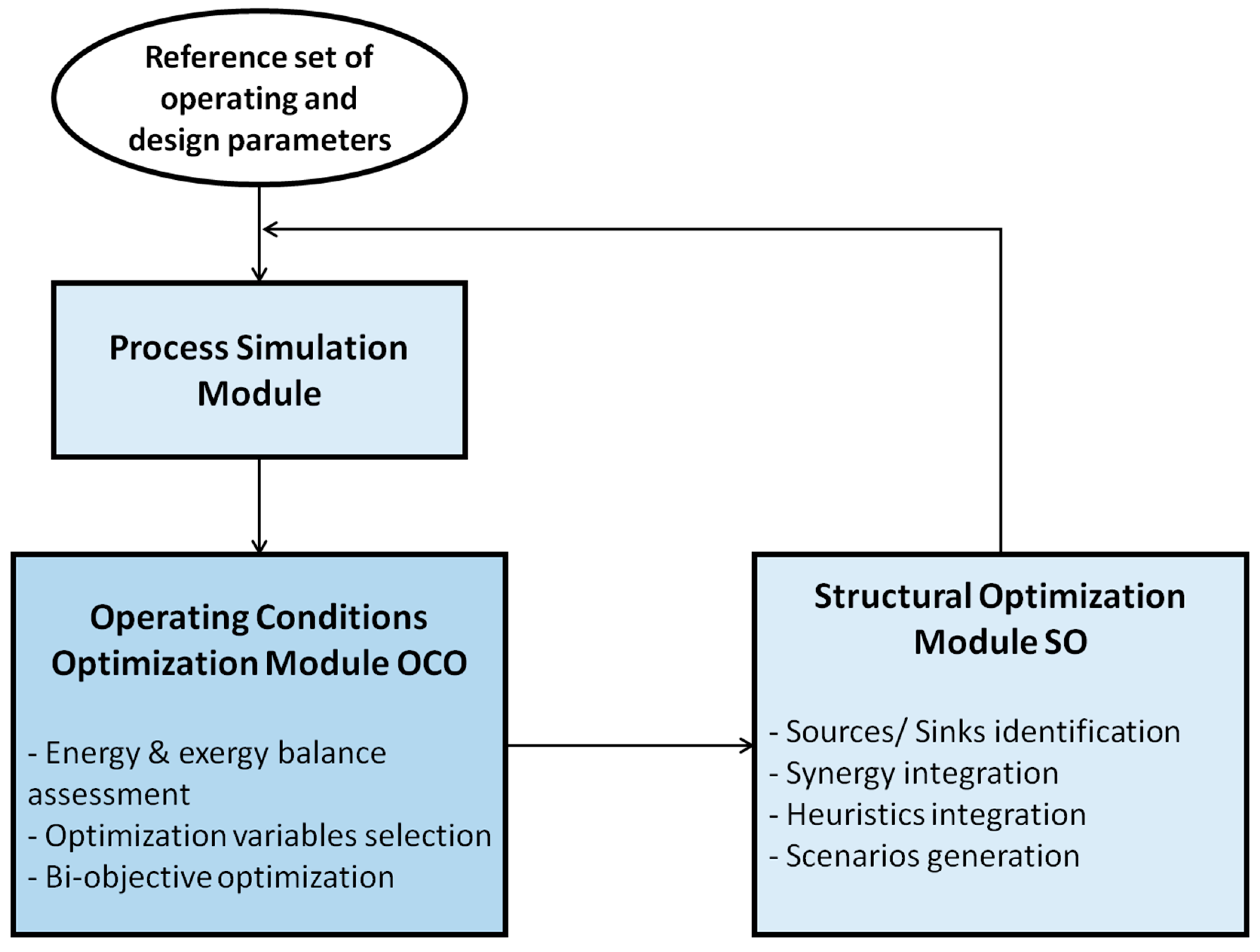
3.1. General Framework
3.2. Operating Conditions Optimization
3.2.1. Pinch Analysis Unit
- Process data extraction: The process data are first extracted including the inlet and outlet temperatures, heat loads, minimum temperature approaches, and heat exchange coefficients of the heat streams.
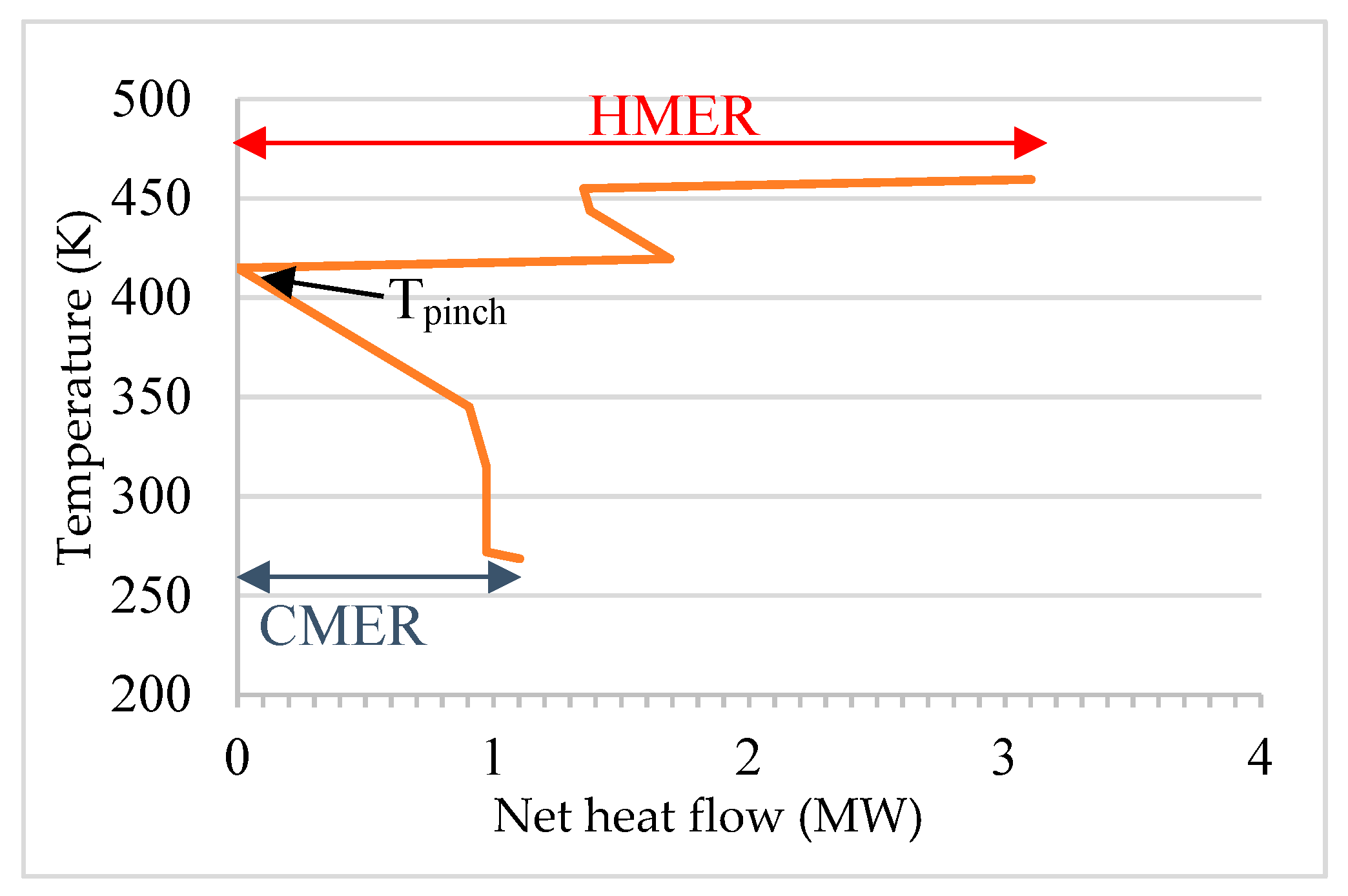
- MER calculation: The pinch temperature and the minimum energy requirements (MER) of the studied process are calculated according to the problem table algorithm given by Linnhoff and Flower [49], which is the most intelligible and uncomplicated numerical method for determining the required properties. The MER represents the external heating and cooling utilities required in a process. It indicates the remaining duties to satisfy when maximum energy is recovered from the hot and cold streams of the process.
- GCC drawing: The grand composite curve (GCC) of the process is drawn, representing the net energy need at each temperature level [12].
- HEN design: If the calculated MER are less than the actual external consumption of the process, a new simulation with a less consuming HEN can be generated to replace the original HEN in the rest of the methodological pattern application [12].
3.2.2. Exergy Analysis Unit
- -
- Cng operations or heating operations: A process flow that is cooled by rejecting heat above the ambient temperature or heated at sub-ambient temperature represent respectively available hot and cold exergy rejected without being valorized.
- -
- Effluents: Water, hot or cold gases released into the environment at high or low temperatures (for example, fumes from a heater) might contain a high thermal exergy. This exergy, if not valorized, will be lost.
3.2.3. Input Extraction Unit
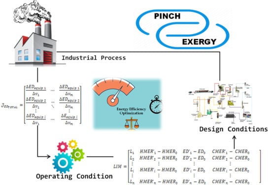
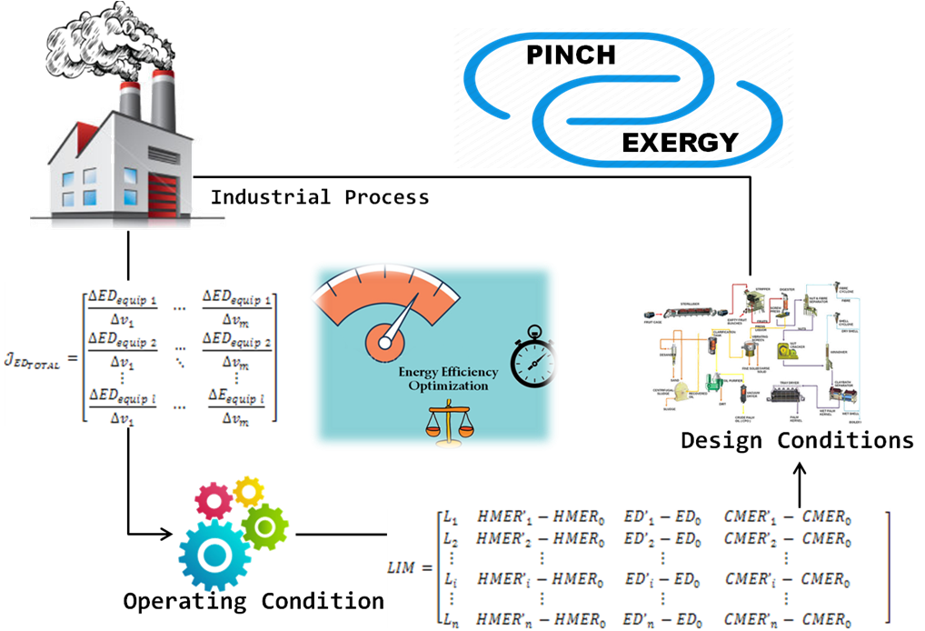
3.2.4. Jacobian Matrix Calculation Unit
- -
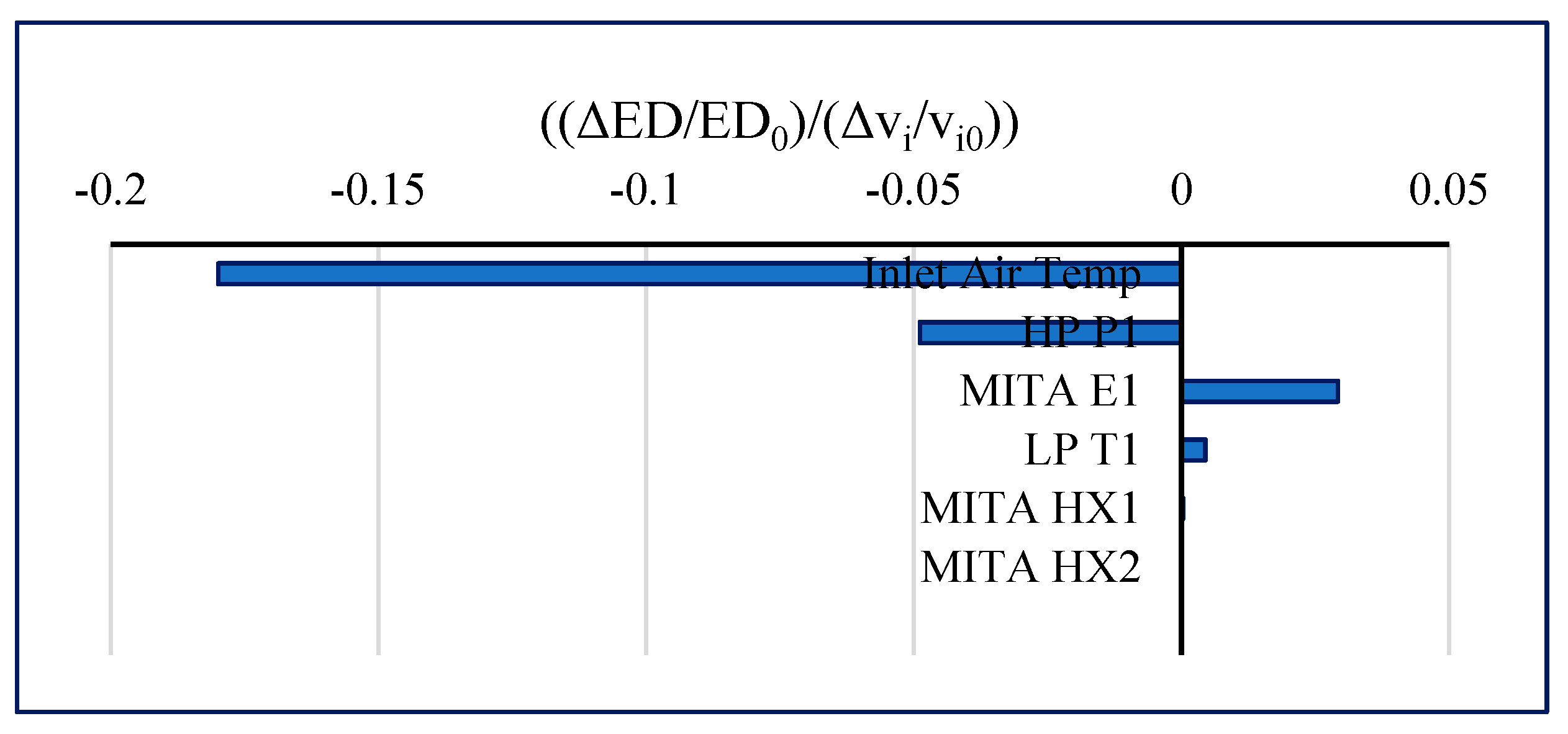
- T absolute value of the exergy destructions derivative quantifies the influence that the variable has on the exergy destruction function. The more is important, the greater is the influence of the variable on the exergy destructions and consequently a small change of this variable will bring a significant variation of the exergy destructions function and vice versa.
- -
- The sign of the derivative indicates the direction of the variation of the exergy destructions with respect to the variable . If is positive, this means that increasing the variable will increase the exergy destruction. Conversely, a negative derivative means that increasing the variable will decrease the exergy destructions.
3.2.5. Modified Simulations Sub-Unit
3.2.6. Bi-Objective Optimization Unit
3.3. Structural Optimization
- Adding new heating or cooling requirements (changes in stream temperatures) that can be supplied directly by available excess heat or heating needs through the pinch method or through thermodynamic conversion systems;
- Looking for the best thermodynamic conversion systems options helping to convert the lost exergy into a useful form;
- Changing some unitary operations into equivalent ones destroying less exergy (e.g., replacing a valve by an expander)
3.3.1. Sources/ Sinks Identification Unit
Existing Sources and Sinks
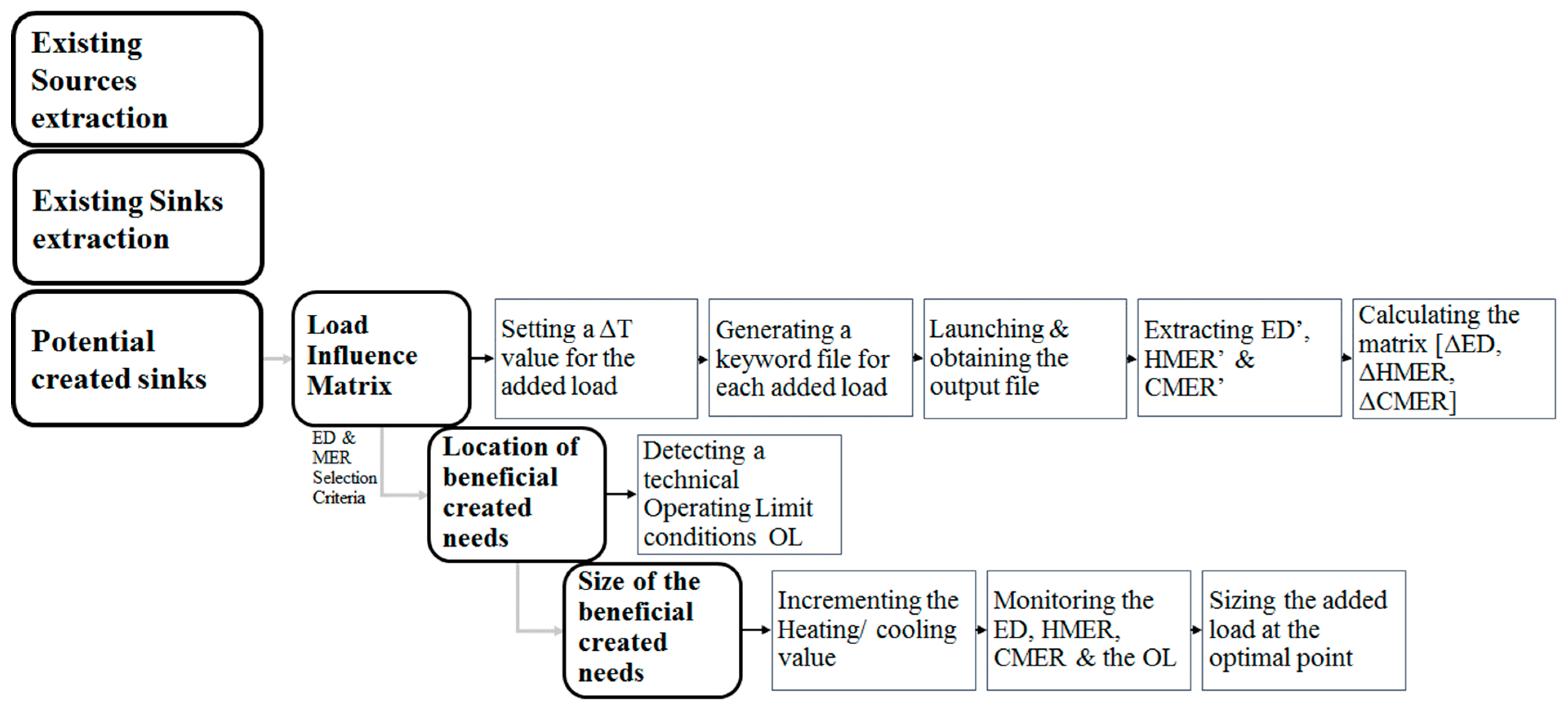
Potential Created Sinks
- -
- Specifying a value for the temperature change ΔT provoked by the added duty. To evaluate the heating influence, ΔT is positive. As for adding cooling loads, a negative ΔT is inserted.
- -
- Generating new input process simulation files each altering the input version by introducing an energy load with the specified ΔT at a different location of the process. This is modelled by a simple heat exchanger increasing or decreasing the temperature of the flow at the studied location.
- -
- Launching the generated files in order to simulate the influence of the added loads coded in each one on the global process behavior. The output file of each executed input file is obtained.
- -
- Processing each output file to extract the needed data. In fact, the exergy and energy calculators being embedded in the input simulation, a new set is evaluated corresponding to adding a load at location.
- -
- Calculating the elements of the “load influence matrix” according to Equation (12). Each line of the matrix quantifies the influence of the added load on the hot minimum energy requirements, the cold minimum energy requirements, and the total exergy destructions.
3.3.2. Synergy Integration Unit
- -
- Input Data: The algorithm uses the GCC as input data. It is automatically generated by software CERES [51] which applies the transshipment model.
- -
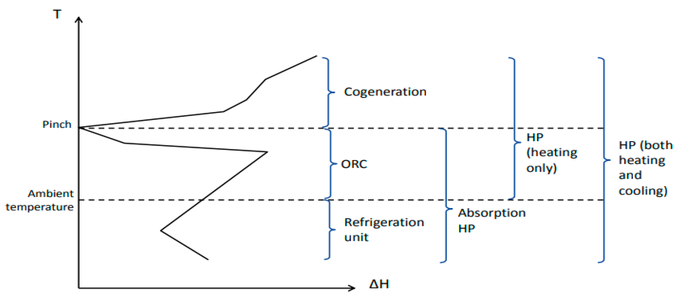
- Conversion system modeling: This preliminary step of the algorithm aims at preselecting utilities that fit the best in the process for the exergy criteria. Simplified models based on thermodynamic laws have been developed. To pre-design utilities means finding the optimal operating temperature levels for technology. Figure 5 shows a GCC covering three zones, an endothermic zone requiring heat above the pinch temperature, an exothermic zone with excess heat between the ambient, and the pinch temperatures and a refrigeration zone below the ambient. The figure illustrates the applicable conversion systems with respect to their integration zone.
- -
- Energy balance: Evaluating the total heat loads taken and provided at each temperature level after using the utilities.
- -
- GCC update: An updated GCC is rebuilt at this point of the algorithm and takes into account the effect of utilities on the process heat loads.
- -
- Electricity balance: When all utilities are set up, the electricity consumption and production has to be calculated in order to evaluate overall exergy destruction.
- -
- Restriction on utilities placement: The algorithm sets technological feasibility criterion in order to reduce the number of different technologies of utilities and accelerate the problem solving.Objective function: Energy levels [24] are used to calculate the total exergy destruction value. The last manifests as objective function to minimize.
3.3.3. Heuristic Design Modification Unit
3.3.4. Combinatory Scenarios Unit
- -
- The combined scenario includes joining single-modification scenarios each using a different availability source: in this case, no competition between the single scenarios exists and they are added together as designed in the synergy integration or heuristic modification unit.
- -
- The combined scenario includes joining single-modification scenarios sharing the same availability: In this situation, the availability and co-existing needs are assessed. If the availability suffices the new designs simultaneously, the latter are added together. However, if no disposed waste energy can provide all the single-scenarios, the combined scenario will revisit the synergy integration unit in order to redistribute optimally the disposed energy on the co-existing new designs.
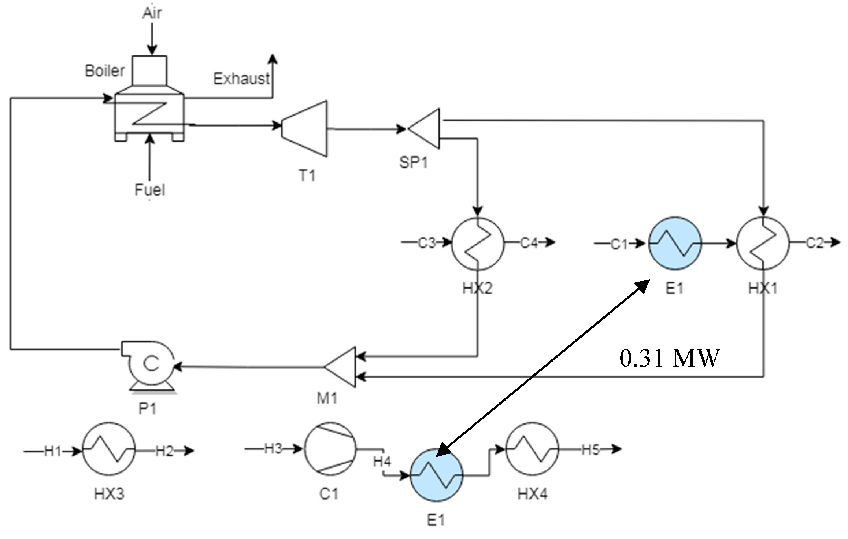
4. Case Study
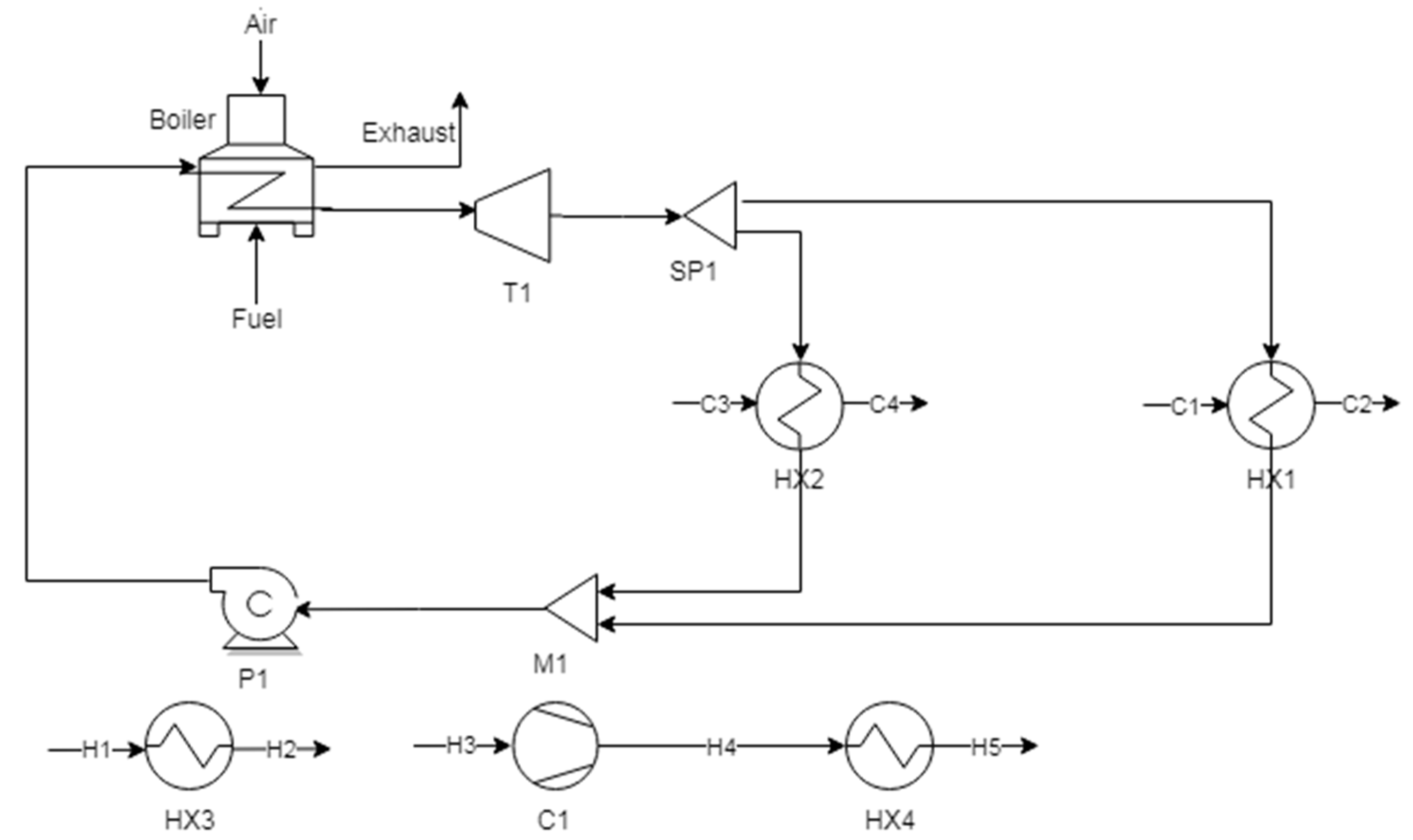
4.1. Description
4.2. OCO Module
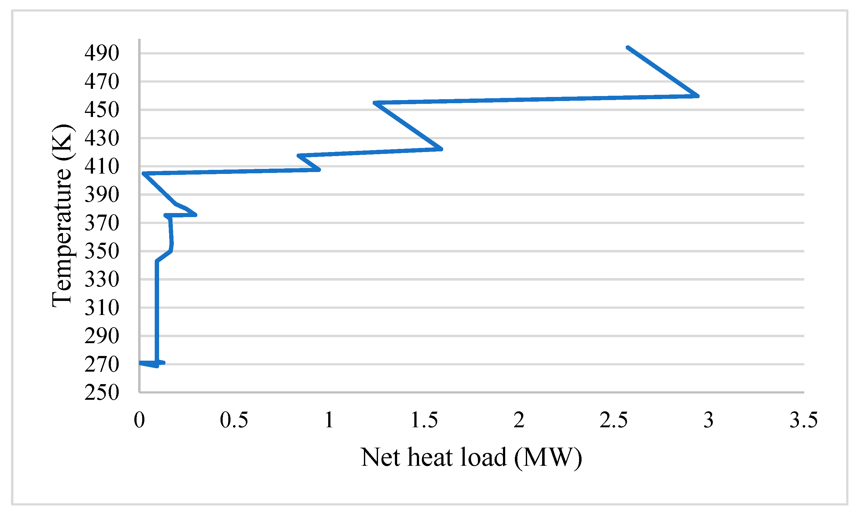
4.2.1. Pinch Analysis
4.2.2. Exergy Analysis
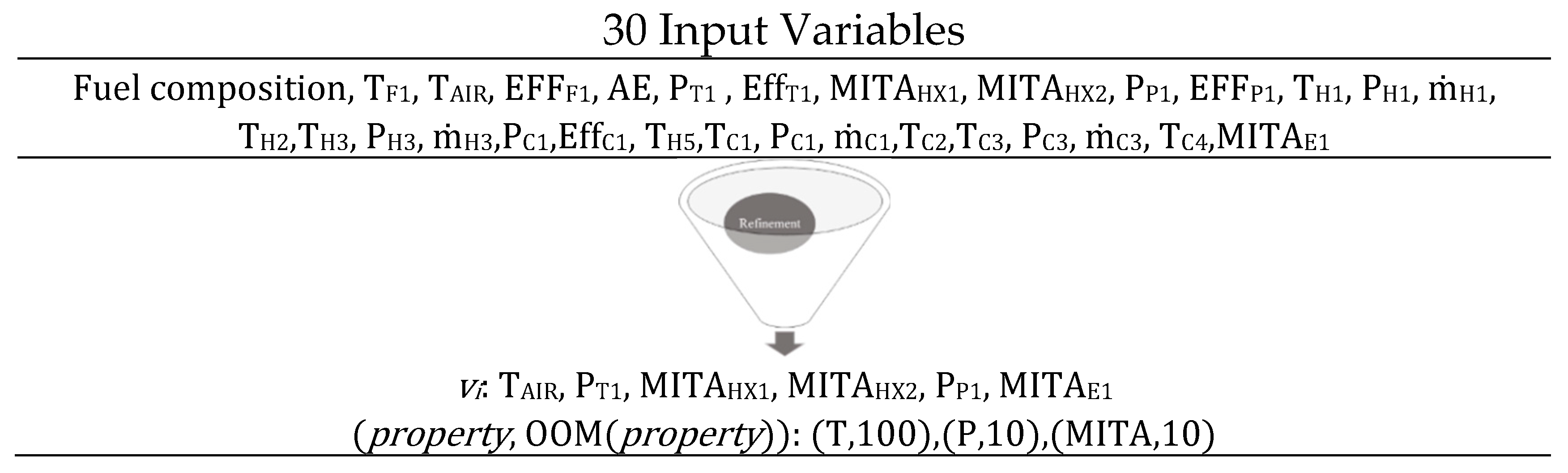
4.2.3. Input Extraction
4.2.4. Jacobian Matrix Calculation
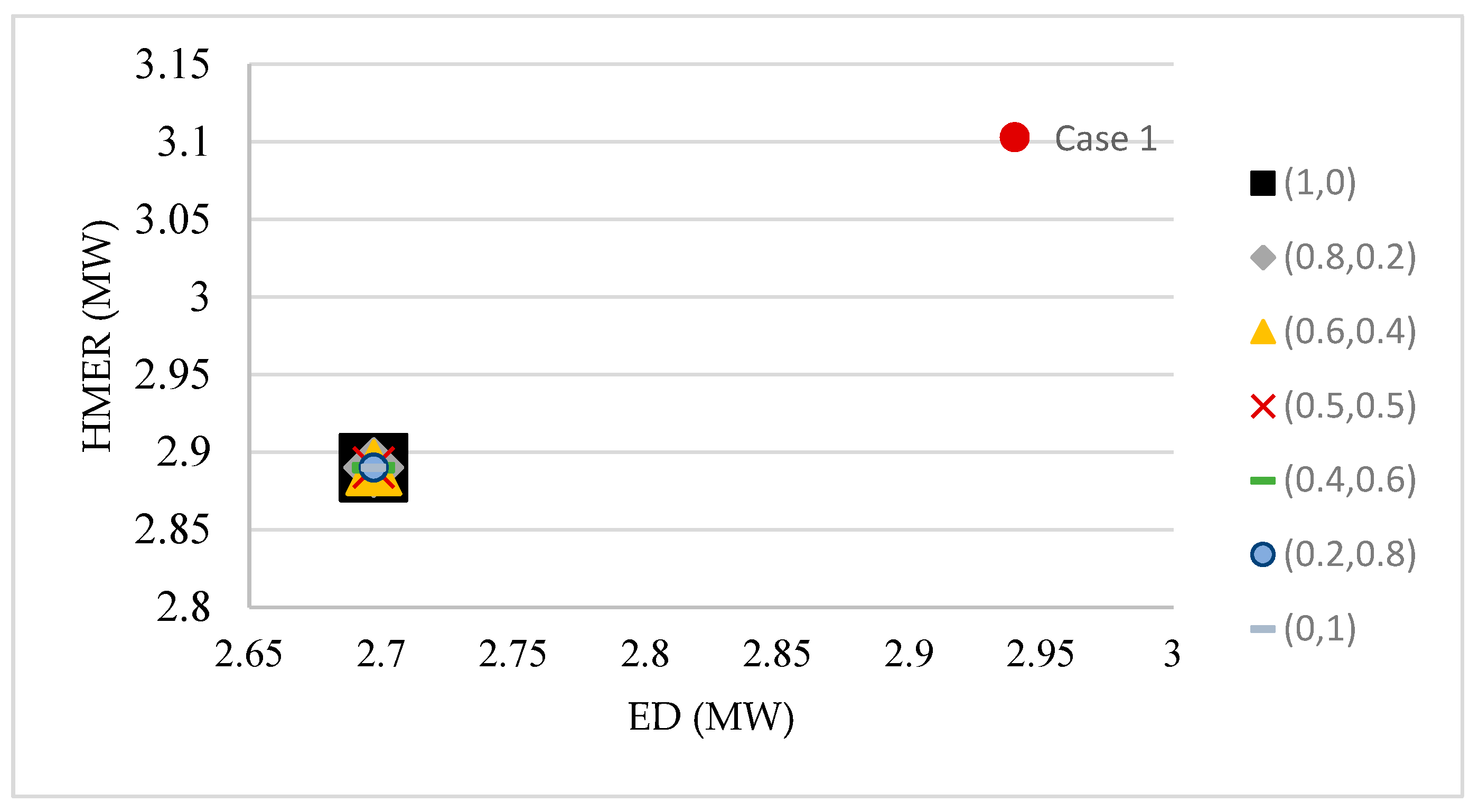
4.2.5. Bi-Objective Optimization
- -
- MITAHX1 > 3;
- -
- MITAHX2 > 3;
- -
- Tin-hot HX2 > Tout-cold HX2 + PinchHX2;
- -
- Tin-hot HX1 > Tout-cold HX1 + PinchHX1;
- -
- Liquid fraction of Pump inlet = 1.
4.3. SO Module
4.3.1. Sources/Sinks Identification
Existing Requirements and Availabilities
Added Propitious Requirements: Location and Size
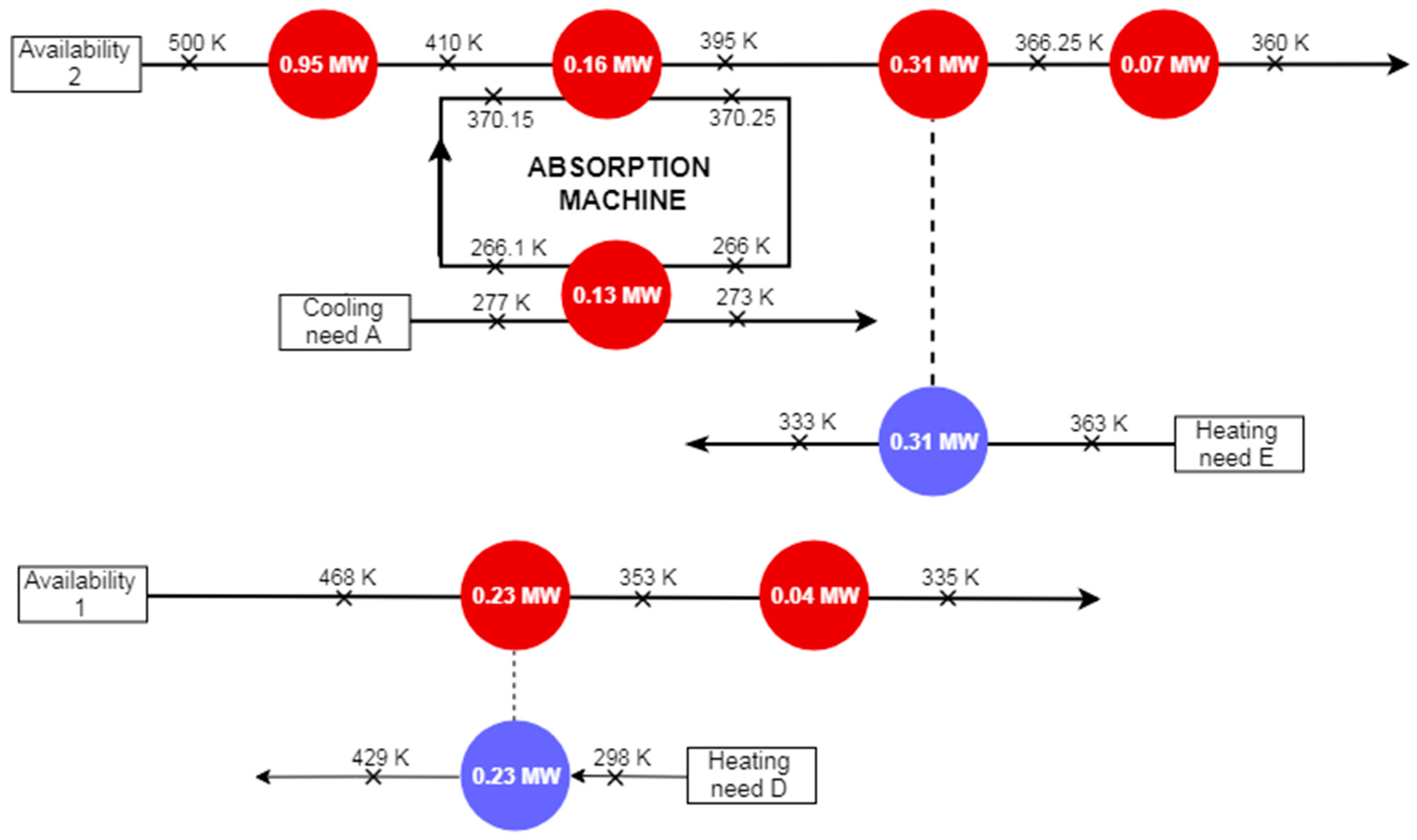
4.3.2. Synergy Integration
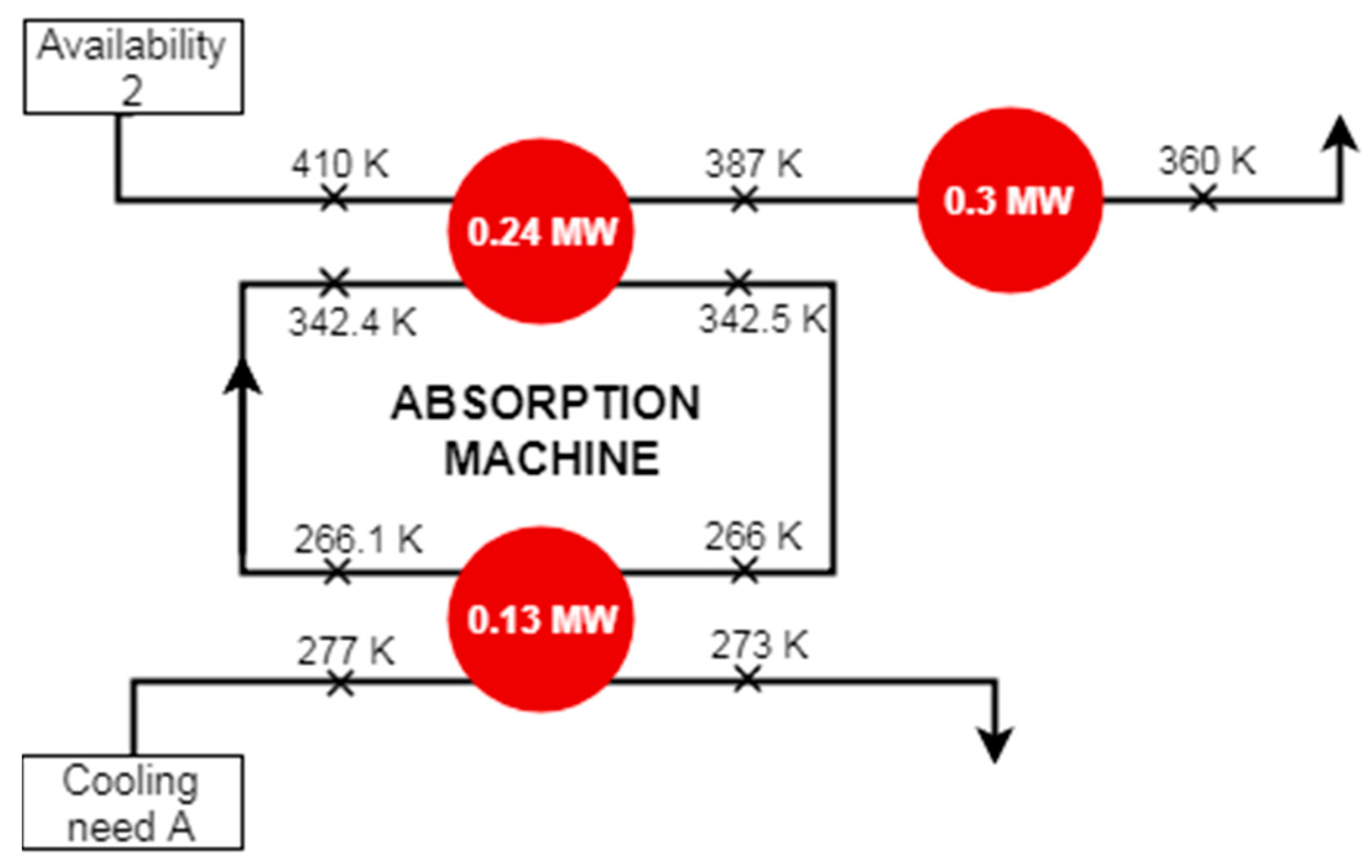
Scenario 1: Absorption Machine
Scenario 2: Combustion Air Preheater
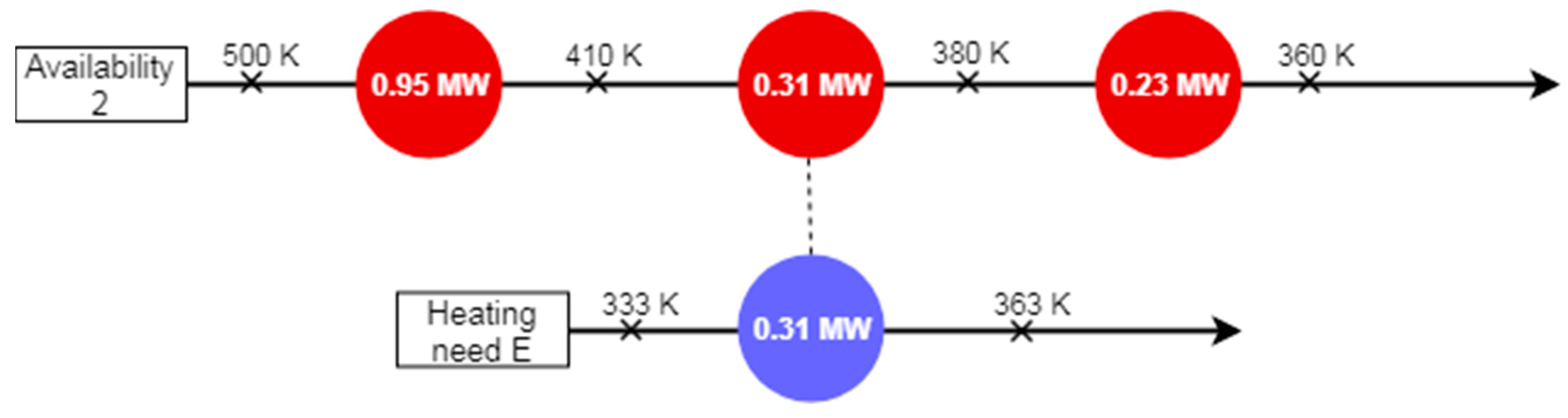
Scenario 3: Compressors’ Inlet Preheating
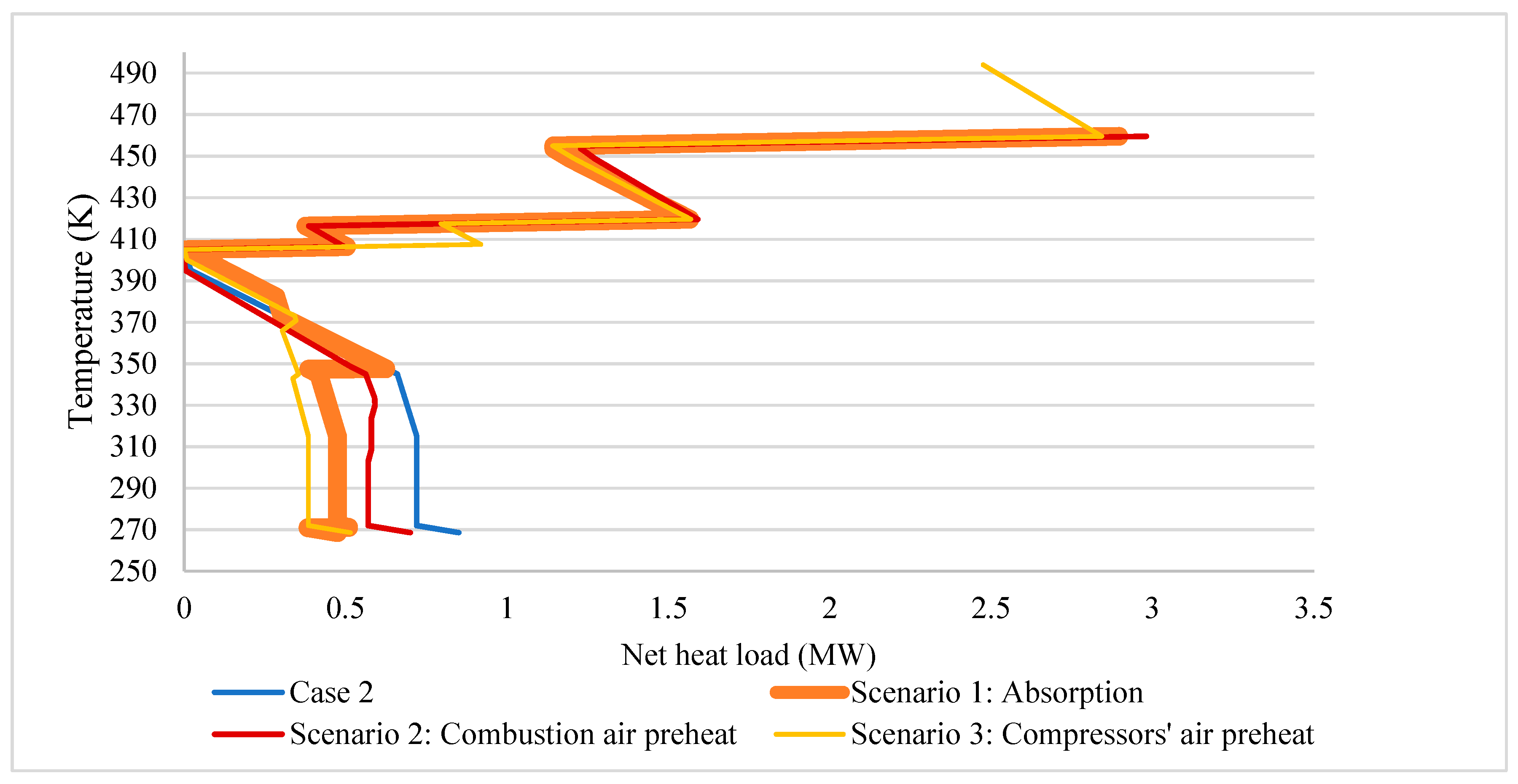
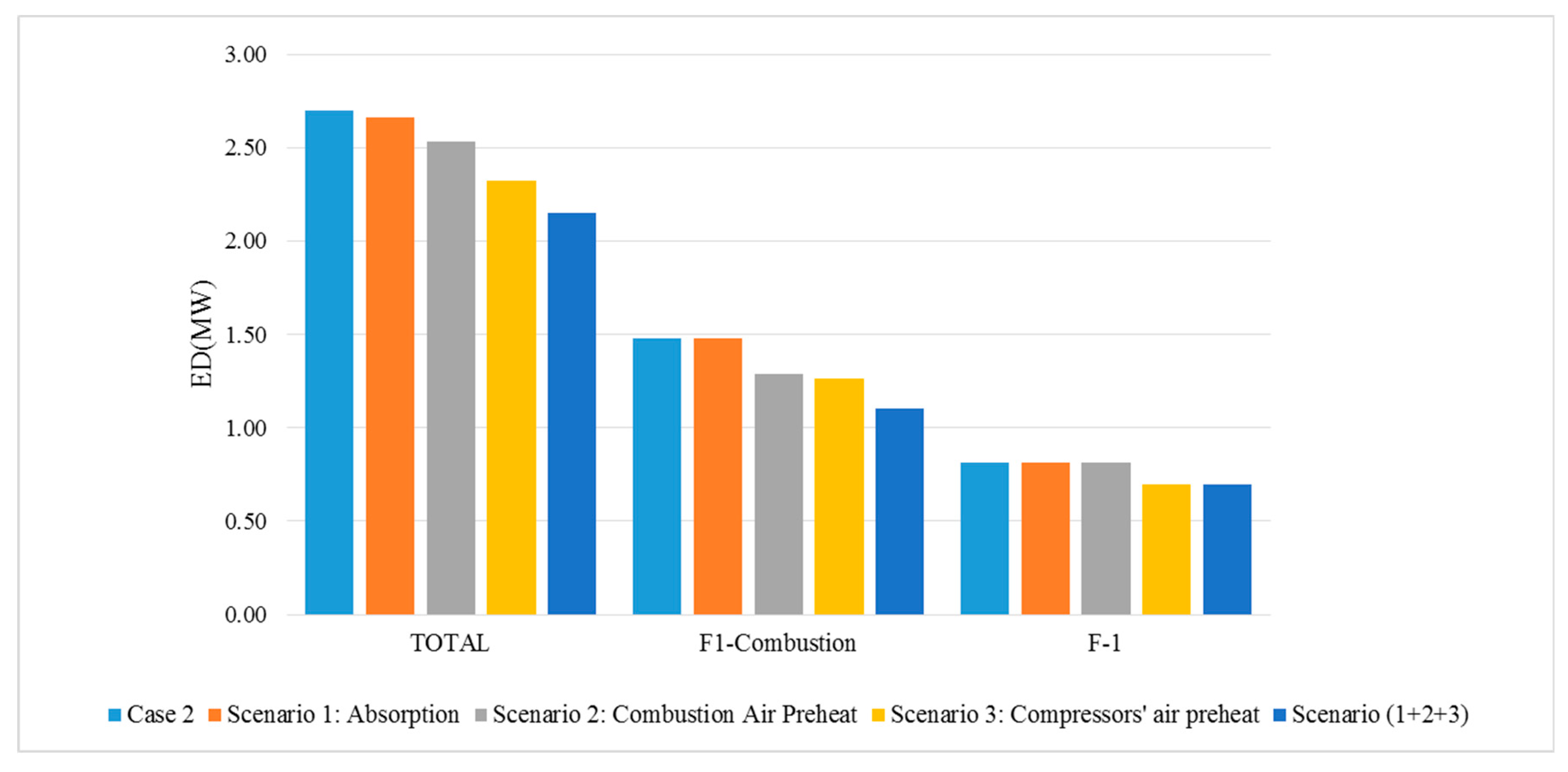
4.3.3. Combinatory Scenarios Evaluation
5. Conclusion
Author Contributions
Funding
Acknowledgments
Conflicts of Interest
Nomenclature
| Latin letters | Greek letters | |||
| CMER | Cold minimal energy required | W | Step variation value | |
| COP | Coefficient of performance | - | Infinitesimal value | |
| ΔT | Temperature change | ° | Exergy efficiency | |
| ΔTmin | Minimum temperature difference | ° | ||
| Specific exergy of a stream | J.mol−1 | Subscripts and superscripts | ||
| ED | Exergy destruction | W | c | Condenser |
| . | The desired output exergy | W | e | Evaporator |
| . | The input exergy expenses | W | i, j, n, m | index |
| Eff | Efficiency | - | min | Minimum |
| Ex | Exergy | J | ut | utility |
| Objective function | ||||
| Specific enthalpy at P, T | J.mol−1 | Acronyms | ||
| Specific enthalpy at ambient P and T | J.mol−1 | CERES | Chemins énergétiques pour la récupération d’énergies | |
| HMER | Hot minimal energy required | W | COP21 | 21st Conferences orties |
| LHV | Lower heating value | W.kg-1 | C3MR | Propane and Mixed Refrigerant |
| Mass flowrate | kg.s-1 | EGCC | Exergy Grand Composite Curve | |
| MITA | Minimum internal temperature approach | ° | FG | |
| MER | Minimal energy required | W | GCC | |
| N | Reference simulation | GHG | ||
| N’ | Optimized simulation | HEN | ||
| Mole flow rate | mol.s−1 | HP | High pressure | |
| P | Pressure | bar/bar(g) | LIM | Load influence matrix |
| Heat transfer rate | W | LNG | Liquefied | |
| s | Specific entropy at P, T | J.K−1.mol-1 | LP | Low pressure |
| s0 | Specific entropy at ambient P and T | J.K−1.mol-1 | MILP | Mixed integer linear programming |
| T | Temperature | K | OCO | Operating conditions optimization |
| T0 | Ambient temperature | K | OL | Operating limit |
| vi | Variable of the exergy destruction function | - | OOM | Order of magnitude |
| Variation number j of variable vi | - | ORC | Organic Rankine Cycle | |
| Power | W | PFD | Process flow diagram | |
| w1, w2 | Weights for scalarized optimization | - | SSO | Structural optimization |
References
- Max, R.; Hannah, R.; Esteban, O.-O. World population growth. Our World in Data. May 2019. Available online: OurWorldinData.org (accessed on 6 June 2019).
- Statistics, B.P. Statistical Review of World Energy; BP p.l.c: London, UK, 2017. [Google Scholar]
- International Energy Agency. Key World Energy Statistics; OECD/IEA: Paris, France, 2016. [Google Scholar]
- Lin, D.; Hanscom, L.; Martindill, J.; Borucke, M.; Cohen, L.; Galli, A.; Lazarus, E.; Zokai, G.; Iha, K.; Eaton, D. Working Guidebook to the National Footprint Accounts. June 2018. Available online: www.footprintnetwork.org (accessed on 16 September 2018).
- Hannah, R.; Roser, M. CO₂ and Greenhouse Gas Emissions. Our World in Data. 2017. Available online: Ourworldindata.org/co2-and-other-greenhouse-gas-emissions (accessed on 16 September 2018).
- United Nations News. UN News. November 2015. Available online: https://news.un.org/ (accessed on 16 September 2018).
- OECD Environmental Outlook. The Consequences of Inaction-Key Facts and Figures; OECD: Paris, France, 2012; Available online: www.oecd.org/env/indicators-modelling-outlooks/oecdenvironmentaloutlookto2050theconsequencesofinaction-keyfactsandfigures.htm (accessed on 22 October 2018).
- French Minister of Environment Energy and the Sea. Implementing the Paris agreement COP in action. In Proceedings of the Ministère de l’Environnement, de l’Energie et de la Mer, Paris, France, 30 November–12 December 2015. [Google Scholar]
- Frangopoulos, C.; Von Spakovsky, M.R.; Sciubba, E. A Brief Review of Methods for the Design and Synthesis Optimization. Int. J. Appl. Thermodyn. 2002, 5, 151–160. [Google Scholar]
- Abtin, A.; ChangKyoo, Y. Combined pinch and exergy analysis for energy efficiency optimization in a steam power plant. Int. J. Phys. Sci. 2010, 5, 1110–1123. [Google Scholar]
- Linhoff, B.; Hindmarsh, E. The Pinch Design Method for Heat Exchanger Network. Chem. Eng. Sci. 1982, 38, 745–763. [Google Scholar] [CrossRef]
- Kemp, I.C. Pinch Analysis and Process Integration; Elsevier: Amsterdam, The Netherlands, 2007. [Google Scholar]
- Beninca, M.; Trierweile, J. Heat integration of an Olefins Plant: Pinch Analysis and mathematical optimization working together. Braz. J. Chem. Eng. 2011, 28, 101–116. [Google Scholar] [CrossRef]
- Linnhoff, B.; Dunfurd, H.; Smith, R. Heat integration of distillation columns into overall processes. Chem. Eng. Sci. 1983, 38, 1175–1188. [Google Scholar] [CrossRef]
- Feng, X.; Zhu, X.X. Combining Pinch and Exergy Analysis for Process modifications. Appl. Therm. Eng. 1997, 17, 249–261. [Google Scholar] [CrossRef]
- Szargut, J. International progress in second law analysis. Energy 1980, 5, 709–718. [Google Scholar] [CrossRef]
- Kotas, T. The Exergy Method of Thermal Plant Analysis; Krieger Publishing Company: Malabar, FL, USA, 1995. [Google Scholar]
- Michael, M.J.; Howard, S.N. Exergy analysis. In Fundamentals of Engineering Thermodynamics, 5th ed.; Wiley: Hoboken, NJ, USA, 2006; pp. 272–325. [Google Scholar]
- Khan, N.B.N.; Barifcani, A.; Tade, M.; Pareek, V. A case study: Application of energy and exergy analysis for enhancing the process efficiency of a three stage propane pre-cooling cycle of the cascade LNG process. J. Nat. Gas Sci. Eng. 2016, 29, 125–133. [Google Scholar] [CrossRef]
- Tchanche, B.F.; Lambrinos, G.; Frangoudakis, A.; Papadakis, G. Exergy analysis of mico-organic Rankine powercycles for a small scale solar driven reverse osmosis desalination system. Appl. Therm. Energy 2010, 87, 1295–1306. [Google Scholar] [CrossRef]
- Tirandazi, B.; Mehrpooya, M.; Vatani, A.; Moovasian, S.M.A. Exergy analysis of C2+ recovery plants refrigeration cycles. Chem. Eng. Res. Des. 2011, 89, 676–689. [Google Scholar] [CrossRef]
- Mehrpooya, M.; Jarrahian, A.; Pishvaie, M.R. Simulation and exergy-method analysis of an industrial refrigeration cycle used in NGL recovery units. Energy Res. 2006, 30, 1336–1351. [Google Scholar] [CrossRef]
- Thengane, S.K.; Hoadley, A.; Bhattacharya, S.; Mitra, S. Exergy efficiency improvement in hydrogen production process by recovery of chemical energy versus thermal energy. Clean Technol. Environ. Policy 2016, 18, 1391–1404. [Google Scholar] [CrossRef]
- Feng, X.; Zhu, X.X.; Zheng, J.P. A practical exergy method for system analysis. In Proceedings of the Energy Conversion Engineering Conference, Washington, DC, USA, 11–16 August 1996. [Google Scholar]
- Tsatsaronis, G.; Park, H. On Avoidable and Unavoidable Exergy Destructions and Investment Costs in Thermal Systems. Energy Convers. Manag. 2002, 43, 1259–1270. [Google Scholar] [CrossRef]
- Morosuk, T.; Tsatsaronis, G. How to Calculate the Parts of Exergy Destruction in an Advanced Exergetic Analysis. In Proceedings of the 21st International Conference on Efficiency, Cost, Optimization, Simulation and Environmental Impact of Energy Systems, Cracow, Gliwice, Poland, 24–27 June 2008; pp. 185–194. [Google Scholar]
- Tsatsaronis, G.; Morosuk, T. Advanced Exergoeconomic Evaluation and Its Application to Compression Refrigeration Machines. ASME Conf. Proc. 2007, 859–868. [Google Scholar] [CrossRef]
- Petrakopoulou, F.; Tsatsaronis, G.; Morosuk, T.; Carassai, A. Advanced Exergoeconomic Analysis Applied to a Complex Energy Conversion System. ASME J. Eng. Gas Turbines Power 2012, 134, 801–808. [Google Scholar] [CrossRef]
- Merriam, W. Heuristic Definition; Encyclopedia Britannica: London, UK, 2014. [Google Scholar]
- Eberle, R.F. Developing imagination through scamper. J. Creat. Behav. 1972, 6, 199–203. [Google Scholar] [CrossRef]
- Sama, D. Looking at the True Value of Steam. Oil Gas J. 1980, 78, 103–119. [Google Scholar]
- Sama, D. A Common-Sense 2nd Law Approach to Heat Exchanger Network Design. In Proceedings of the ECOS ′92, Zaragoza, Spain, 15–18 June 1992; ASME: New York, NY, USA; pp. 329–338. [Google Scholar]
- Sama, D.; Qian, S.; Gaggioli, R. A Common-sense Second Law Approach for Improving Process Efficiencies. In Proceedings of the TAIES’89, Beijing, China, 5–8 Junuary 1989; Int.l Acad. Pub: Beijing, China, 1989; pp. 520–531. [Google Scholar]
- Szargut, J.; Sama, D. Practical Rules of the Reduction of Energy Losses Caused by the Thermodynamic Imperfections of Thermal Processes. In Proceedings of the II International Thermal Energy Congress, Agadir, Morocco, 5–8 June 1995; Volume 2, pp. 782–785. [Google Scholar]
- Papoulias, S.A.; Grossmann, I.E. A structural optimization approach in process synthesis—II. Comput. Chem. Eng. 1983, 7, 707–721. [Google Scholar] [CrossRef]
- Grossmann, E. Mathemathical Methods for Heat Exchanger Network Synthesis; Engineering Design Research Center, Carnegie Mellon University: Pittsburgh, PA, USA, 1992. [Google Scholar]
- Zoughaib, A. Méthode du Pincement.; Techniques de l’ingnieur: Paris, France, 2015. [Google Scholar]
- Center for Energy and Processes. Armines, Mines ParisTech. In CERES-Chemins Energétiques pour la Récupération d’Energie dans les Systèmes Industriels; Mines ParisTech: Paris, France, 2013. [Google Scholar]
- Lee, G.C.; Smith, R.; Zhu, X.X. Optimal Synthesis of Mixed-Refrigerant Systems for Low-Temperature Processes. Ind. Eng. Chem. 2002, 41, 5016–5028. [Google Scholar] [CrossRef]
- Shirazi, M.H.; Mowla, M. Energy optimization for liquefaction process of naturam gas in peak shaving plant. Energy 2010, 35, 2878–2885. [Google Scholar] [CrossRef]
- Sanavandi, H.; Ziabasharhagh, M. Design and comprehensive optimization of C3MR liquefaction naturalgas cycle by considering operational constraints. Nat. Gas Sci. Eng. 2016, 29, 176–187. [Google Scholar] [CrossRef]
- Aspelund, A.; Berstad, D.; Gundersen, T. An Extended Pinch Analysis and Design Procedure Utilizing Pressure Based Exergy for Subambient Cooling; Elsevier: Amsterdam, The Netherlands, 2007. [Google Scholar]
- Gundersen, T.; Berstad, D.O.; Aspelund, A. Extending Pinch Analysis and Process Integration into Pressure and Fluid Phase Considerations; Sintef Energy Research: Trondheim, Norway, 2009. [Google Scholar] [CrossRef]
- Marmolejo-Correa, D.; Gundersen, T. A new procedure for the design of LNG processes by combining Exergy and Pinch Analyses. In Proceedings of the Efficiency, Cost, Optimization, Simulation and Environmental Impact of Energy Systems, Perugia, Italy, 26–29 June 2012. [Google Scholar]
- Linhoff, B.; Dhole, V. Shaft work targets for low temperature process design. Chem. Eng. Sci. 1992, 47, 2081–2091. [Google Scholar] [CrossRef]
- Juthathip, T.; Kitipat, S. Combined Exergy-Pinch Analysis to Improve Cryogenic. Chem. Eng. Trans. AIDIC 2015, 43. [Google Scholar] [CrossRef]
- Thibault, F.; Zoughaib, A.; Pelloux-Prayer, S. A MILP algorithm for heat integration in industrial processes. ECOS 2013, 75, 65–73. [Google Scholar]
- Invensys Systems Inc. PRO/II 9.3; Lake Forest, Invensys Systems Inc.: Lake Forest, CA, USA, 1994–2014. [Google Scholar]
- Flower, J.R.; Linhoff, B. Synthesis of heat exchanger networks: I. Systematic generation of energy optimal networks. AIChE J. 1978, 24, 633–642. [Google Scholar]
- Bou Malham, C.; Rivera Tinoco, R.; Zoughaib, A.; Chretien, D.; Riche, M.; Guintrand, N. A Novel Hybrid Exergy/Pinch Process Integration Methodology. Energy 2018, 156, 586–596. [Google Scholar] [CrossRef]
- Zoughaib, A.; Feidt, M.; Pelloux-Prayer, S.; Thibault, F. Chemins Energétiques pour la Récupération d’énergies (CERES); Congrès Francais de Thermique: Lyon, France, 2014. [Google Scholar]
- Zoughaib, A. From Pinch Methodology to Pinch-Exergy Integration of Flexible Systems; ELSEVIER: Amsterdam, The Netherlands, 2017. [Google Scholar]


| Eipment | Exergy Destructions | Ey eiciency | |
|---|---|---|---|
| Compressor | |||
| Turbine | |||
| Valve | |||
| Mixer and splitter | |||
| Two side exchanger (side 1 is cooling, side 2 is heating) | |||
| Condenser | |||
| Evaporator | |||
| Fired Heater | Heat exchanger | ||
| combustion | |||
| Selection Criteria | |||
|---|---|---|---|
| Heating | - | 0 | - |
| - | - | - | |
| Cooling | - | - | 0 |
| - | - | - |
| Stream | Tin (K) | Tout (K) | Load (MW) | ΔTmin/2 (K) |
|---|---|---|---|---|
| C1-C2 | 400 | 404.6 | 1.75 | 15 |
| C2-C3 | 450 | 454.6 | 1.75 | 5 |
| H1-H2 | 277 | 273.6 | 0.13 | 5 |
| H4-H5 | 458.75 | 360 | 1.06 | 15 |
| Exhaust | 475.32 | 335 | 0.31 | 20 |
| Exergy Input | Calculation Formula | MW | Exergy Destructions | MW |
|---|---|---|---|---|
| Fuel exergy | 3.91 | Combustion | 1.51 | |
| Pump electricity exergy | 0.15×10⁻² | HX Boiler | 0.97 | |
| Compressors electricity exergy | 1.31 | HX4 | 0.18 | |
| HX1 | 0.15 | |||
| Exergy Losses | C1 | 0.04 | ||
| Exhaust gas exergy | 0.19 | HX2 | 0.04 | |
| E2 | 0.02 | |||
| Exergy Output | T1 | 0.02 | ||
| Turbine work | 0.12 | HX3 | 0.00 | |
| Heat | 1.01 | P1 | 0.00 | |
| Chilled water | 0.01 | M1 | 0.00 | |
| Compressed air | 0.95 | SP1 | 00 | |
| Total | 2.94 | |||
| Availabilities & Requirements | Name | Type | T In (K) | T Out (K) | Load (MW) | Source | |
|---|---|---|---|---|---|---|---|
| Availabilities | 1 | Heat | 468.78 | 335 | 0.27 | Exhaust | |
| 2 | Heat | 410 | 360 | 0.54 | HX4 | ||
| Requirements | Existing | A | Cooling | 277 | 273 | 0.13 | Chiller water |
| B | Heating | 450 | 454.6 | 1.75 | Heating need HX2 | ||
| C | Heating | 401.4 | 404.6 | 1.23 | Heating need HX1 | ||
| Propitious Created | D | Heating | 298 | 429 | 0.23 | Combustion Air | |
| E | Heating | 333 | 363 | 0.31 | C1 Inlet Air | ||
© 2019 by the authors. Licensee MDPI, Basel, Switzerland. This article is an open access article distributed under the terms and conditions of the Creative Commons Attribution (CC BY) license (http://creativecommons.org/licenses/by/4.0/).
Share and Cite
Bou Malham, C.; Zoughaib, A.; Rivera Tinoco, R.; Schuhler, T. Hybrid Optimization Methodology (Exergy/Pinch) and Application on a Simple Process. Energies 2019, 12, 3324. https://doi.org/10.3390/en12173324
Bou Malham C, Zoughaib A, Rivera Tinoco R, Schuhler T. Hybrid Optimization Methodology (Exergy/Pinch) and Application on a Simple Process. Energies. 2019; 12(17):3324. https://doi.org/10.3390/en12173324
Chicago/Turabian StyleBou Malham, Christelle, Assaad Zoughaib, Rodrigo Rivera Tinoco, and Thierry Schuhler. 2019. "Hybrid Optimization Methodology (Exergy/Pinch) and Application on a Simple Process" Energies 12, no. 17: 3324. https://doi.org/10.3390/en12173324
APA StyleBou Malham, C., Zoughaib, A., Rivera Tinoco, R., & Schuhler, T. (2019). Hybrid Optimization Methodology (Exergy/Pinch) and Application on a Simple Process. Energies, 12(17), 3324. https://doi.org/10.3390/en12173324