Comparison of Forecasting Energy Consumption in East Africa Using the MGM, NMGM, MGM-ARIMA, and NMGM-ARIMA Model


Abstract
1. Introduction
2. Literature Review
2.1. Review of Energy Research in Africa
2.2. Review of Grey Model
2.3. Review of ARIMA Model
3. Method
3.1. MGM Model
3.2. NMGM Model
3.3. ARIMA Model
3.4. MGM-ARIMA and NMGM-ARIMA Model
3.5. The Comparison of Five Models and Formulas for Measuring Accuracy
4. Empirical Results and Discussion
4.1. Forecasting Process of MGM Model
4.2. Forecasting Process of NMGM Mode
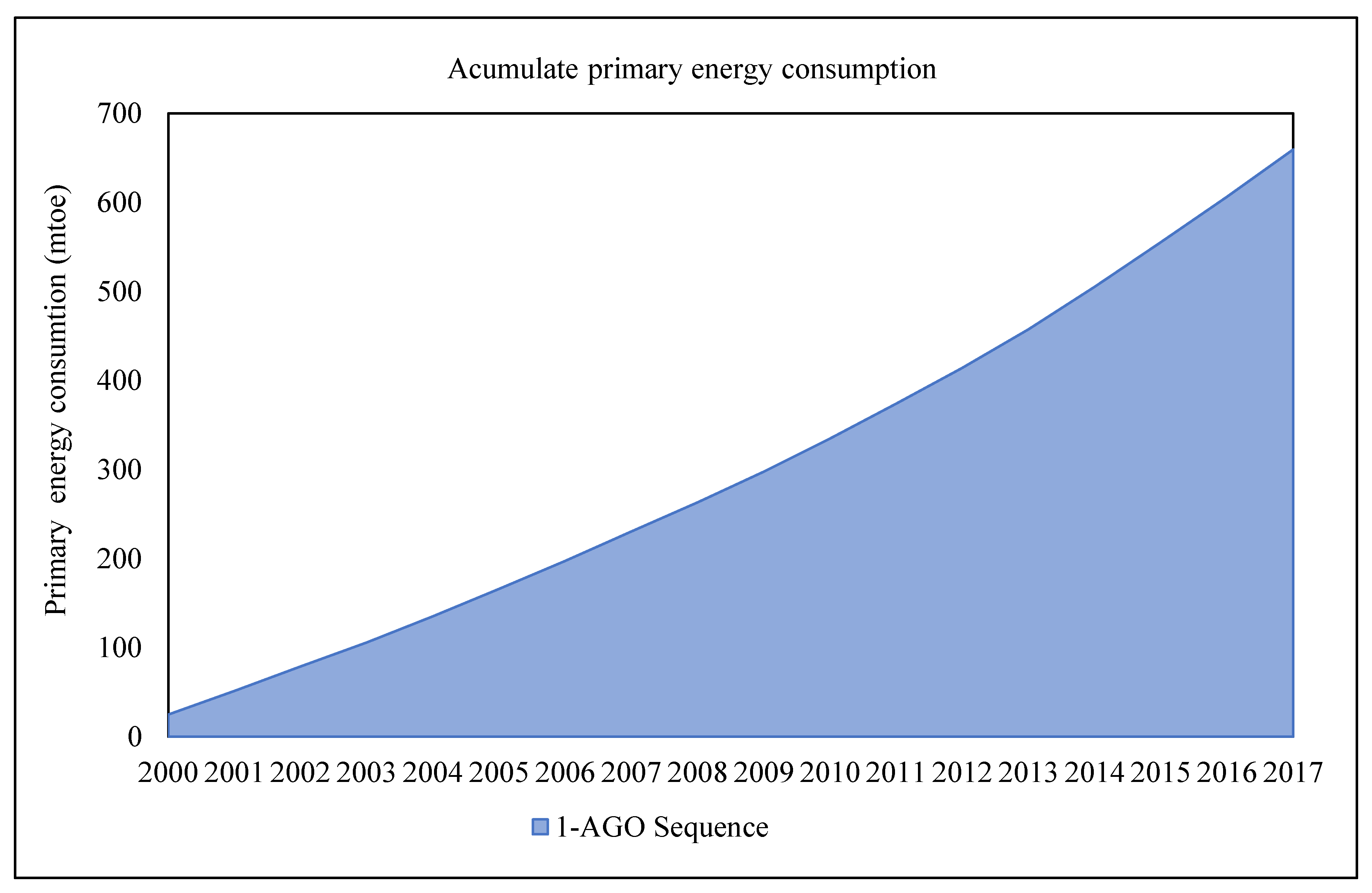
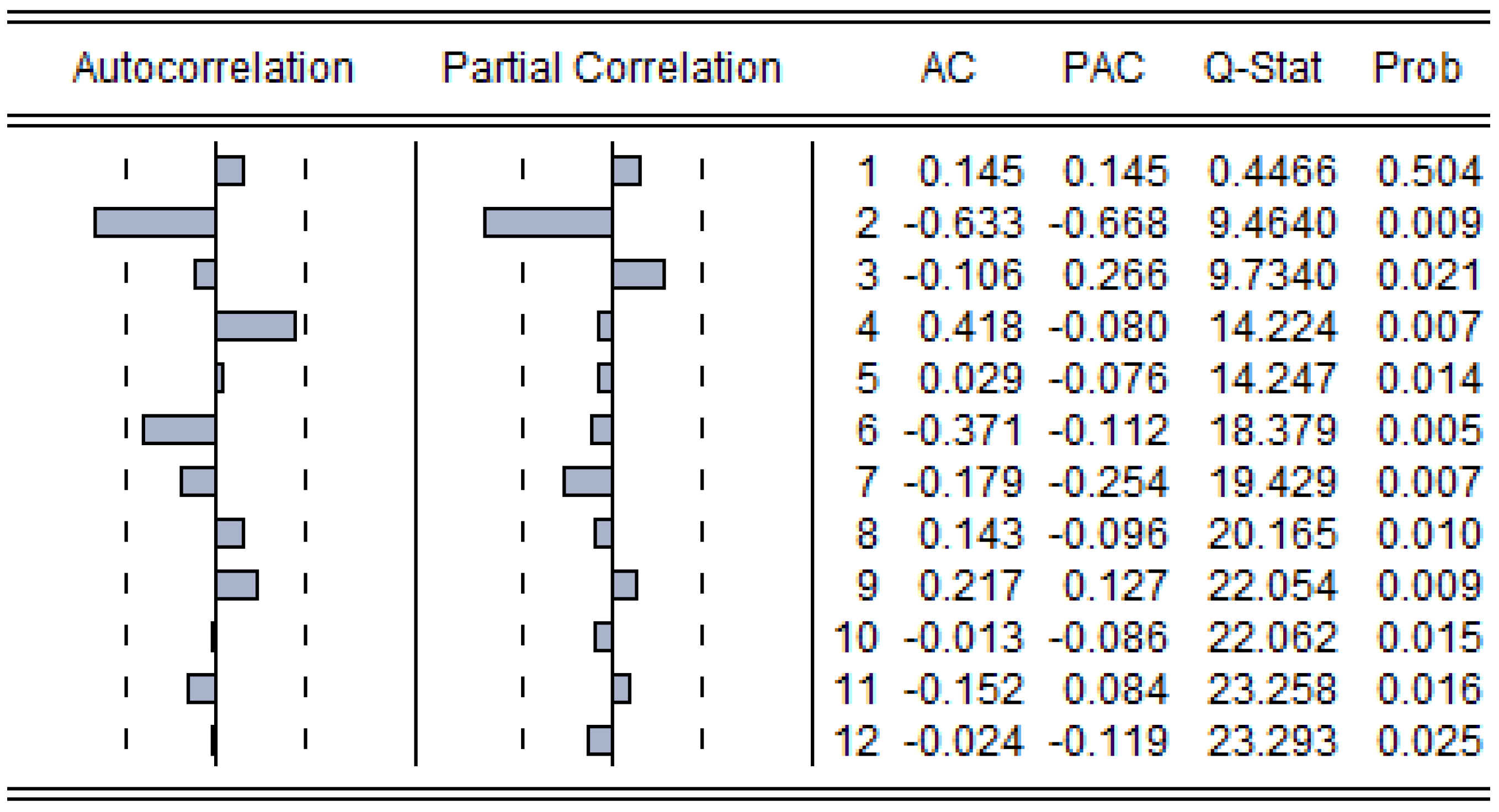
4.3. Forecasting Process of ARIMA Model
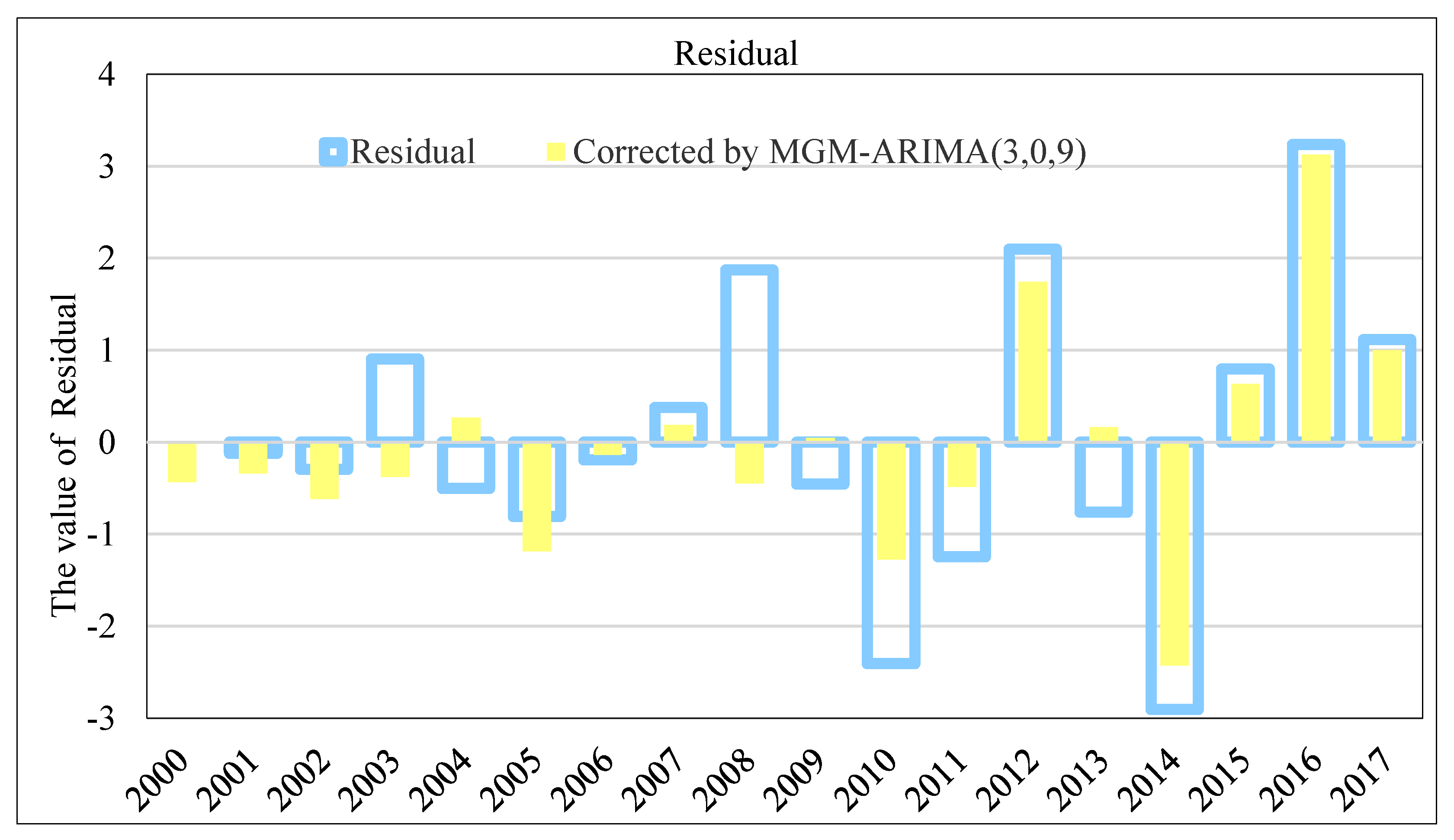
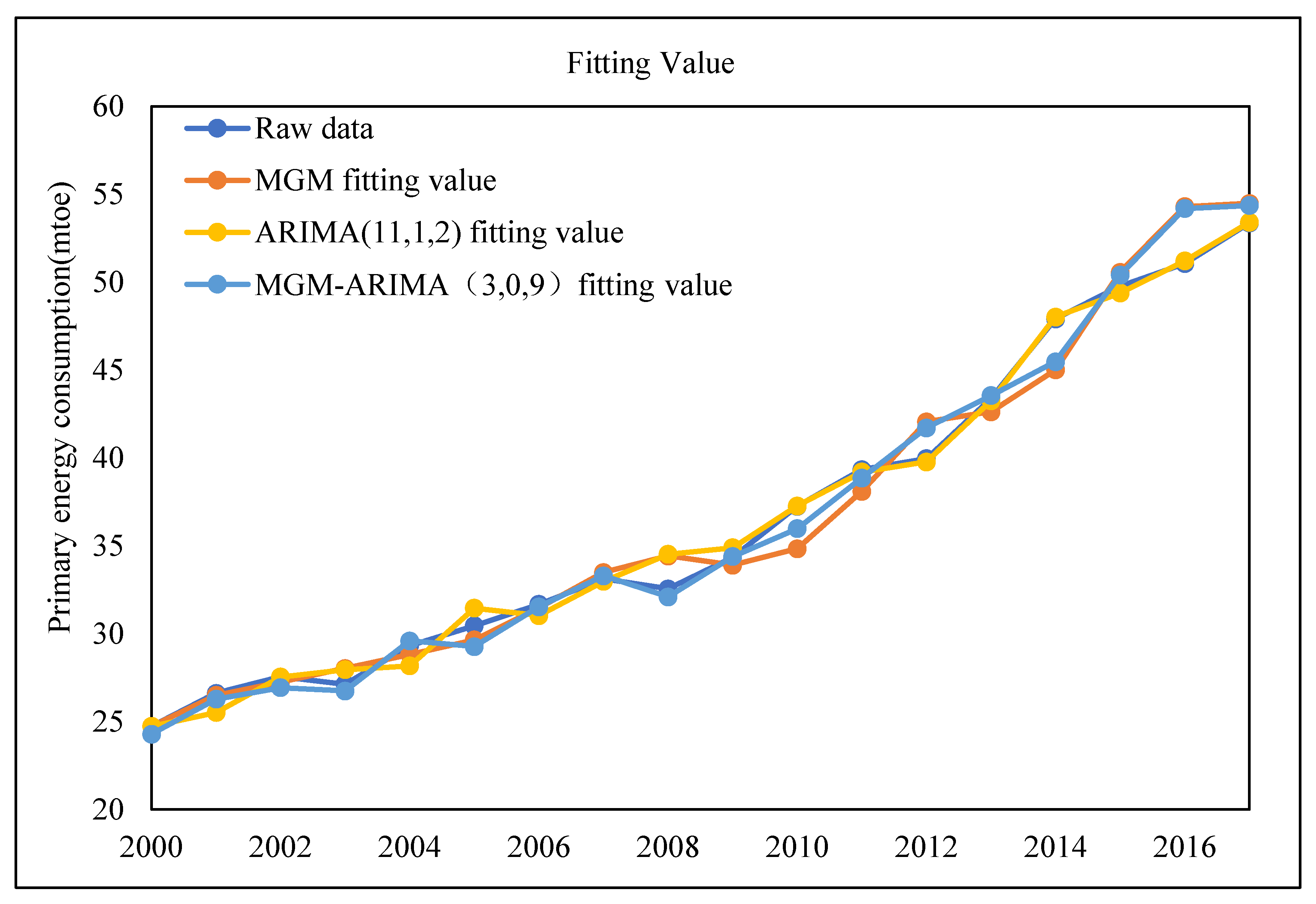
4.4. Forecasting Process of MGM-ARIMA Model
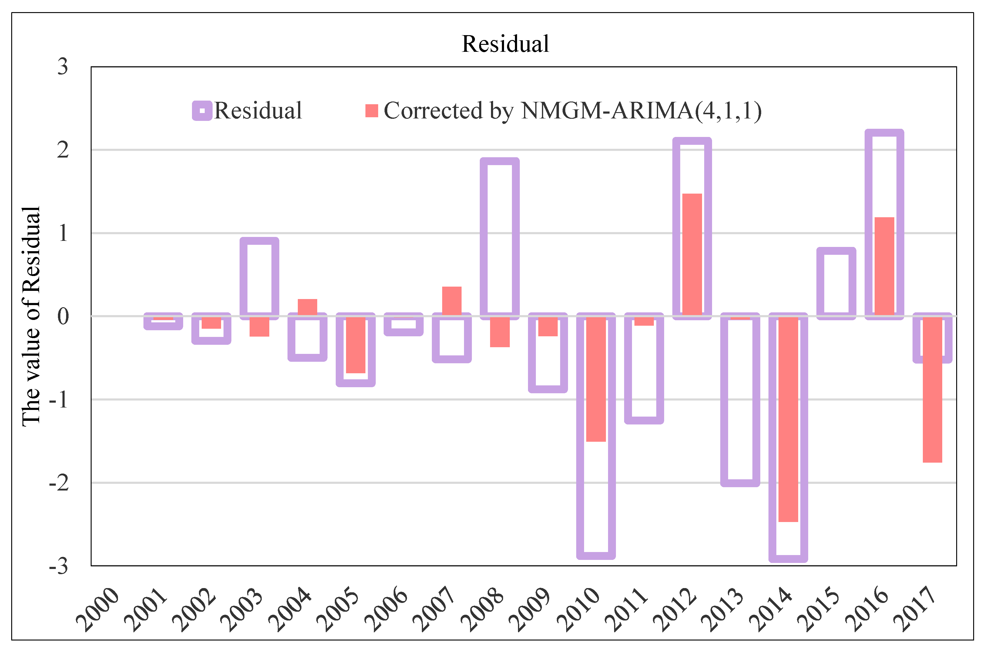
4.5. Forecasting Process of NMGM-ARIMA Model
4.6. Comparison of Fitting Results by Multiple Model
4.7. Prediction Results
5. Conclusions
Author Contributions
Funding
Conflicts of Interest
References
- Madubansi, M.; Shackleton, C. Changing energy profiles and consumption patterns following electrification in five rural villages, South Africa. Energy Policy 2006, 34, 4081–4092. [Google Scholar] [CrossRef]
- Inglesi-Lotz, R. The evolution of price elasticity of electricity demand in South Africa: A Kalman filter application. Energy Policy 2011, 39, 3690–3696. [Google Scholar] [CrossRef]
- Mulugetta, Y. Evaluating the economics of biodiesel in Africa. Renew. Sustain. Energy Rev. 2009, 13, 1592–1598. [Google Scholar] [CrossRef]
- Sokona, Y.; Mulugetta, Y.; Gujba, H. Widening energy access in Africa: Towards energy transition. Energy Policy 2012, 47, 3–10. [Google Scholar] [CrossRef]
- Sanoh, A.; Kocaman, A.S.; Kocal, S.; Sherpa, S.; Modi, V. The economics of clean energy resource development and grid interconnection in Africa. Renew. Energy 2014, 62, 598–609. [Google Scholar] [CrossRef]
- Mentis, D.; Hermann, S.; Howells, M.; Welsch, M.; Siyal, S.H. Assessing the technical wind energy potential in Africa a GIS-based approach. Renew. Energy 2015, 83, 110–125. [Google Scholar] [CrossRef]
- Ouedraogo, N.S. Modeling sustainable long-term electricity supply-demand in Africa. Appl. Energy 2017, 190, 1047–1067. [Google Scholar] [CrossRef]
- Barry, M.L.; Steyn, H.; Brent, A. Selection of renewable energy technologies for Africa: Eight case studies in Rwanda, Tanzania and Malawi. Renew. Energy 2011, 36, 2845–2852. [Google Scholar] [CrossRef]
- Schwerhoff, G.; Sy, M. Financing renewable energy in Africa—Key challenge of the sustainable development goals. Renew. Sustain. Energy Rev. 2017, 75, 393–401. [Google Scholar] [CrossRef]
- Tsikalakis, A.; Tomtsi, T.; Hatziargyriou, N.; Poullikkas, A.; Malamatenios, C.; Giakoumelos, E.; Jaouad, O.C.; Chenak, A.; Fayek, A.; Matar, T.; et al. Review of best practices of solar electricity resources applications in selected Middle East and North Africa (MENA) countries. Renew. Sustain. Energy Rev. 2011, 15, 2838–2849. [Google Scholar] [CrossRef]
- Komendantova, N.; Patt, A.; Barras, L.; Battaglini, A. Perception of risks in renewable energy projects: The case of concentrated solar power in North Africa. Energy Policy 2012, 40, 103–109. [Google Scholar] [CrossRef]
- Lacher, W.; Kumetat, D. The security of energy infrastructure and supply in North Africa: Hydrocarbons and renewable energies in comparative perspective. Energy Policy 2011, 39, 4466–4478. [Google Scholar] [CrossRef]
- Gnansounou, E.; Bayem, H.; Bednyagin, D.; Dong, J. Strategies for regional integration of electricity supply in West Africa. Energy Policy 2007, 35, 4142–4153. [Google Scholar] [CrossRef]
- Lee, N.; Leal, V. A review of energy planning practices of members of the Economic Community of West African States. Renew. Sustain. Energy Rev. 2014, 31, 202–220. [Google Scholar] [CrossRef]
- Ameyaw, B.; Yao, L. Analyzing the Impact of GDP on CO2 Emissions and Forecasting Africa’s Total CO2 Emissions with Non-Assumption Driven Bidirectional Long Short-Term Memory. Sustainability 2018, 10, 3110. [Google Scholar] [CrossRef]
- Murphy, J.T. Making the energy transition in rural East Africa: Is leapfrogging an alternative? Technol. Forecast. Soc. Chang. 2001, 68, 173–193. [Google Scholar] [CrossRef]
- Tigabu, A.D.; Berkhout, F.; Van Beukering, P. The diffusion of a renewable energy technology and innovation system functioning: Comparing bio-digestion in Kenya and Rwanda. Technol. Forecast. Soc. Chang. 2015, 90, 331–345. [Google Scholar] [CrossRef]
- Kenfack, J.; Fogue, M.; Hamandjoda, O.; Tatietse, T.T. Promoting renewable energy and energy efficiency in Central Africa. In Proceedings of the World Renewable Energy Congress-Sweden, Linköping, Sweden, 8–13 May 2011; pp. 2602–2609. [Google Scholar]
- Conway, D.; Van Garderen, E.A.; Deryng, D.; Dorling, S.; Krueger, T.; Landman, W.; Lankford, B.; Lebek, K.; Osborn, T.; Ringler, C.; et al. Climate and southern Africa’s water–energy–food nexus. Nat. Clim. Chang. 2015, 5, 837. [Google Scholar] [CrossRef]
- Conway, D.; Dalin, C.; Landman, W.A.; Osborn, T.J. Hydropower plans in eastern and southern Africa increase risk of concurrent climate-related electricity supply disruption. Nat. Energy 2017, 2, 946–953. [Google Scholar] [CrossRef]
- Rafey, W.; Sovacool, B.K. Competing discourses of energy development: The implications of the Medupi coal-fired power plant in South Africa. Glob. Environ. Chang. 2011, 21, 1141–1151. [Google Scholar] [CrossRef]
- Fant, C.; Schlosser, C.A.; Strzepek, K. The impact of climate change on wind and solar resources in southern Africa. Appl. Energy 2016, 161, 556–564. [Google Scholar] [CrossRef]
- Bazilian, M.; Nussbaumer, P.; Rogner, H.H.; Brew-Hammond, A.; Foster, V.; Pachauri, S.; Williams, E.; Howells, M.; Niyongabo, P.; Musaba, L.; et al. Energy access scenarios to 2030 for the power sector in sub-Saharan Africa. Util. Policy 2012, 20, 1–16. [Google Scholar] [CrossRef]
- Esso, L.J. Threshold cointegration and causality relationship between energy use and growth in seven African countries. Energy Econ. 2010, 32, 1383–1391. [Google Scholar] [CrossRef]
- Al-Mulali, U.; Sab, C.N.B.C. The impact of energy consumption and CO2 emission on the economic growth and financial development in the Sub Saharan African countries. Energy 2012, 39, 180–186. [Google Scholar] [CrossRef]
- Kivyiro, P.; Arminen, H. Carbon dioxide emissions, energy consumption, economic growth, and foreign direct investment: Causality analysis for Sub-Saharan Africa. Energy 2014, 74, 595–606. [Google Scholar] [CrossRef]
- Asumadu-Sarkodie, S.; Owusu, P.A. Forecasting Nigeria’s energy use by 2030, an econometric approach. Energy Sources Part B Econ. Plan. Policy 2016, 11, 990–997. [Google Scholar] [CrossRef]
- Emodi, N.V.; Emodi, C.C.; Murthy, G.P.; Emodi, A.S.A. Energy policy for low carbon development in Nigeria: A LEAP model application. Renew. Sustain. Energy Rev. 2017, 68, 247–261. [Google Scholar] [CrossRef]
- Rafindadi, A.A. Does the need for economic growth influence energy consumption and CO2 emissions in Nigeria? Evidence from the innovation accounting test. Renew. Sustain. Energy Rev. 2016, 62, 1209–1225. [Google Scholar] [CrossRef]
- Wu, L.; Liu, S.; Liu, D.; Fang, Z.; Xu, H. Modelling and forecasting CO2 emissions in the BRICS (Brazil, Russia, India, China, and South Africa) countries using a novel multi-variable grey model. Energy 2015, 79, 489–495. [Google Scholar] [CrossRef]
- Lebotsa, M.E.; Sigauke, C.; Bere, A.; Fildes, R.; Boylan, J.E. Short term electricity demand forecasting using partially linear additive quantile regression with an application to the unit commitment problem. Appl. Energy 2018, 222, 104–118. [Google Scholar] [CrossRef]
- Sigauke, C.; Chikobvu, D. Daily peak electricity load forecasting in South Africa using a multivariate non-parametric regression approach. ORiON 2010, 26. [Google Scholar] [CrossRef]
- Ziramba, E. Price and income elasticities of crude oil import demand in South Africa: A cointegration analysis. Energy Policy 2010, 38, 7844–7849. [Google Scholar] [CrossRef]
- Odhiambo, N.M. Electricity consumption and economic growth in South Africa: A trivariate causality test. Energy Econ. 2009, 31, 635–640. [Google Scholar] [CrossRef]
- Deng, J. Grey System Fundamental Method; Huazhong University of Science and Technology: Wuhan, China, 1982. [Google Scholar]
- Xie, N.M.; Yuan, C.Q.; Yang, Y.J. Forecasting China’s energy demand and self-sufficiency rate by grey forecasting model and Markov model. Int. J. Electr. Power Energy Syst. 2015, 66, 1–8. [Google Scholar] [CrossRef]
- Kang, J.; Zhao, H. Application of Improved Grey Model in Long-term Load Forecasting of Power Engineering. Syst. Eng. Procedia 2012, 3, 85–91. [Google Scholar] [CrossRef]
- Jouini, R.; Lemlouma, T.; Maalaoui, K. Employing Grey Model forecasting GM (1, 1) to historical medical sensor data towards system preventive in smart home e-health for elderly person. In Proceedings of the 12th International Wireless Communications & Mobile Computing Conference, Paphos, Cyprus, 5–9 September 2016; pp. 1086–1091. [Google Scholar]
- Jiang, Y.; Yao, Y.; Deng, S.S.; Ma, Z. Applying grey forecasting to predicting the operating energy performance of air cooled water chillers. Int. J. Refrig. 2004, 27, 385–392. [Google Scholar] [CrossRef]
- Wang, Q.; Li, S.; Li, R. Will Trump’s coal revival plan work?-Comparison of results based on the optimal combined forecasting technique and an extended IPAT forecasting technique. Energy 2019, 169, 762–775. [Google Scholar] [CrossRef]
- Truong, D.; Ahn, K.K. Wave prediction based on a modified grey model MGM(1,1) for real-time control of wave energy converters in irregular waves. Renew. Energy 2012, 43, 242–255. [Google Scholar] [CrossRef]
- Tang, N.; Zhang, D.J. Application of a Load Forecasting Model Based on Improved Grey Neural Network in the Smart Grid. Energy Procedia 2011, 12, 180–184. [Google Scholar] [CrossRef][Green Version]
- Lee, C.C.; Wan, T.J.; Kuo, C.Y.; Chung, C.Y. Modified Grey Model for Estimating Traffic Tunnel Air Quality. Environ. Monit. Assess. 2007, 132, 351–364. [Google Scholar] [CrossRef]
- Wang, Q.; Li, S.; Li, R. Forecasting energy demand in China and India: Using single-linear, hybrid-linear, and non-linear time series forecast techniques. Energy 2018, 161, 821–831. [Google Scholar] [CrossRef]
- Akay, D.; Atak, M. Grey prediction with rolling mechanism for electricity demand forecasting of Turkey. Energy 2007, 32, 1670–1675. [Google Scholar] [CrossRef]
- Kumar, U.; Jain, V. Time series models (Grey-Markov, Grey Model with rolling mechanism and singular spectrum analysis) to forecast energy consumption in India. Energy 2010, 35, 1709–1716. [Google Scholar] [CrossRef]
- Wang, Q.; Song, X.; Li, R. A novel hybridization of nonlinear grey model and linear ARIMA residual correction for forecasting U.S. shale oil production. Energy 2018, 165, 1320–1331. [Google Scholar] [CrossRef]
- Wang, Q.; Song, X. Forecasting China’s oil consumption: A comparison of novel nonlinear-dynamic grey model (GM), linear GM, nonlinear GM and metabolism GM. Energy 2019, 183, 160–171. [Google Scholar] [CrossRef]
- Wang, Q.; Li, S.; Li, R. China’s dependency on foreign oil will exceed 80% by 2030: Developing a novel NMGM-ARIMA to forecast China’s foreign oil dependence from two dimensions. Energy 2018, 163, 151–167. [Google Scholar] [CrossRef]
- Lee, Y.S.; Tong, L.I. Forecasting energy consumption using a grey model improved by incorporating genetic programming. Energy Convers. Manag. 2011, 52, 147–152. [Google Scholar] [CrossRef]
- Bahrami, S.; Hooshmand, R.A.; Parastegari, M. Short term electric load forecasting by wavelet transform and grey model improved by PSO (particle swarm optimization) algorithm. Energy 2014, 72, 434–442. [Google Scholar] [CrossRef]
- Ding, S.; Hipel, K.W.; Dang, Y.-g. Forecasting China’s electricity consumption using a new grey prediction model. Energy 2018, 149, 314–328. [Google Scholar] [CrossRef]
- Chen, C.I. Application of the novel nonlinear grey Bernoulli model for forecasting unemployment rate. Chaos Solitons Fractals 2008, 37, 278–287. [Google Scholar] [CrossRef]
- Xu, N.; Ding, S.; Gong, Y.D.; Bai, J. Forecasting Chinese greenhouse gas emissions from energy consumption using a novel grey rolling model. Energy 2019, 175, 218–227. [Google Scholar] [CrossRef]
- Zeng, X.; Shu, L.; Yan, S.; Shi, Y.; He, F. A novel multivariate grey model for forecasting the sequence of ternary interval numbers. Appl. Math. Model. 2019, 69, 273–286. [Google Scholar] [CrossRef]
- Li, S.; Wang, Q. India’s dependence on foreign oil will exceed 90% around 2025-The forecasting results based on two hybridized NMGM-ARIMA and NMGM-BP models. J. Clean. Prod. 2019, 232, 137–153. [Google Scholar] [CrossRef]
- Naylor, T.H.; Seaks, T.G.; Wichern, D.W. Box-Jenkins Methods: An Alternative to Econometric Models. Int. Stat. Rev. 1972, 40, 123–137. [Google Scholar] [CrossRef]
- Kumar, U.; Jain, V. ARIMA forecasting of ambient air pollutants (O 3, NO, NO 2 and CO). Stoch. Environ. Res. Risk Assess. 2010, 24, 751–760. [Google Scholar] [CrossRef]
- Nieto, P.G.; Lasheras, F.S.; García-Gonzalo, E.; de Cos Juez, F.J. PM10 concentration forecasting in the metropolitan area of Oviedo (Northern Spain) using models based on SVM, MLP, VARMA and ARIMA: A case study. Sci. Total Environ. 2018, 621, 753–761. [Google Scholar] [CrossRef]
- Singh, S.; Mohapatra, A. Repeated wavelet transform based ARIMA model for very short-term wind speed forecasting. Renew. Energy 2019, 136, 758–768. [Google Scholar]
- Swain, S.; Nandi, S.; Patel, P. Development of an ARIMA Model for Monthly Rainfall Forecasting over Khordha District, Odisha, India. In Recent Findings in Intelligent Computing Techniques; Springer: Singapore, 2018; pp. 325–331. [Google Scholar]
- Nyangarika, A.M.; Tang, B.J. Oil Price Factors: Forecasting on the Base of Modified ARIMA Model. In IOP Conference Series: Earth and Environmental Science; IOP Publishing: Bristol, UK, 2018. [Google Scholar]
- Prasad, S.; Choubey, M. Forecasting India’s Total Exports: An Application of Univariate Arima Model. J. Int. Econ. 2018, 9, 60–68. [Google Scholar]
- Hossain, M.Z.; Ali, M.Z.; Samad, Q.A. ARIMA model and forecasting with three types of pulse prices in Bangladesh: A case study. Int. J. Soc. Econ. 2006, 33, 344–353. [Google Scholar] [CrossRef]
- Zhang, G. Time series forecasting using a hybrid ARIMA and neural network model. Neurocomputing 2003, 50, 159–175. [Google Scholar] [CrossRef]
- Al-Musaylh, M.S.; Deo, R.C.; Adamowski, J.F.; Li, Y. Short-term electricity demand forecasting with MARS, SVR and ARIMA models using aggregated demand data in Queensland, Australia. Adv. Eng. Inform. 2018, 35, 1–16. [Google Scholar] [CrossRef]
- Jiang, S.; Yang, C.; Guo, J.; Ding, Z. ARIMA forecasting of China’s coal consumption, price and investment by 2030. Energy Sources Part B Econ. Plan. Policy 2018, 13, 190–195. [Google Scholar] [CrossRef]
- Mehedintu, A.; Sterpu, M.; Soava, G. Estimation and Forecasts for the Share of Renewable Energy Consumption in Final Energy Consumption by 2020 in the European Union. Sustainability 2018, 10, 1515. [Google Scholar] [CrossRef]
- Wang, Q.; Li, S.; Li, R.; Ma, M.; Forecasting, U.S. shale gas monthly production using a hybrid ARIMA and metabolic nonlinear grey model. Energy 2018, 160, 378–387. [Google Scholar] [CrossRef]
- Ludlow, J.; Enders, W. Estimating non-linear ARMA models using Fourier coefficients. Int. J. Forecast. 2000, 16, 333–347. [Google Scholar] [CrossRef]
- Chen, S.; Jeong, K.; Härdle, W.K. Recurrent support vector regression for a non-linear ARMA model with applications to forecasting financial returns. Comput. Stat. 2015, 30, 821–843. [Google Scholar] [CrossRef]
- Zhang, G.; Ma, M.; Zhang, M.; Wu, J.; Pan, B.; Li, J.; Wang, J. Improving daily occupancy forecasting accuracy for hotels based on EEMD-ARIMA model. Tour. Econ. 2017, 23, 1496–1514. [Google Scholar] [CrossRef]
- Ordóñez, C.; Lasheras, F.S.; Roca-Pardiñas, J.; de Cos Juez, F.J. A hybrid ARIMA–SVM model for the study of the remaining useful life of aircraft engines. J. Comput. Appl. Math. 2019, 346, 184–191. [Google Scholar] [CrossRef]
- Lee, Y.S.; Tong, L.I. Forecasting time series using a methodology based on autoregressive integrated moving average and genetic programming. Knowl. Based Syst. 2011, 24, 66–72. [Google Scholar] [CrossRef]
- Barak, S.; Sadegh, S.S. Forecasting energy consumption using ensemble ARIMA–ANFIS hybrid algorithm. Int. J. Electr. Power Energy Syst. 2016, 82, 92–104. [Google Scholar] [CrossRef]
- Dindarloo, S. Reliability forecasting of a Load-Haul-Dump machine: A comparative study of ARIMA and Neural Networks. Qual. Reliab. Eng. Int. 2016, 32, 1545–1552. [Google Scholar] [CrossRef]
- Díaz-Robles, L.A.; Ortega, J.C.; Fu, J.S.; Reed, G.D.; Chow, J.C.; Watson, J.G.; Moncada-Herrera, J.A. A hybrid ARIMA and artificial neural networks model to forecast particulate matter in urban areas: The case of Temuco, Chile. Atmos. Environ. 2008, 42, 8331–8340. [Google Scholar] [CrossRef]
- Wang, Q.; Jiang, F. Integrating linear and nonlinear forecasting techniques based on grey theory and artificial intelligence to forecast shale gas monthly production in Pennsylvania and Texas of the United States. Energy 2019, 178, 781–803. [Google Scholar] [CrossRef]
- Zhang, X.; Tuo, W.; Song, C. Application of MEEMD-ARIMA combining model for annual runoff prediction in the Lower Yellow River. J. Water Clim. Chang. 2019. [Google Scholar] [CrossRef]
- Matyjaszek, M.; Fernández, P.R.; Krzemień, A.; Wodarski, K.; Valverde, G.F. Forecasting coking coal prices by means of ARIMA models and neural networks, considering the transgenic time series theory. Resour. Policy 2019, 61, 283–292. [Google Scholar] [CrossRef]


| Notation | Explanation | Notation | Explanation |
|---|---|---|---|
| Raw sequence | Error term of initial data | ||
| Once accumulated sequence | Harmonic parameter | ||
| Prediction of Raw sequence | B | Matrix of data and constants | |
| Prediction of 1-AGO sequence | d | Order of the data sequence | |
| t | Time sequence | p | Order of auto -regression |
| D | Matrix of data and constants | q | Order of moving average |
| Matrix of data | Initial residual sequence | ||
| a | Constant parameter | Predicted residual sequence | |
| b | Constant parameter | Corrected forecasts | |
| Power coefficients | n | Sample size | |
| Initial data sequence | Fitting value | ||
| Predicted data sequence | Truth value | ||
| μ | Constant term |
| Difference | Feature | |||
|---|---|---|---|---|
| Principle | Data trend | Advantages | Disadvantages | |
| MGM | Differential equation Model | Linear | Sample; Does not need regularity and large numbers; Add metabolic principle to the modeling of GM model | Cannot reflect the non-linearity of data series |
| NMGM | Differential equation Model | Non-Linear | Sample; Does not need regularity and large numbers; Add metabolic and none-linear principles to the modeling of GM model | The Positive and negative fluctuations of the error are too large |
| ARIMA | Differential auto regressive moving average Model | Linear | The mathematical requires only endogenous variables without resorting to exogenous variables | Determination of model parameters is complicated; Non-linear relationship cannot be reflected; Require timing data to be stable |
| MGM-ARIMA | Cover two principle of MGM and ARIMA | Linear | Use ARIMA model to correct the fluctuations of NMGM model; Wider application range | Non-linear relationship cannot be reflected; More steps than a single model |
| NMGM-ARIMA | Cover two principle of NMGM and ARIMA | Cover Linear and Non-Linear | Use ARIMA model to correct the fluctuations of NMGM model; Combine linearity with None-linearity; Wider application range | The effects of multiple variables on predictors cannot be considered; More steps than a single model |
| Similarity | Forecast period: Short and Medium term | |||
| The number of variables: Univariate | ||||
| 2005 | 2006 | 2007 | 2008 | 2009 | 2010 | 2011 | |
| a | −0.0281 | −0.0386 | −0.0495 | −0.0405 | −0.0239 | −0.0228 | −0.0423 |
| b | 25.4265 | 25.4278 | 25.4351 | 27.5843 | 29.7357 | 30.746 | 30.15 |
| 2012 | 2013 | 2014 | 2015 | 2016 | 2017 | 2018 | |
| a | −0.0649 | −0.0495 | −0.0479 | −0.0695 | −0.0744 | −0.0511 | −0.035 |
| b | 29.2509 | 32.4913 | 34.6235 | 34.3844 | 35.9062 | 41.2347 | 45.5445 |
| 2019 | 2020 | 2021 | 2022 | 2023 | 2024 | 2025 | |
| a | −0.035 | −0.0364 | −0.035 | −0.0357 | −0.0357 | −0.0353 | −0.0355 |
| b | 47.056 | 48.4787 | 50.5573 | 52.2065 | 54.1031 | 56.1414 | 58.1107 |
| 2026 | 2027 | 2028 | 2029 | 2030 | |||
| a | −0.0353 | −0.0353 | −0.0354 | −0.0353 | −0.0353 | ||
| b | 60.2676 | 62.4286 | 64.6446 | 66.9892 | 69.4027 |
| Year | a | b | Year | a | b | ||
|---|---|---|---|---|---|---|---|
| 2005 | 1 | −0.0281 | 25.4256 | 2018 | 1.023 | −0.0305 | 45.642 |
| 2006 | 1 | −0.0386 | 25.4278 | 2019 | 1.434 | −0.0028 | 48.44 |
| 2007 | 0.131 | −16.8519 | −0.223 | 2020 | 0.962 | −0.0508 | 47.8173 |
| 2008 | 1 | −0.0405 | 27.5843 | 2021 | 1.274 | −0.0078 | 51.3491 |
| 2009 | 0.001 | −2.1175 | −2.095 | 2022 | 0.95 | −0.059 | 51.3057 |
| 2010 | 0.151 | −6.5919 | 19.9396 | 2023 | 1.19 | −0.0135 | 55.1413 |
| 2011 | 1 | −0.0423 | 30.15 | 2024 | 0.959 | −0.0583 | 55.7161 |
| 2012 | 1 | −0.0649 | 29.2509 | 2025 | 1.142 | −0.0185 | 59.7007 |
| 2013 | 0.001 | −4.8584 | −4.8429 | 2026 | 0.973 | −0.0551 | 60.8656 |
| 2014 | 1 | −0.0479 | 34.6235 | 2027 | 1.112 | −0.0228 | 64.9779 |
| 2015 | 1 | −0.0695 | 34.3844 | 2028 | 0.987 | −0.0517 | 66.715 |
| 2016 | 0.621 | −0.7374 | 30.7245 | 2029 | 1.092 | −0.0263 | 70.9873 |
| 2017 | 0.001 | −6.3232 | −6.3056 | 2030 | 0.999 | −0.0489 | 73.2918 |
| Augmented Dickey-Fuller Test Statistic | t-Statistic | Prob.* | |
|---|---|---|---|
| −4.8604 | 0.0080 | ||
| Test critical values: | 1% level | −4.7284 | |
| 5% level | −3.7597 | ||
| 10% level | −3.3250 | ||
| Model | Number of Predictors | Model Fit Statistics | |||
|---|---|---|---|---|---|
| Stationary R-Squared | R-Squared | RMSE | MAPE | ||
| ARIMA (11,1,2) | 1 | 0.643 | 0.993 | 2.13 | 1.59 |
| Year | Raw Data | Fitting Value Obtained by MGM | Residual |
|---|---|---|---|
| 2000 | 24.7252 | 24.7252 | 0.0000 |
| 2001 | 26.6129 | 26.4917 | 0.1212 |
| 2002 | 27.5444 | 27.2467 | 0.2977 |
| 2003 | 27.1190 | 28.0232 | 0.9042 |
| 2004 | 29.3231 | 28.8218 | 0.5012 |
| 2005 | 30.4504 | 29.6432 | 0.8072 |
| 2006 | 31.6666 | 31.4755 | 0.1911 |
| 2007 | 33.1097 | 33.4884 | 0.3787 |
| 2008 | 32.5465 | 34.4190 | 1.8725 |
| 2009 | 34.3482 | 33.8933 | 0.4549 |
| 2010 | 37.2472 | 34.8381 | 2.4091 |
| 2011 | 39.3385 | 38.0948 | 1.2437 |
| 2012 | 39.9579 | 42.0569 | 2.0990 |
| 2013 | 43.3790 | 42.6155 | 0.7634 |
| 2014 | 47.9040 | 44.9973 | 2.9066 |
| 2015 | 49.7643 | 50.5590 | 0.7947 |
| 2016 | 51.0530 | 54.2879 | 3.2349 |
| 2017 | 53.3564 | 54.4711 | 1.1147 |
| Augmented Dickey–Fuller Test Statistic | t-Statistic | Prob.* | |
|---|---|---|---|
| −6.4376 | 0.0005 | ||
| Test critical values: | 1% level | −4.6679 | |
| 5% level | −3.7332 | ||
| 10% level | −3.3103 | ||
| Model | Number of Predictors | Model Fit Statistics | |||
|---|---|---|---|---|---|
| Stationary R-Squared | R-Squared | RMSE | MAPE | ||
| MGM-ARIMA (3,0,9) | 1 | 0.703 | 0.703 | 1.697 | 73.033 |
| Year | Raw Data | Fitting Value Obtained by NMGM | Residual |
|---|---|---|---|
| 2000 | 24.7252 | 24.7252 | 0.0000 |
| 2001 | 26.6129 | 26.4926 | −0.1203 |
| 2002 | 27.5444 | 27.2482 | −0.2962 |
| 2003 | 27.1190 | 28.0253 | 0.9063 |
| 2004 | 29.3231 | 28.8246 | −0.4985 |
| 2005 | 30.4504 | 29.6467 | −0.8037 |
| 2006 | 31.6666 | 31.4718 | −0.1948 |
| 2007 | 33.1097 | 32.5918 | −0.5179 |
| 2008 | 32.5465 | 34.4112 | 1.8647 |
| 2009 | 34.3482 | 33.4706 | −0.8776 |
| 2010 | 37.2472 | 34.3667 | −2.8805 |
| 2011 | 39.3385 | 38.0857 | −1.2528 |
| 2012 | 39.9579 | 42.0644 | 2.1065 |
| 2013 | 43.3790 | 41.3733 | −2.0057 |
| 2014 | 47.9040 | 44.9876 | −2.9164 |
| 2015 | 49.7643 | 50.5522 | 0.7879 |
| 2016 | 51.0530 | 53.2581 | 2.2051 |
| 2017 | 53.3564 | 52.8345 | −0.5219 |
| Augmented Dickey-Fuller Test Statistic | t-Statistic | Prob.* | |
|---|---|---|---|
| −5.4485 | 0.0037 | ||
| Test critical values: | 1% level | −4.8001 | |
| 5% level | −3.7912 | ||
| 10% level | −3.3423 | ||
| Model | Number of Predictors | Model Fit Statistics | |||
|---|---|---|---|---|---|
| Stationary R-Squared | R-Squared | RMSE | MAPE | ||
| NMGM-ARIMA(4,1,1) | 1 | 0.752 | 0.496 | 1.374 | 89.307 |
| Year | Raw Data | MGM Fitting Value | NMGM Fitting Value | ARIMA (11,1,2) Fitting Value | MGM-ARIMA (3,0,9) Fitting Value | NMGM-ARIMA (4,1,1) Fitting Value |
|---|---|---|---|---|---|---|
| 2000 | 24.7252 | 24.7252 | 24.7252 | 24.7252 | 24.2885 | 24.7252 |
| 2001 | 26.6129 | 26.4917 | 26.4926 | 25.5111 | 26.2707 | 26.5720 |
| 2002 | 27.5444 | 27.2467 | 27.2482 | 27.5392 | 26.9254 | 27.3952 |
| 2003 | 27.1190 | 28.0232 | 28.0253 | 27.9491 | 26.7398 | 26.8756 |
| 2004 | 29.3231 | 28.8218 | 28.8246 | 28.1713 | 29.5874 | 29.5278 |
| 2005 | 30.4504 | 29.6432 | 29.6467 | 31.4469 | 29.2630 | 29.7684 |
| 2006 | 31.6666 | 31.4755 | 31.4718 | 31.0226 | 31.5284 | 31.6552 |
| 2007 | 33.1097 | 33.4884 | 32.5918 | 32.9752 | 33.2940 | 33.4650 |
| 2008 | 32.5465 | 34.4190 | 34.4112 | 34.5129 | 32.0962 | 32.1749 |
| 2009 | 34.3482 | 33.8933 | 33.4706 | 34.8919 | 34.3922 | 34.1104 |
| 2010 | 37.2472 | 34.8381 | 34.3667 | 37.2656 | 35.9700 | 35.7398 |
| 2011 | 39.3385 | 38.0948 | 38.0857 | 39.1968 | 38.8543 | 39.2275 |
| 2012 | 39.9579 | 42.0569 | 42.0644 | 39.7740 | 41.7028 | 41.4293 |
| 2013 | 43.3790 | 42.6155 | 41.3733 | 43.2524 | 43.5410 | 43.3391 |
| 2014 | 47.9040 | 44.9973 | 44.9876 | 48.0133 | 45.4742 | 45.4348 |
| 2015 | 49.7643 | 50.5590 | 50.5522 | 49.3779 | 50.3979 | 49.7744 |
| 2016 | 51.0530 | 54.2879 | 53.2581 | 51.2035 | 54.1787 | 52.2417 |
| 2017 | 53.3564 | 54.4711 | 52.8345 | 53.3972 | 54.3555 | 51.5983 |
| MGM | MGM-ARIMA(3,0,9) | ARIMA(11,1,2) | NMGM | NMGM-ARIMA(4,1,1) | |
|---|---|---|---|---|---|
| MAPE | 2.8216% | 2.0969% | 1.5013% | 2.9697% | 1.4654% |
| MAPE (%) | Forecasting Power |
|---|---|
| <10 | Excellent |
| 10–20 | Good |
| 20–50 | Reasonable |
| >50 | Incorrect |
| MGM | NMGM | ARIMA(11,1,2) | MGM-ARIMA(3,0,9) | NMGM-ARIMA (4,1,1) | |
|---|---|---|---|---|---|
| 2018 | 55.0936 | 55.1227 | 55.7106 | 56.5922 | 58.0108 |
| 2019 | 57.0484 | 57.7738 | 57.6927 | 56.8401 | 58.3880 |
| 2020 | 59.2440 | 59.9616 | 59.5321 | 57.2969 | 58.8521 |
| 2021 | 61.2762 | 62.9231 | 61.4511 | 60.0575 | 63.6027 |
| 2022 | 63.5449 | 65.5126 | 64.7580 | 64.2203 | 67.7430 |
| 2023 | 65.8450 | 68.7909 | 70.1049 | 66.1489 | 69.6403 |
| 2024 | 68.1709 | 71.7930 | 73.7653 | 66.7320 | 71.3927 |
| 2025 | 70.6477 | 75.4205 | 76.2181 | 69.0905 | 76.1446 |
| 2026 | 73.1826 | 78.8638 | 80.8147 | 72.9075 | 80.6821 |
| 2027 | 75.8097 | 82.8894 | 85.9204 | 75.8358 | 83.8636 |
| 2028 | 78.5456 | 86.8177 | 88.5782 | 77.5107 | 86.9145 |
| 2029 | 81.3472 | 91.3016 | 90.4780 | 79.7870 | 92.0956 |
| 2030 | 84.2788 | 95.7718 | 94.2071 | 83.3983 | 97.3364 |
© 2019 by the authors. Licensee MDPI, Basel, Switzerland. This article is an open access article distributed under the terms and conditions of the Creative Commons Attribution (CC BY) license (http://creativecommons.org/licenses/by/4.0/).
Share and Cite
Han, X.; Li, R. Comparison of Forecasting Energy Consumption in East Africa Using the MGM, NMGM, MGM-ARIMA, and NMGM-ARIMA Model. Energies 2019, 12, 3278. https://doi.org/10.3390/en12173278
Han X, Li R. Comparison of Forecasting Energy Consumption in East Africa Using the MGM, NMGM, MGM-ARIMA, and NMGM-ARIMA Model. Energies. 2019; 12(17):3278. https://doi.org/10.3390/en12173278
Chicago/Turabian StyleHan, Xinyu, and Rongrong Li. 2019. "Comparison of Forecasting Energy Consumption in East Africa Using the MGM, NMGM, MGM-ARIMA, and NMGM-ARIMA Model" Energies 12, no. 17: 3278. https://doi.org/10.3390/en12173278
APA StyleHan, X., & Li, R. (2019). Comparison of Forecasting Energy Consumption in East Africa Using the MGM, NMGM, MGM-ARIMA, and NMGM-ARIMA Model. Energies, 12(17), 3278. https://doi.org/10.3390/en12173278