Article

Analyzing Scenarios for the Integration of Renewable Energy Sources in the Mexican Energy System—An Application of the Global Energy System Model (GENeSYS-MOD)

by
Luis Sarmiento
1,2,*,†,
Thorsten Burandt
1,3,4,†,
Konstantin Löffler
1,3,† and
Pao-Yu Oei
1,3,†
1
DIW Berlin, Mohrenstraße 58, 10117 Berlin, Germany
2
CIDE Mexico, Carr. México-Toluca 3655, Santa Fe, Altavista, Ciudad de México 01210, CDMX, Mexico
3
Workgroup for Infrastructure Policy, Technische Universität Berlin, Straße des 17 Juni 135, 10629 Berlin, Germany
4
Department of Industrial Economics and Technology Management (IØT), NTNU Trondheim, Høgskoleringen 1, 7491 Trondheim, Norway
*
Author to whom correspondence should be addressed.
These authors contributed equally to this work.
Energies 2019, 12(17), 3270; https://doi.org/10.3390/en12173270
Submission received: 28 June 2019 / Revised: 2 August 2019 / Accepted: 18 August 2019 / Published: 25 August 2019
(This article belongs to the Special Issue 100% Renewable Energy Transition: Pathways and Implementation)

Abstract

:
This paper uses numerical techno-economic modelling to analyse the effect of current national renewable targets and climate goals on the cost and structural composition of the Mexican energy system. For this, we construct a scenario base analysis to compare current policies with two alternative states of the world—one without climate policies and one attaining full decarbonization. Furthermore, an additional iterative routine allows us to estimate the cost-optimal share of renewable technologies in the energy sector and the effect that deviating from this share has on total discounted system costs, emissions and the structure of the energy mix. In general, model results exhibit three key insights—(1) A marked dependence of the energy system on photovoltaics and natural gas; (2) The 2050 cost-optimal share of renewables for the production of electricity, transportation and industrial heating is respectively 75%, 90% and 5%; and (3) As national renewable targets for the power sector are lower than the cost-optimal share of renewables, equivalent to the shares in an scenario without climate policies and completely disconnected from national climate goals, these should be modified.

Graphical Abstract

1. Introduction

Examining the cost and structure of energy systems under different decarbonization policies is an essential scientific exercise to understand the consequences of current renewable targets and climate goals on future energy outcomes. Policies seeking to decarbonize the energy sector are a response to the adverse effects of human emissions of environmental contaminants and greenhouse gases (GHGs) imposed on the planet, society and individuals, such as climate change [1,2,3], loss of biodiversity [4,5], adverse health outcomes [6,7,8] and productivity shocks to labour supply [9,10,11,12]. The National Aeronautics and Space Administration (NASA) states that climate change is likely to continue throughout this century, with changes in harvesting seasonality, variation in precipitation rates, an increasing number of droughts, stronger heatwaves, bigger hurricanes and higher water levels [2].
In the first United Nations Framework Convention on Climate Change (UNFCCC), the majority of national governments acknowledged the substantial evidence in favour of human-made climate change and, at the first conference of the parties (COP1), the Kyoto protocol was signed [13]. The Kyoto protocol was the first collective agreement to recommend a decrease in GHG emissions and, since then, serves as the cornerstone for all intergovernmental negotiations regarding climate change and mitigation of anthropogenic emissions. In 2015, during the 21st conference of the parties of the UNFCCC (COP21), 195 national governments, including Mexico, signed the Paris Agreement, a collective arrangement to hold global warming below two degrees Celsius. However, even though there is a common understanding to reduce anthropogenic emissions, each nation is independently developing its own mitigation strategies. Among these strategies are the introduction of national renewable targets for increasing the percentage of renewables in the energy sector and climate goals for decreasing national anthropogenic emissions. In Mexico, there is a general climate objective that goes hand in hand with the Paris Agreement. The law sets the aspirational goal to reduce emissions by 50% in 2050 (base year 2000). Furthermore, the country also has renewable targets aiming to generate 50% of its power through renewable production in 2050. This study aims to analyze not just the effect of current renewable targets and climate goals in the Mexican energy sector but also how these policy instruments deviate from two alternative scenarios: one without climate policies and another with full decarbonization. For this, we optimize the energy sector using the Global Energy System Model (GENeSYS-MOD), a bottom-up techno-economic model developed by Löffler et al. [14]. Techno-economic energy system models, like GENeSYS-MOD, can assist policymakers by providing unbiased assessments on the effects of different policies on future energy outcomes. Specifically, these models allow modelers to infer the consequences of different climate policies in the cost, structure and composition of the energy mix. Although the name of the model suggests a global approach, the application to specific regional energy sectors is possible. In this case, we apply the model to Mexico, using a regional extension of the global data set and warn the reader about the potentially misleading nature of the name.
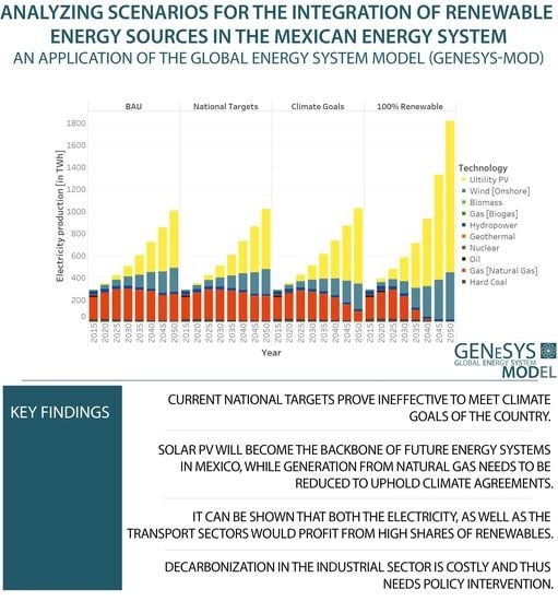
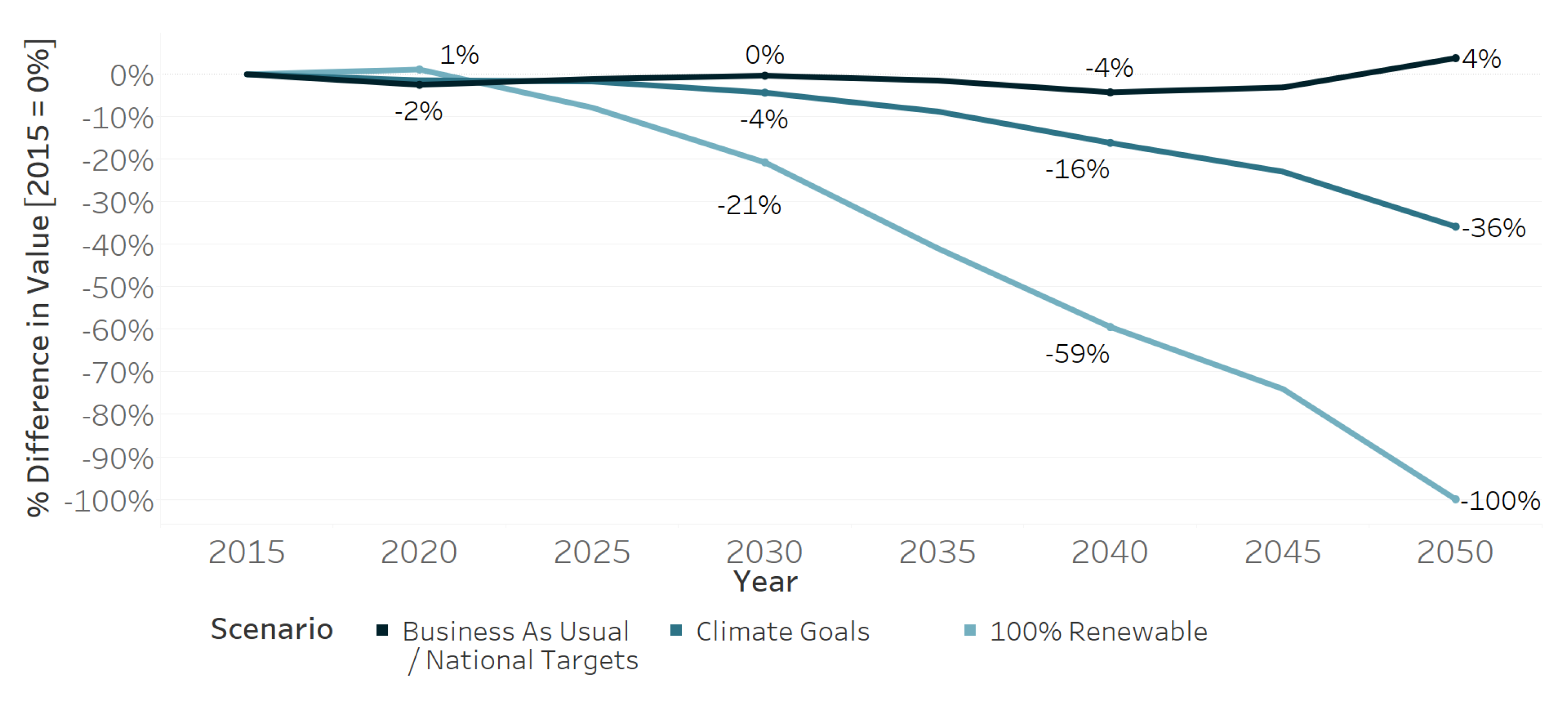
The primary objective of this optimization study is to answer four questions: first, how do costs and power mixes change in response to variations in energy and climate policies? Specifically, what are the effects of current renewable targets and climate goals vis-a-vis a scenario without the implementation of climate policies and another attaining full decarbonization. Second, what is the 2050 cost-optimal share of renewables in the Mexican energy mix for the power, heating and transportation sectors? Third, what is the marginal cost increase in each sector resulting from deviating from cost-optimal renewable targets? And fourth, are the climate goals and renewable targets aligned and how much do these deviate from the full decarbonization and policy free scenarios? To answer these questions we use four different scenarios —BAU, National Targets, Climate Goals and 100 percent Renewables—plus a iterative optimization routine of the Mexican energy system. We answer the first question by comparing all four scenarios, allowing us to contrast current public policies for the introduction of renewables or the reduction of emissions with the two additional scenarios (BAU, and 100 percent Renewables). To answer the second and third questions, we use an iterative optimization routine consisting of 20 different scenarios under increasing and binding renewable targets. In each optimization, the share of renewables in the system increases from 0% to 100% in 5% intervals. After each optimization, we calculate total discounted system costs and, with this information, determine the cost-optimal share of renewables in the energy system and the marginal cost of deviating from this optimal share. Finally, to answer the last question, we compare the effect of current National Targets and Climate Goals between them and with BAU in order to infer the alignment between both goals and their specific effect in the system. This article is, to the best of our knowledge, the first techno-economic model looking at the optimal cost-share of renewable technologies and the associated costs of deviating from this optimal in the transportation, heating and power sectors while accounting for sector coupling.
The following list presents a detailed explanation of the four main scenarios and the iterative routine:
  • BAU: the model has no requirements regarding renewable targets or climate goals.
  • National Targets: the model has to comply with current renewable targets in the power sector: 25% by 2018, 35% by 2024 and 50% by 2050 (Mexico defines these targets for clean energies (including nuclear as well as carbon capture and storage facilities). However, to stay in line with international comparisons, this paper defines clean energies as only those related to traditional renewable technologies.) [15]. Additionally, Renewable targets are only set for the power sector and all Mexican states should jointly achieve them. This cooperation means that renewable-rich regions can export their renewably produced surplus to other parts of Mexico.
  • Climate Goals: the model has to comply with current climate goals for the reduction of GHG emissions: 30% by 2020 and 50% by 2050 [16]. The climate objectives are defined on the national level across all sectors and regions of the economy. The model minimizes costs across all sectors with the underlying goal of achieving the necessary reductions in greenhouse gas emissions.
  • 100 percent Renewables: the model has to reach full decarbonization of the energy system by 2050.
  • Iterative routine: The model runs 20 different optimization routines by assuming 20 different renewable shares. The share of renewables in the system starts at 0% and linearly increases in 5% intervals until it reaches 100%. At each iteration, the model is required to comply with the renewable share without exceeding it.
Analyzing the Mexican energy system is interesting for several reasons. First, Mexico is one of the largest greenhouse gas emitters (13th) [17], oil producers (11th), electricity producers (13th), electricity consumers (15th), natural gas consumers (9th) and oil consumers (10th) in the world [18]. Second, the country has a high potential for the deployment of renewable technologies, like solar and wind, with respective potential capacities of 1172 and 583 gigawatts [19]. Third, the geographical location of the country opens the possibility of further integrating its electricity system with the United States and Canada, forming an integrated North American energy market, which would be one of the largest in the world.
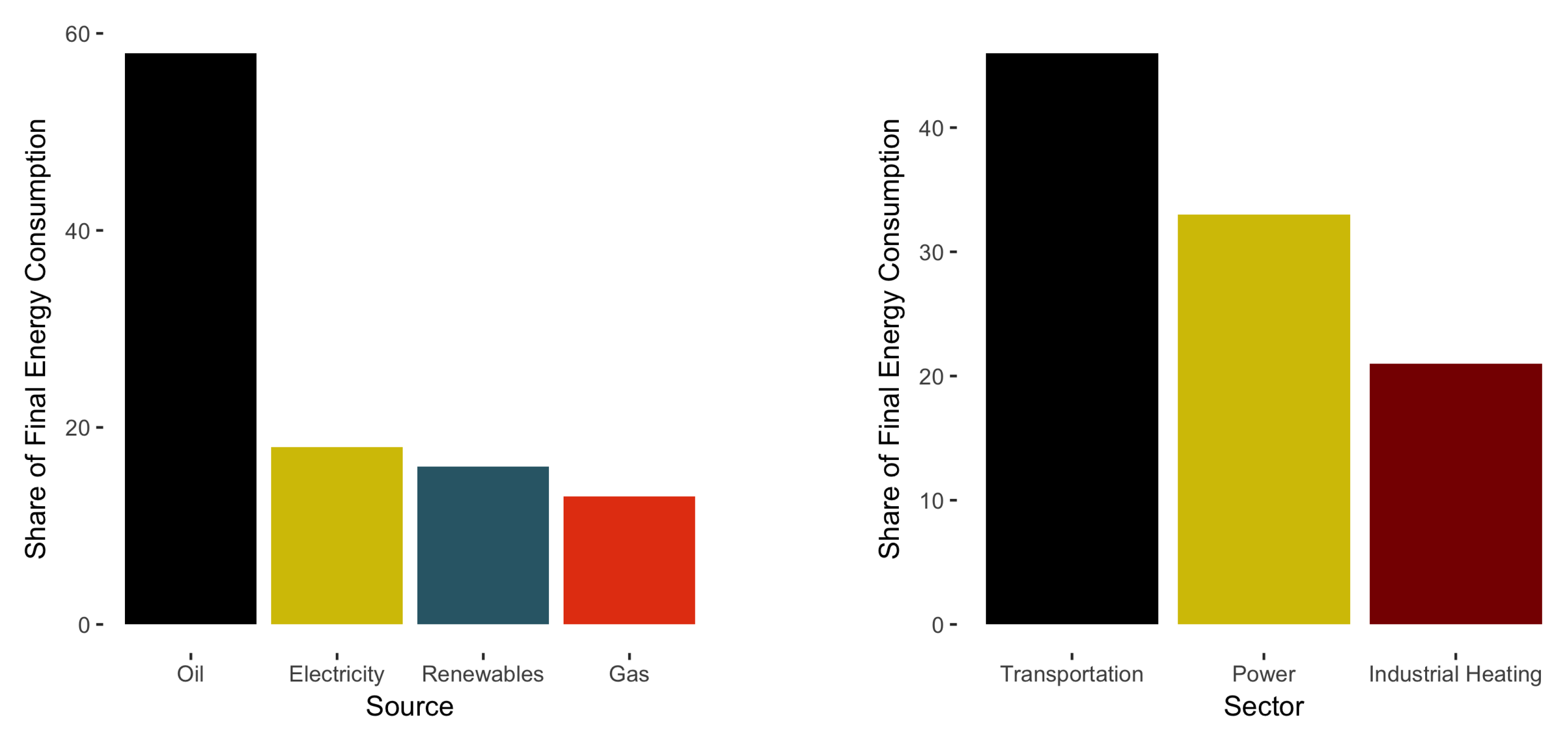
Currently, the Mexican energy mix is heavily reliant on fossil fuels. Figure 1 (left) plots the input share of each energy carrier in the mix. As can be seen, the system heavily relies on oil to satisfy its energy demands. Regarding the sectoral composition of the energy system, Figure 1 (right) illustrates that the transportation sector is responsible for the highest share of demand for energy in the country.
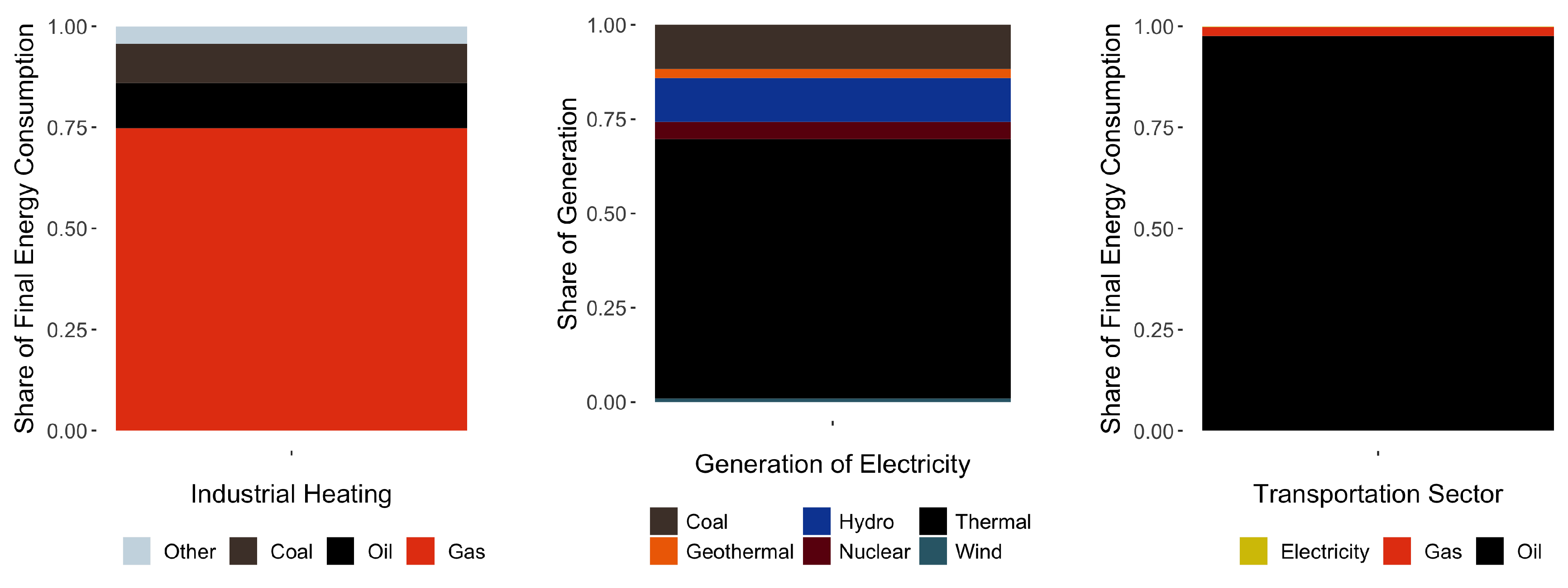
Figure 2 plots the fuel and technology mix of the demand for energy in each sector. Industrial heating heavily relies on natural gas, transportation on oil and the generation of electricity on thermometric, carboelectric and hydroelectric power plants. Specifically, natural gas has increased its share in the energy mix because of steady increments in the national demand for electric power and drops in the price of natural gas due to fracking activities in the United States (see Wang et al. [20]) that push oil away from the energy demand in the power and heating sectors. In 2002, natural gas was responsible for 37% of national capacity and 46% of electricity generation. By 2015 these shares had grown to 49% and 53% respectively. In general, 81% of all required new capacity between 2002 and 2015 came from natural gas power plants.
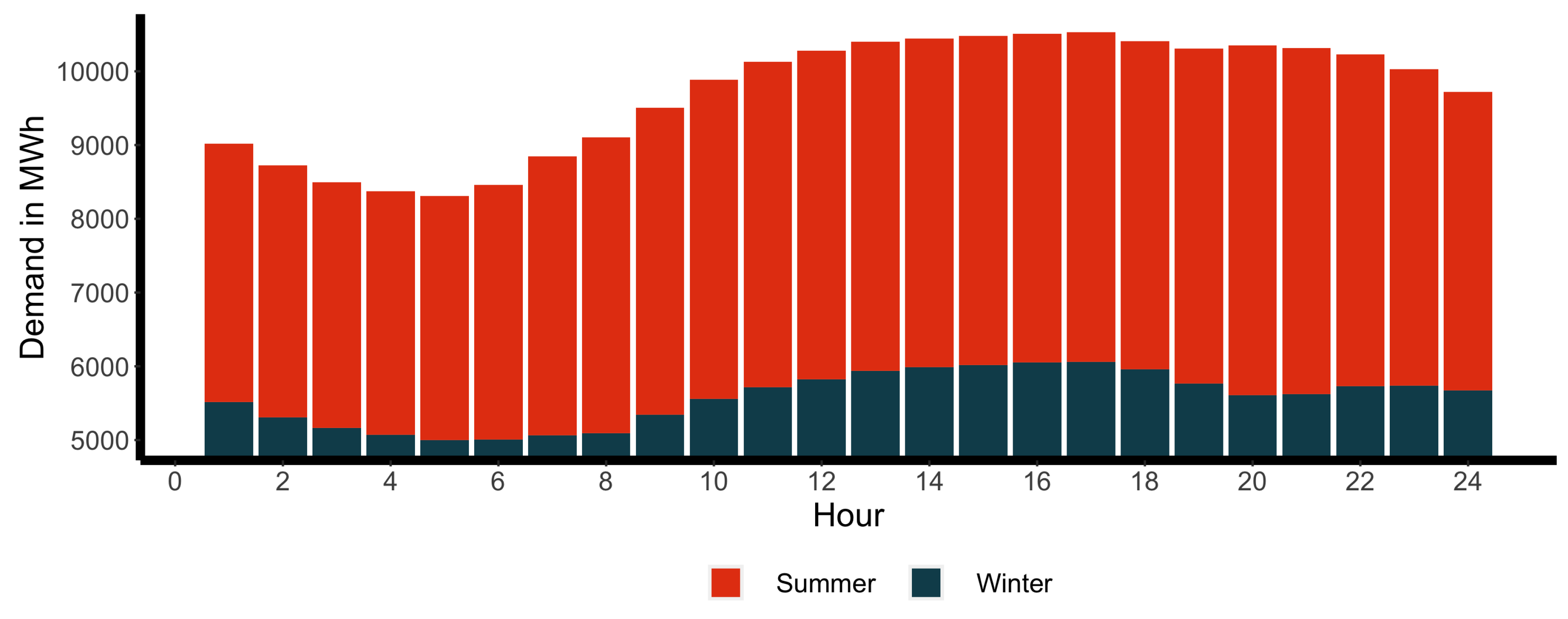
In 2015, the country consumed 288,232 GWh of electric power. It reached minimum demand on 1 January, at 18,341 MWh/h and maximum on 14 August, at 39,840 MWh/h. Higher demand for electric power comes in the summer months and afternoons due to the use of air conditioning and cooling technologies. This peak demand coincides with periods of high solar radiation when photovoltaic facilities can produce more power but is counter-cyclical to the production of wind and hydroelectric technologies. Figure 3 plots the intraday behaviour (load curve) of the national electric system for an average winter and summer day.
The industrial heating sector (the heating sector consists of residential and industrial heating. However, due to its geographical location, Mexico has no relevant demand for house heating) has no available public information on its energy demand. However, data on total energy and electricity demand at the industry level is publicly available [21]. Using this information, under the assumption that industrial demand for energy comprises electricity and heating and then combining it with the gross domestic product estimates of each industry at the state level [22], allows us to create an approximated value for the demand for heat in each control region. Imputed values show an aggregated heating demand in 2015 of 1060 Petajoules (PJ). The industries contributing most to this share are steel, cement and chemical at 18%, 12% and 13%, respectively.
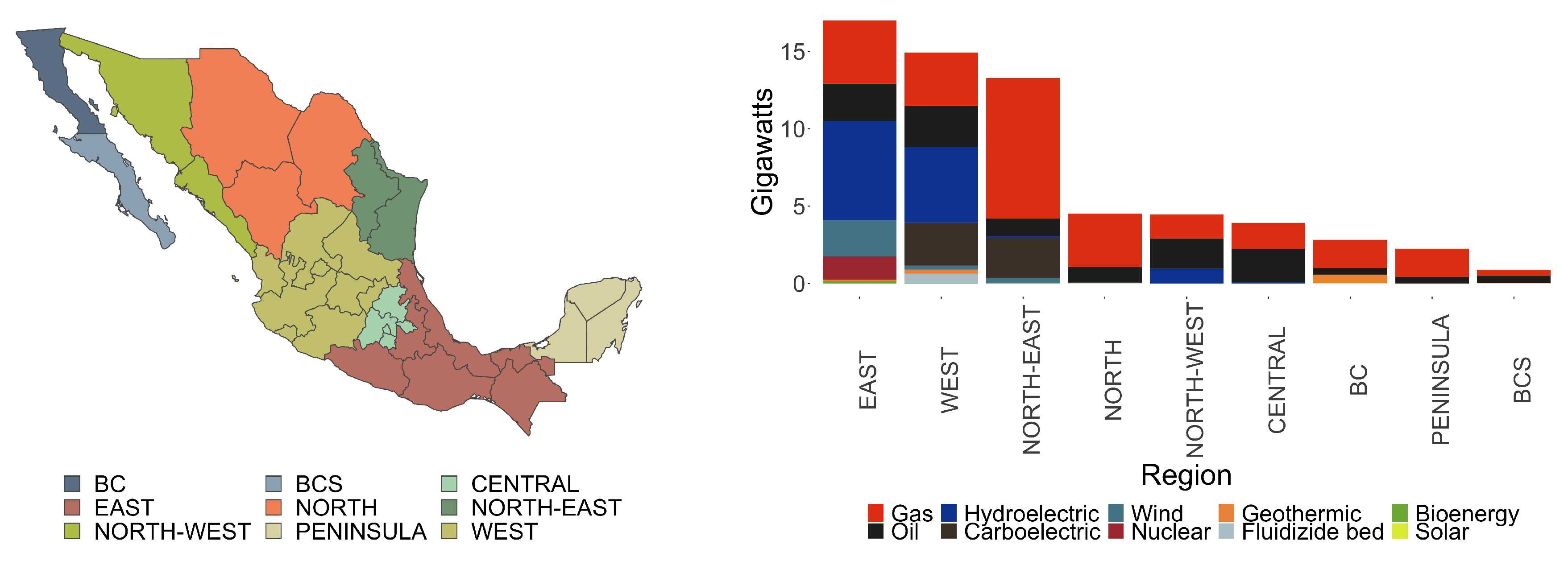
The national center for energy control (CENACE) divides the country into nine different regions. The model uses these regions to optimize the Mexican energy system. However, the regions of the model are slightly different than the regions of CENACE as the datasets with energy information come at the state level and the regions of CENACE are defined at the municipality level. Figure 4 maps each region into the map of Mexico and plots their respective installed capacity (for more information about the regional disaggregation, see Appendix A).
The rest of this article is structured as follows: Section 2 describes the data sources. Section 3 provides a historical review of numerical models in energy markets, explains the structure and characteristics of GENeSYS-MOD and outlines some related literature. Section 4 presents the results of the model and Section 5 concludes, summarizing the main findings.

2. Data

Numerical models of energy systems require large quantities of information on the electric, transportation and heating sectors to provide accurate estimates on the behaviour of the whole energy sector. For the Mexican power sector, capacity and generation data come from the Energy Information System of the energy ministry [21] and the North American Cooperation on Energy Information System [23]. Data on the potential for renewable sources is taken from the National Atlas for the Assessment of Areas with High Renewable Potential [19] and the National Inventory of Clean Energies of the Energy Ministry [24]. Load profiles per state, nodal structure and transmission capacities come from citizen requests to the National Center for Energy Control. Finally, planned mid-term improvements to the transmission grid originate from the National Electric System Development Program 2017 [25].
Transportation data on the number of cars, buses, trains, passengers and cargo, as well as the length of highways, railways and motorways and total energy consumption was obtained from the Ministry of Transportation and Communications statistics portal [26].
For industrial heating, unfortunately, there is no publicly available data on the exact demand in each region. However, we impute the regional demand with the following method. We assume that national consumed energy by the industrial sector ( δ s t ) is the sum of electricity ( ϕ s t ) and heat consumption ( γ s t ): δ s t = ϕ s t + γ s t . (The data on energy and electricity consumption may disregard production or transportation losses. Unfortunately, there is no available information on the accountability process with which the government reached these figures. To determine the demand of industrial heat in each state we thus assume the following. All three: total consumed energy, power and heat are subject to a losses of the form δ s t δ s t ^ = ( ϕ s t ϕ s t ^ ) + ( γ s t γ s t ^ ) , where the hat above the variable indicates the aggregate of transmission, production and efficiency losses. By a simple exercise, we can see that δ s t = ϕ s t + γ s t ( ϕ s t ^ + γ s t ^ δ s t ^ ) which can be simplified to δ s t = ϕ s t + γ s t + ϵ s t . The main assumption of this estimation is that ϵ s t 0 or equivalently ϕ s t ^ + γ s t ^ = δ s t ^ .) The national system of energy information provides national data on the first two elements: industrial consumed energy and electricity. This information allows us to determine the national demand for industrial heat. Once we obtain the national demand for industrial heat, we use additional segregated national data on national energy and power demand per industry to determine the share of the national heating demand that accrues to each industrial sector. Then we use data from the 2015 economic census of the national institute of geography and statistics (INEGI) to calculate the share of each industry in each state and, thus, the demand for heat that accrues to each state. For example, if the national heating demand of the cement industry is 6.816 PJ and if 50% of the national gross domestic product of the cement industry belongs to a specific state, this state will also have 50% of the total demand (3.408 PJ). Concerning additional inputs, Table 1 summarizes the main sources and assumptions. Fore additional input data, please refer to Appendix B.

3. Model

Numerical models of energy systems use a system of equations to simulate the consequences that exogenous shocks and different states of the world have on the overall structure of the energy sector. The necessity for this kind of model originated in the acute effects experienced by oil-dependent industrialized countries during the 1970s oil crisis. The oil crisis increased the necessity to simulate the behaviour and reliability of energy markets under exogenous supply and demand shocks [35]. After the development of these oil models, there was a steady change in scope to incorporate climate change, pollution and other relevant externalities from the energy sector. Traditionally, these new energy models analyze the interdependencies and optimal shares between the three main sources of primary energy: fossil fuels, nuclear and renewables. However, recent debates regarding the possibility of fully decarbonized energy systems (Clack et al. [36], Jacobson et al. [37], Hansen et al. [38], Geels et al. [39]) and the availability of low-cost storage technologies shifted interest to the analysis of decarbonization paths and the future development of green energy operations.
Overall, numerical models can be broadly divided into techno-economic and macroeconomic models [35]. Techno-economic models permit separating the energy system into different technologies, processes and interdependencies across energy carriers. This ability to divide the energy system into smaller technology blocks allows the model to internalize the impact of specific policies in each subdivision and to play with the relationships between sectors, technologies and regions. Macroeconomic models, on the other hand, account for the economic determinants behind energy systems. They experience a trade-off between technical detail and economic insights while attempting to capture links between the energy sector, the economy and society. The separation between techno-economic and macroeconomic models resulted in the need to develop a new set of models that internalize the advantage of both approaches. For example, computable general equilibrium (CGE) models simulate energy systems up to a certain level of technical detail within a particular market structure. Prominent examples of CGE models are the MIT-EPPA model used to simulate the world economy and the GEM-E3 model used by the European Commission [40]. Concerning other prominent techno-economic models. One well known model is the MARKAL model, developed by the International Energy Agency [41]. While MARKAL belongs to the group of optimization models, recent modules try to bridge the gap between the techno-economic and macroeconomic models [42], one of them being TIMES (The Integrated MARKAL-EFOM System). TIMES combines a technical engineering with an economic approach, thus merging the characteristics of both [43]. Further, recent techno-economic models try to incorporate aspects of system dynamics into energy system models, for example, POLES [35,44]. System Dynamics models are used to analyze the behaviour of different actors and, thus, are able to provide new insights to energy system modelling.
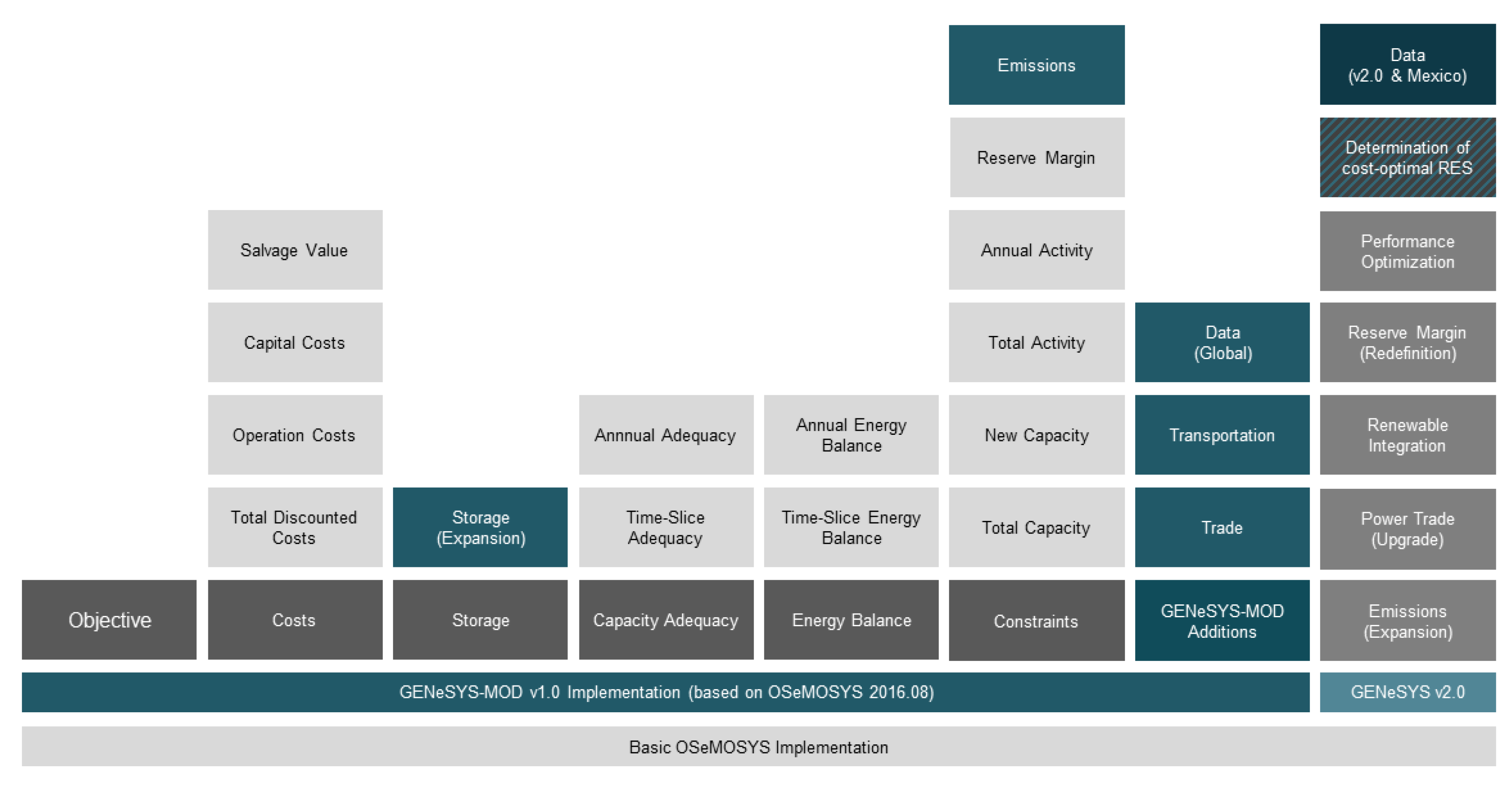
GENeSYS-MOD is based on the Open-Source Energy Modelling System (OSeMOSYS) framework, developed by the Royal Institute of Technology in Stockholm, Sweden [45]. OSeMOSYS was used by Moura et al. [46] in a game-theoretical framework to understand the bargaining power of South American countries concerning energy policies, by Rogan et al. [47] to analyze the impact of different energy efficiency measures in the Irish energy market and by Lyseng et al. [48] to model the Alberta, Canada, energy system and to study the ability of the region to comply with the 2 degrees commitment of the COP 21. Löffler et al. [14] extended OSeMOSYS to GENeSYS-MOD by including new functionalities, such as a modal split for transportation, an improved trade system and an enhanced focus on environmental budgets. Lawrenz et al. [49] further enhanced GENeSYS-MOD in their case study on transition pathways of the Indian energy system, while Burandt et al. [34] introduced the second model version, with improvements to storages, time slices and performance optimization (for a detailed description of GENeSYS-MOD and its blocks of functionality, see Appendix C).
Specifically, GENeSYS-MOD is different from CGE models because of its capacity to split the energy market into different sectors, technologies and processes; from traditional electricity market models because of its capacity to endogenously optimize the power, transportation and heating sectors, while accounting for sector coupling (Sector coupling refers to the interdependency and substitutability of energy carriers across sectors, for example, electric vehicles and electrolysis.); and from macroeconomic models because of its high level of technical detail. Overall, GENeSYS-MOD is similar to the TIMES model regarding its modular structure and general modelling paradigm. The key advantage of GENeSYS-MOD is the open-source approach of code and data and that the model is freely available. The capacity of GENeSYS-MOD to subdivide the energy system into sectors, technologies and regions; its ability to account for sector coupling; and its high degree of technological features are necessary characteristics of a model attempting to understand the consequences of exogenous variations in energy and climate policies on each supply option, energy sector and modeled region. Overall, numerical models allow analyzing a great variety of problems across several sectors and sciences. Techno-economic models have shown the ability to analyze costs and effects of a transition toward low-carbon technologies in national energy and power mixes. The power sector is the one sector that historically and recently, has received the most attention. With European [50,51], American [52] and global models [14,53] analyzing different transition pathways and their effect on the aggregated cost of the system. Additionally, the scope of these models have expanded to other regions, like China [54] and India [49,55], as well as to other sectors of the energy system in multi-sectoral models [33]. The latter is of high importance, as most previous studies only target the power sector, omitting significant effects due to sector-coupling. Still, a detailed analysis of the Mexican energy system using an integrated, multi-sectoral, approach is missing.
GENeSYS-MOD optimizes the energy system by using a system of linear equations as constraints and inputs to minimize the aggregated cost of the energy system, while securing the supply of energy in a specific region. Equations (1) and (2) show the objective function, as well as the decomposition of technology costs in the model. Equation (1) minimizes the total discounted costs of the energy system (z). Furthermore, Equation (2) defines the costs of each technology as the discounted sum of operating costs, capital investment, emission penalties and salvage values. These equations serve as the core of the model, with additional constraints (see Appendix C) determining the proper functionality of elements, such as energy balances, emission limits or renewable integration.
Min z = y , r ( t T o t a l D i s c o u n t e d C o s t B y T e c h n o l o g y ( y , t , r ) + s T o t a l D i s c o u n t e d S t o r a g e C o s t ( y , s , r ) + D i s c o u n t e d A n n u a l T o t a l T r a d e C o s t s ( y , r ) + f , r r D i s c o u n t e d N e w T r a d e C a p a c i t y C o s t s ( y , f , r , r r )
T o t a l D i s c o u n t e d C o s t B y T e c h n o l o g y ( y , t , r ) = D i s c o u n t e d O p e r a t i n g C o s t ( y , t , r ) + D i s c o u n t e d C a p i t a l I n v e s t m e n t ( y , t , r ) + D i s c o u n t e d T e c h n o l o g y E m i s s i o n s P e n a l t y ( y , t , r ) D i s c o u n t e d S a l v a g e V a l u e ( y , t , r ) y , t , r
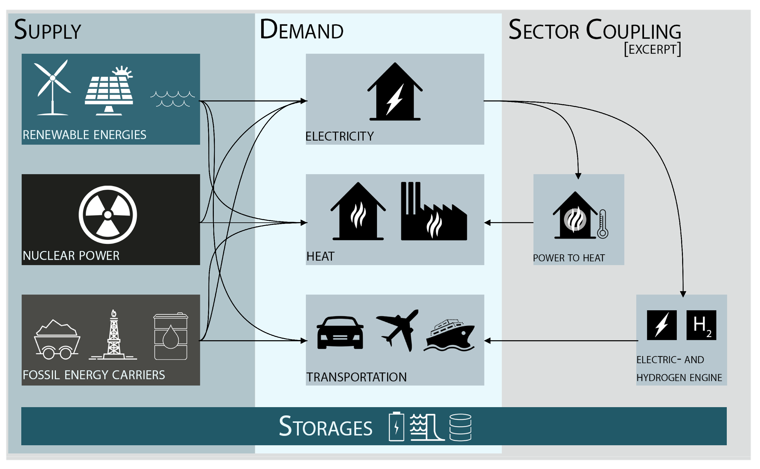
Figure 5 portrays a stylized version of the general structure of the model. From left to right, we have power generation technologies. These technologies provide electricity to the grid and extract resources from raw energy carriers that also provide energy for industrial and residential heating. The electricity provided to the power grid can be used to satisfy power demand in the region, regional power trade, electric engines, batteries and generation of gas or heat through power-to-heat and power-to-gas technologies. Other critical energy carriers are waste and biomass, which can be used for biofuels or direct use for heat. Finally, the transportation sector is divided into passenger and freight transport with respective technology options. The model then uses the range of technology options to fulfil the (exogenously) defined demands for electricity, heat and transportation, while staying true to constraints, such as renewable targets or emission reduction goals. To achieve this, the model optimizes the construction of new capacities of generation facilities, sector-coupling options, and energy storage. (Since the model can choose freely how to fulfil the final demands, it can use technologies that link the different sectors, usually by electrification. This means that heat or transportation can be provided by electric options, thus coupling the traditionally segregated sectors). As a result, the cost-optimal pathway toward the achievement of these long-term scenarios is obtained for all sectors. For more information on the technical side of the model, please refer to Appendix C, Löffler et al. [14], Howells et al. [45] and Burandt et al. [34].
As a techno-economic numerical model, GENeSYS-MOD is subject to the relevant limitations of these kind of models. It requires exogenous inputs on forecasted demands, costs and technological paths. Regarding the demand for transportation, power and heating, these come from third-party sources, such as the national program for the development of the energy system (PRODESEN) or are imputed with the use of GDP and population estimates. Furthermore, because of the integrated modelling approach for the entire period between 2015 and 2050, it is only possible to include a given number of time slices per year, sixteen-time slices, including four different seasons (spring, summer, autumn, winter) and four intraday cuts (morning, peak, evening, night). These time slices intend to account for peak demand periods in summer and afternoons. Welsch et al. [56] compare an enhanced OSeMOSYS implementation with 16 time slices to a full hourly dispatch model and find the differences to be relatively small (roughly 5% deviation). However, it is true that more granular time windows would be optimal, given the difficulties to push the system toward a full decarbonization path. Linking the more broadly-based energy system development done in this paper to more detailed electricity sector models might be a good point for further research. Further, assessing the cost-optimal transition on a smaller regional level (e.g., municipalities) can lead to additional insight into the development of the Mexican energy system. This also holds true for the assessment of optimal renewable shares, where a regional approach (instead of a sectoral approach) might provide further insights, especially since policies are often determined at a regional level (e.g., using decision making processes, instead of pure optimization) [57,58,59]. Finally, capital, variable and O&M costs come from exogenous sources and, therefore, influence the model results.
For this exercise, the model looks at the Mexican energy system by dividing it into three sectors (power, (low-and high-temperature) heat and (passenger and freight) transportation), 9 regions (BCN, BCS, North, Northeast, Northwest, West, Central, East and Peninsula), a multitude of generation technologies (e.g., utility PV, onshore wind, hydropower, biomass, gas (biogas), geothermal, nuclear, oil, gas (natural gas), hard coal, ...) and 16 time-slices. The modeled period runs from 2015 to 2050, computed in 5-year steps, with 2015 serving as the baseline (calibrated based on the data outlined in Section 2).

4. Results

Before addressing the results of each scenario run, it is essential to point out that there were no noteworthy differences between BAU and National Targets, as shown in Figure 6. The objectives of renewables penetration in the power sector of National Targets are attained even without the intervention of climate policies. This outcome means that current national targets in the power sector are insufficient and do not shape the behaviour of the market. Because the results from both scenarios are so similar, the remaining section presents them as a unified scenario: BAU/National Targets. To verify the proper workings of the model, a model validation has been conducted and can be found in Appendix D.

4.1. Electricity Sector

The electricity sector sees a significant increase in generation from of renewable technologies. This general trend is independent of the scenario (see Figure 6 and Figure 7). However, the Climate Goals and 100 percent Renewables scenarios result in overall higher renewable shares. Solar power reveals itself as the dominant technology in all scenarios. Even in the BAU/National Targets scenario, it reaches 52.3% of electricity generation, while for 100 percent Renewables, it provides as much as 75.4% by 2050. Electricity generation due to sector-coupling drastically reacts to more ambitious climate targets, with the 100 percent Renewables scenario clearly surpassing BAU/National Targets, as well as Climate Goals (see Figure 6 and Figure 7). In the BAU/National Targets scenario, generation from natural gas increases in the early years of the modelling horizon, peaking in 2030 and then remaining steady with just a small decline toward the end of the modeled period. For the other two scenarios, it peaks in 2025, after which generation from gas-fueled technologies immediately starts to decline. In 100 percent Renewables, the production from natural gas facilities almost disappears by 2040.
Each regional power mix heavily depends on its environmental endowments and demand structure. Figure 8 exhibits the regional development of electricity generation for each scenario. While the system is strongly reliant on natural gas across all scenarios for the year 2030, renewable generation also starts ramping up. Solar technologies are ubiquitous to Mexico and appear with varying intensities across all regions. Hydroelectric power generation remains relatively constant (in absolute terms), although its share diminishes due to the general increase in electricity generation. By 2050, all scenarios show large amounts of solar PV, especially in the Northern regions. Especially in the 100 percent Renewables scenario, the North region supplies large amounts of solar-based electricity to the surrounding regions. Finally, biofuels only appear competitive in the electricity sector for the Central region in the scenarios Climate Goals and, to a lesser extent, in 100 percent Renewables. This is due to the region’s small size and comparatively small endowments of RES potentials, yet high energy demands.
Table 2 presents the installed capacity for natural gas, onshore wind, solar PV and storage technologies across years and scenarios. Intense solar radiation across the nation drives the steady increase in solar PV deployment, with 2050 values ranging from 320.73 GW (BAU/National Targets) to 842.89 GW (100 percent Renewables). Wind also experiences a steady expansion of generation capacities (especially in the East region) but to a much smaller degree than solar. Onshore wind capacities increase from 3.4 GW in 2015 to 56.9 GW in BAU/National Targets, 67.8 GW in Climate Goals and 121.5 GW in 100 percent Renewables by 2050. Strong sector-coupling effects between the electricity and other sectors (see Section 4.2 for more cross-sectoral information) drive the exponential growth behind wind and solar power in the 100 percent Renewables and Climate Goals scenarios. Furthermore, going hand-in-hand with generation from intermittent renewables, the need for electricity storage also increases. While BAU/National Targets utilizes about 110.1 GW of electric storage options, (electricity storage in GENeSYS-MOD v2.0 include Lithium-Ion Batteries, Redox-Flow Batteries, Pumped Hydro Storages and Compressed Air Electric Storages) the 100 percent Renewables scenario requires about 366.7 GW. This difference in storage capacities implies that the storage requirements of 100 percent Renewables are more than three times higher than in BAU/National Targets.

4.2. Energy System Development

Looking at the entire energy system, RES play a vastly different role for each scenario (see Figure 9). While the most ambitious 100 percent Renewables scenario sets the target of 100% renewables use in 2050 (and thus is required to achieve it), the more conservative BAU/National Targets does not enforce climate targets and, thus, remains significantly fueled by conventional energy sources, namely natural gas and oil, even as late as 2050. The Climate Goals scenario takes the middle ground, with about 50% RES-based energy generation by 2050. The total final energy generation only shifts marginally between the scenarios but with Climate Goals and 100 percent Renewables consistently lower than BAU/National Targets. This is due to efficiency gains made possible by sector-coupling, with electrification options being used far more extensively.

4.2.1. Sectoral Analysis

Figure 10 plots the sectoral share of RES across scenarios. The figure also portrays (sector-coupling) electricity usage in the sectors mobility (aggregating passenger and freight transport) and industrial heating.
For the power sector, the entrance of solar and wind technologies to the power matrix replaces natural gas across scenarios. The only difference between them is the steepness of the decarbonization path. The electricity sector of 100 percent Renewables is fully decarbonized by 2045, while Climate Goals still has a marginal share of natural gas facilities in 2050 and under the BAU/National Targets, natural gas production remains at almost 30%. After the power sector, the transportation sector is the next to decarbonize. The sector remains oil-powered in the BAU/National Targets scenario, although a significant share of electricity and RES appears after 2025. For Climate Goals, the transportation sector is about 80% decarbonized by 2050, mostly with the use of electric vehicles and biofuels. 100 percent Renewables achieves 100% renewables in the transportation sector with a higher share of electric-powered vehicles. On the other hand, a particular issue in the path toward full decarbonization is high-temperature heating. In high-temperature heating, both BAU/National Targets and Climate Goals show almost no decarbonization, only 100 percent Renewables enforces a renewable target that obliges the total decarbonization of industrial heating. When the model decarbonizes industrial heating, it opts for a mixture of electricity, hydrogen and biomass (mostly in the form of biogas). The reason behind difficulties in the decarbonization of industrial heating is the sharp cost difference between low-carbon and (regular) carbon-intensive processes in the sector.
In general, a strong trend of sector-coupling can be seen when climate goals are prioritized. This holds mostly true for the mobility sector, where even the BAU/National Targets scenario achieves about 30% electricity share, reaching almost 90% in the 100 percent Renewables scenario. This behaviour also explains the heavy increase in electricity generation across scenarios, as observed in Section 4.1.

4.2.2. Costs

In this section, we analyze the effect of the iterative routine. This routine consists of optimizing the power, transportation and industrial heating sectors under 20 different and binding shares of renewables. The binding shares start at 0% and grow in 5% intervals until reaching full decarbonization. Figure 11 presents the sectoral percentage change in total-discounted-system-costs between a fully decarbonized system and a partially decarbonized one. This graph does not portray any specific scenario assumption but instead takes the technology learning curves and forces the model to use a fixed percentage of renewables in each respective sector(s). Electricity used in the heat or transportation sectors is being distributed to renewable/non-renewable energy via the annual share of RES in the power mix (e.g., RES produced 70% of electricity in 2035, then 70% of electricity in transport would count as renewable and 30% as non-renewable). In the figure, values above zero represent higher total costs than the 100 percent Renewables scenario, while values below zero mean that this level of RES integration would be more cost-competitive than 100 percent Renewables. Naturally, the minimum of the curves represents the cost-optimum share in each of the sectors. To the best of our knowledge, this is the first time a techno-economic optimization model looks at cost variations of the entire energy system across different shares of renewables while accounting for sector coupling.
For the power sector and the energy system as a whole, the model portrays two U-shape convex curves. Industrial heating resembles a curve of positive slope, with the percentage increase in total system costs steadily increasing with the share of renewables. On the other hand, the transportation sector display the opposite behaviour, with a negative slope indicating that sector costs decrease with renewable integration. Two insights come from this figure. First, the energy-system cost-curve reaches its cost-optimal share at 75%. High-temperature heat reaches it at 5%, power at 75% and transportation at 90%. Another result is the low-cost difference between the cost-optimal point of 75% RES in the electricity sector and its marginal cost of increasing its share of renewables. Between 75% and 100%, the cost difference is merely 1.28%. For the entire energy system, this difference increases to 6.09% of total system costs due to the high costs of decarbonizing industrial heating. It is worth mentioning that uncertain technology learning curves, fossil fuel prices or energy demands drive these results. However, these results provide an estimate of the cost difference between different penetration scenarios of renewable sources in the energy sector.
A sensitivity exercise, introducing an exogenous CO2 price, representing an internalization of adverse external effects of carbon dioxide emissions [60], is shown on the right-hand side of Figure 11. The introduction of such an environmental carbon tax (of 180€/tCO2 in 2015) shifts results quite significantly, although the overall picture remains the same. Industrial heat still sees a low share of RES in its cost-optimal version, while the electricity sector moves up to 95%, pushing the cost-optimal share of RES in the energy system to 85%. In addition, the steepness of the curves is shifted, with a vastly higher increase in total system costs for low amounts of renewables. This exercise demonstrates that a CO2 tax that internalizes these negative environmental effects can have a significant effect on the outcome of such cost-driven studies and move the cost-optimality even further in favour of RES.

4.2.3. Emissions

Figure 12 plots the relative annual emissions for each of the three scenarios compared to 2015. While the Climate Goals scenario reduces its emissions by 36%, the BAU/National Targets scenarios remain rather constant in their emissions and result in a net increase of about 4% in 2050. What is important to keep in mind, however, is that this 4% increase in emissions in BAU/National Targets goes against a major increase in energy demand across all sectors that comes along with the expected growth of population and wealth. Finally, 100 percent Renewables reaches its target of 100% decarbonization in 2050.
Summing up the yearly emissions, 100 percent Renewables, with its 100% renewable target in 2050, reaches total emissions of about 7.16 Gt CO2, while Climate Goals emits about 9.63 Gt CO2 and BAU/National Targets just above 12.0 Gt CO2, thus more than 60% more than the 100 percent Renewables scenario.

5. Conclusions

In this article, we use the Global Energy System Model (GENeSYS-MOD) to optimize pathways for the Mexican energy system under different energy and climate policies. GENeSYS-MOD is a techno-economic cost-minimizing energy model that differentiates from traditional bottom-up models by the integration of traditionally segregated energy sectors (power, transport and heat). The goal of the study is to analyze the consequences of current renewable targets and climate goals in the future cost composition and structure of the energy sector, to do this we use four different scenarios: BAU, National Targets, Climate Goals and 100 percent Renewables. BAU optimizes the energy system without any constraints regarding renewable targets or climate goals. National Targets forces the model to attain current renewable targets. Climate Goals does the analogous with Mexico’s climate goals, and, finally, 100 percent Renewables forces the optimization routine to decarbonize the energy system by 2050. Additionally, we also run an iterative optimization routine by increasing the share of renewables in each sector between 0% and 100% in 5% steps. In each iteration, the model attains, without exceeding, the imposed share of renewable sources. Our modelling approach allows us to investigate the cost consequences and changes in energy mix of national renewable targets and climate goals between the scenarios. Moreover, comparing BAU with Climate Goals and National Targets permits us to infer the suitability of these policies by understanding how much they deviate from the two extreme scenarios (BAU and 100 percent Renewables). Finally, the optimization routine allows us to determine the cost-optimal share of renewables in the energy system and the marginal cost of deviating from this optimal share. To the best of our knowledge, this paper is the first optimization approach analyzing how the total discounted costs of the energy system vary under different sectoral renewable targets. Additional contributions relate to the analysis of the Mexican energy sector while accounting for sector coupling and the insights gained from the comparison of various scenarios.
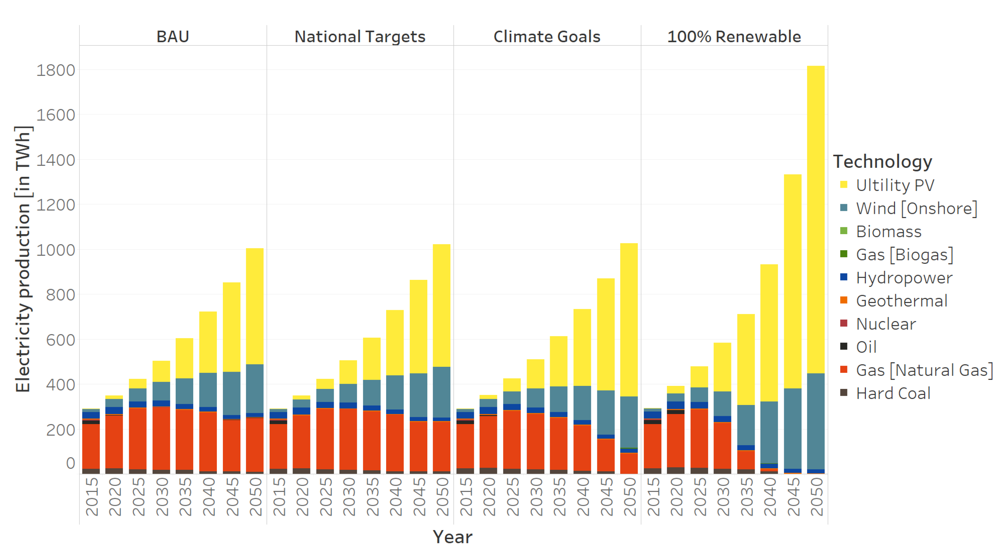
Results from the study show that Mexican renewable targets are insufficient and sub-optimal: the model shows that the optimal share of renewables for the generation of electricity is 80%, that is, 30% higher than current commitments in the national strategy for the promotion of clean fuels and technologies [
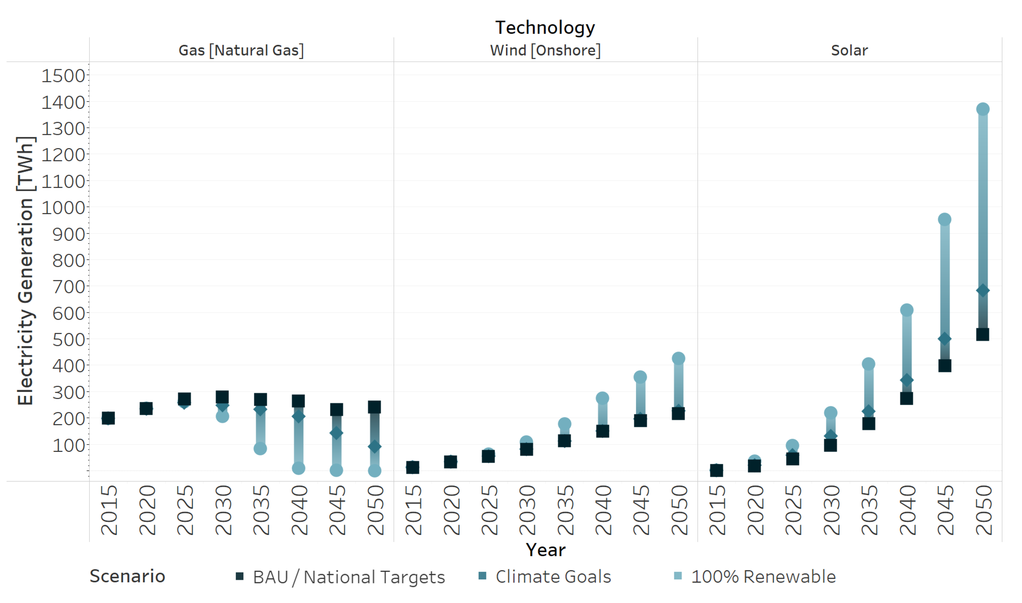
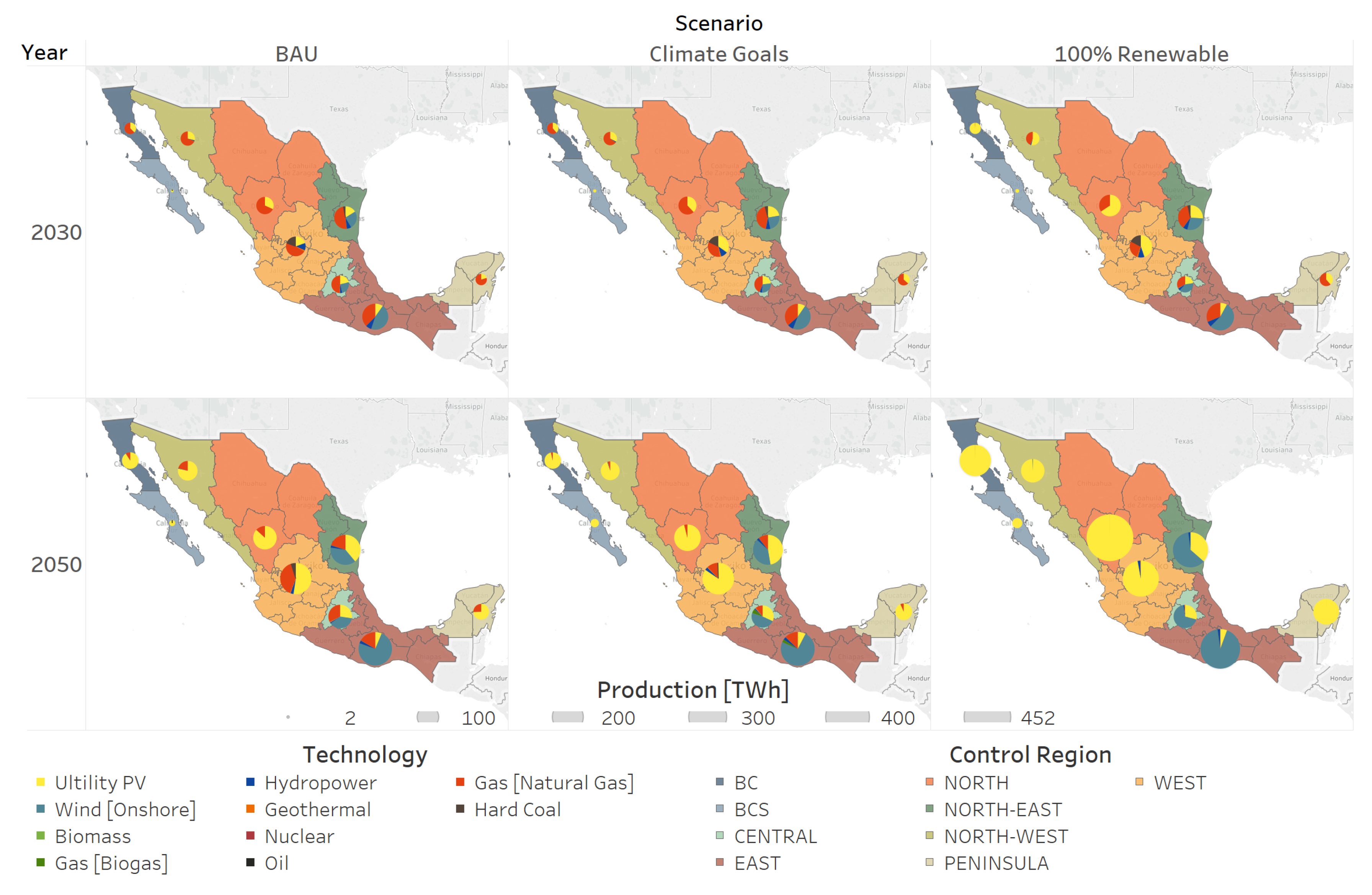
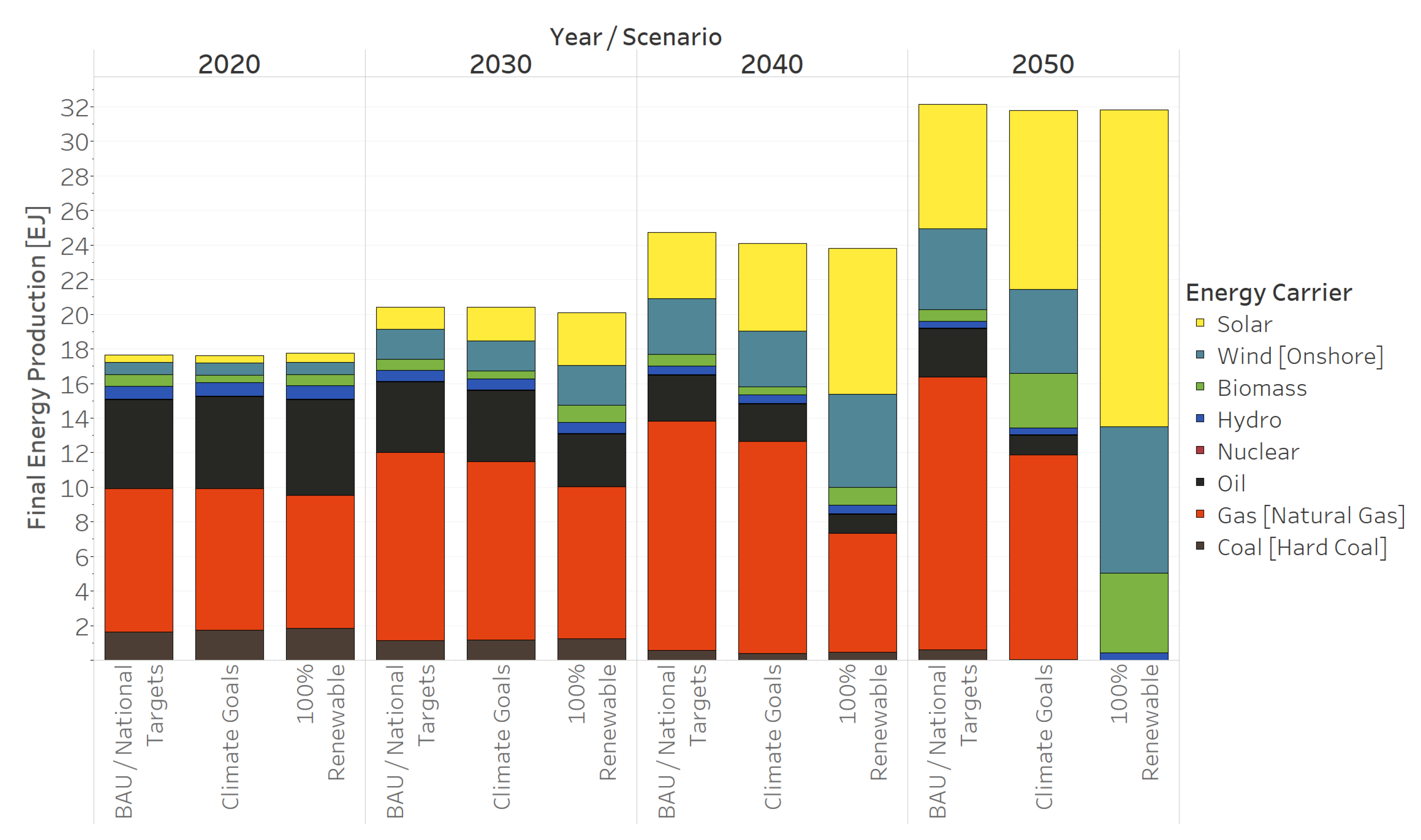
15]. Even more, the share of renewables in the power mix between BAU and National Targets is very similar. This indicates that current renewable targets do not even deviate from a scenario without climate policies, meaning that there is a misalignment between climate goals and renewable targets. In principle, both policies should aim for the same goal. For example, if the power sector renewable target of 50% is significantly lower than the penetration of renewables under the fulfillment of climate goals, it is redundant and inefficient to implement both policies. At the minimum, renewable targets should mimic the sectoral decarbonization paths of climate goals. Regarding the energy mix, natural gas and photovoltaics shape the future of the Mexican energy system, across all regions, except for the wind-rich East region, strongly relying on onshore wind turbnies for the generation of electric power. In the intermediate term, however, an ongoing dependence on natural gas can be observed across all scenarios. When aiming for full decarbonization (100 percent Renewables), the energy mix relies on solar, wind and biomass to satisfy the energy needs of the country, using the grid, as well as energy storages, as load balancing options.
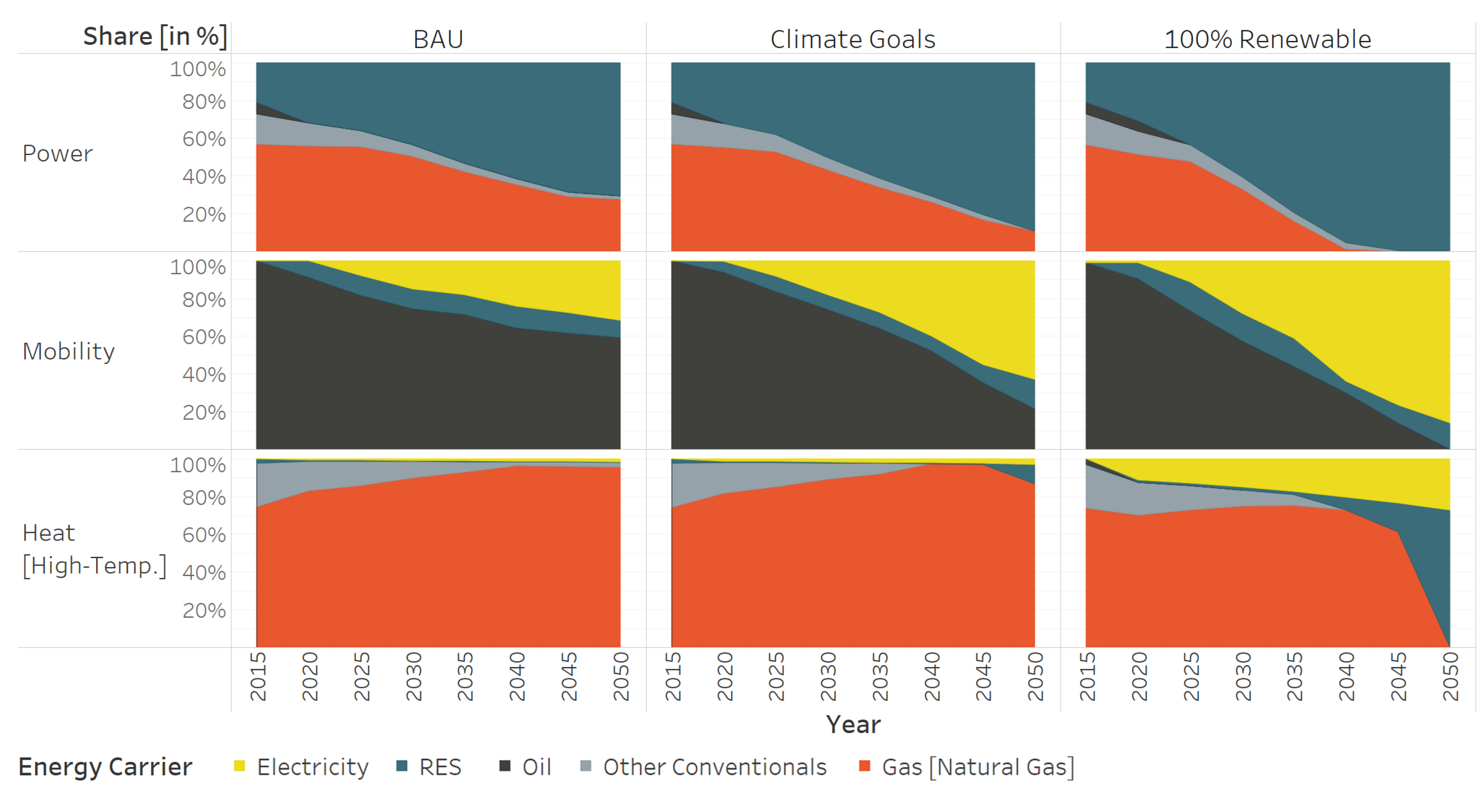
Concerning sectoral decarbonization paths, it is evident that the power, transport and heating sectors present different patterns. For electric power, the cost competitiveness of photovoltaics and wind turbines push the sector toward decarbonization across all scenarios and regions. Moreover, due to sector coupling, the introduction of these cost-competitive technologies in the power mix is a crucial factor for the decarbonization of the transportation sector. The higher the share of renewables in the power sector, the greater the introduction of electric vehicles in the transportation sector. The heating sector is the last sector to decarbonize because of substantial cost differences between conventional and renewable heat.
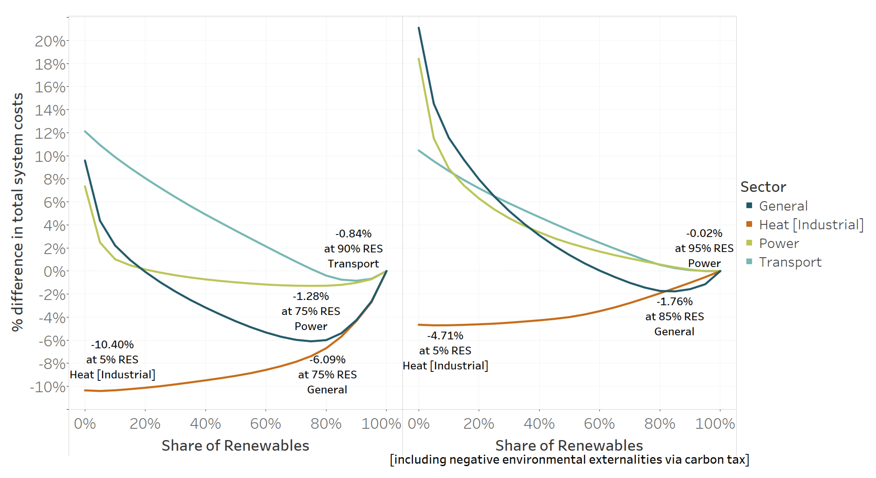
Furthermore, the computation of sectoral cost minima exhibits interesting results. As previously noted, the cost-optimal share of renewable targets in the power sector is 75%, 25% points higher than current renewable targets. For the transportation sector, the share is as high as 90%, suggesting significant economic advantages of increasing the share of electric vehicles in this sector. For the heat sector, its share reflects the high cost of renewable heat and present an optimal renewable target of only 5%. Finally, for the energy system as a whole, the 2050 optimal renewable share is 75%. As an additional exercise, we analyze how costly it is to increase the share of renewables in both the power and energy sectors. Increasing the power sector to full decarbonization only increases total costs by 1.28%; for the whole energy system, total costs would increase by 6.09% (mostly driven by industrial heating). Finally, the difference in total cumulative emissions between BAU/National Targets and 100% Renewable is 4.85 gigatonnes of C O 2 (more than 10 times the current yearly emissions of Mexico [61,62,63]).
The results of this study air several exciting conclusions: public policies for the introduction of renewables in the power sector need to change. They are equivalent to a scenario without climate policies, disconnected from the climate goals of the country and significantly lower than the estimated cost-optimal share of renewables in the power sector. Furthermore, aiming for more stringent shares of renewables in the power sector or stricter climate goals for the mitigation of greenhouse gases only marginally increases the total cost of the energy and power systems. Other relevant insights are the reliance of the power system on photovoltaic and natural gas, the high cost-optimal share of renewables in the transportation sector and its low counterpart in industrial heating. Moreover, this article can help policymakers in the design and implementation of specific targets and policies for the decarbonization of the heating and transportation sectors by providing the cost-optimal share of renewables in each sub-sector.

Author Contributions

Conceptualization, L.S., T.B., K.L. and P.-Y.O.; methodology, L.S., T.B. and K.L.; software, T.B. and K.L.; validation, L.S., T.B. and K.L; formal analysis, L.S. and P.-Y.O.; data curation, L.S., T.B. and K.L.; writing—original draft preparation, L.S., T.B., K.L. and P.-Y.O.; writing—review and editing, P.-Y.O. and K.L.; visualization, L.S. and K.L.; supervision, P.-Y.O.

Funding

This work was supported by the German Ministry for Education and Research (BMBF) under grant number 01LN1704A for the research group CoalExit.

Acknowledgments

Previous works of this research have been presented at various workshops and conferences in Mexico and across Europe. We therefore thank the conference and workshop audiences and in particular Christian von Hirschhausen, Claudia Kemfert, Juan Rosellon and Elmar Zozmann for useful discussions and suggestions, the usual disclaimer applies.

Conflicts of Interest

The authors declare no conflict of interest.

Appendix A. Regional Disaggregation

East, located in the eastern-southernmost part of the country has the largest installed capacity and penetration of renewables across regions. Wind-parks and hydroelectric-dams cover up to 50% of the region’s installed capacity. West, located in the center west of the country is the second largest region regarding installed capacity. Its energy mix has combined-cycle, hydroelectric, carboelectric and oil-indexed facilities as driving technologies. Northeast is located in the north-east of the country, next to the Gulf of Mexico and south of Texas. An extensive network of gas pipes connects it with the shale reserves of the United States making its power mix heavily dependant on natural gas. This region is also experiencing a surge of wind parks in the north part of the Gulf of Mexico. Northwest and North are industrial and scarcely populated regions that use combined natural gas, oil and dams to satisfy their energy demands. Central includes Mexico City and its metropolitan area plus additional center states. The region is poor in natural endowments and it is a net importer of electric power. Its power matrix consists of natural gas and oil. BC locates south of California, in the northwest of Mexico. It has natural gas and geothermal energy as the main sources of power. Finally, Peninsula, located in the Yucatan peninsula and BCS in the southern part of the California peninsula depend on natural gas and oil plants.
Table A1. States and their corresponding Regions.
Baja California (BC)
Baja California
Southern Baja California (BCS)
Baja California Sur
Central
HidalgoMexico City
MexicoMorelos
East
ChiapasGuerrero
OaxacaPuebla
TabascoTlaxcala
Veracruz
North
ChihuahuaDurango
North-East
CoahuilaNuevo Leon
Tamaulipas
North-West
SonoraSinaloa
Peninsula
CampecheQuintana Roo
Yucatan
West
AguascalientesColima
GuanajuatoJalisco
MichoacanNayarit
QueretaroSan Luis Potosi
Zacatecas

Appendix B. Input Data

Appendix B.1. Technology Costs

Table A2. Capital Costs of main electricity generating technologies in M€/GW. Data based on Carlsson et al. [30], Basis [31], Gerbaulet and Lorenz [32], Ram et al. [33] and Burandt et al. [34].
20152020202520302035204020452050
Utility PV1000580466390337300270246
Onshore Wind1250115010601000965940915900
Offshore Wind35002637220019361800171016421592
Geothermal39883775358433923221304928952740
Coal-Fired Thermal Plant16001600160016001600160016001600
Gas-Fired Thermal Plant650636621607593579564550
Oil-Fired Thermal Plant650627604581559536513490
Coal-Fired CHP20302030203020302030203020302030
Gas-Fired CHP977955934912891869848826
Oil-Fired CHP819790761733704675646617

Appendix B.2. Fuel Costs

Table A3. Fossil Fuel Cost in M€/PJ, based on SENER [21], International Energy Agency [29].
20152020202520302035204020452050
Oil [Import]7.1210.1811.0211.8611.3710.8810.399.91
Coal [Import]1.521.541.531.521.441.361.281.20
Nat. Gas [Import]6.636.547.728.919.159.389.629.86
Oil [Domestic]6.769.6810.4711.2710.8010.349.879.41
Coal [Domestic]1.441.471.451.441.361.291.211.14
Nat. Gas [Domestic]6.306.217.348.468.698.919.149.36

Appendix B.3. Renewable Potentials

Table A4. Renewable Potentials in Gigawatts (GW) installed capacity per region. Data (wind and hydro) based on SENER [19]. The data used for the computation of solar capacity potentials can be found in Table A5.
Utility PVOnshore WindHydro
BC147.0159.00.6
BCS152.867.50.6
CENTRAL25.433.00.4
EAST369.9188.98.3
NORTH-EAST318.9339.52.3
NORTH-WEST841.785.71.0
NORTH1815.1418.61.2
PENINSULA113.7175.90.0
WEST429.4110.14.1
Table A5. Data and assumptions used for the computation of solar PV potentials.
Control RegionIrradiation [kWh/m2/d]Surface Area [km2]Total PopulationPopulation per km2Available Area [%]Conversion EfficiencyResulting Potential in GW
BC7155.171,4503,155,07044.20.030.23147.0
BCS7190.073,909637,0268.60.030.23152.8
CENTRAL5354.049,53828,469,187574.70.010.2325.4
EAST5279.4365,52427,943,18476.40.020.23369.9
NORTH-EAST5761.1144,4057,406,68051.30.040.23318.9
NORTH-WEST7394.6237,5555,629,18023.70.050.23841.7
NORTH7251.7522,3727,787,79015.00.050.231815.1
PENINSULA5578.8141,7364,103,59629.00.0150.23113.7
WEST6310.8355,01426,012,74473.30.020.23429.4

Appendix C. Model Structure

The GENeSYS-MOD framework consists of multiple blocks of functionality, that ultimately originate from the OSeMOSYS framework. GENeSYS-MOD is a cost-optimizing linear program, focusing on long-term pathways for the different sectors of the energy system, specifically targeting emission constraints, the integration of renewables and sector-coupling. The model minizes the objective function, which comprises total system costs (encompassing all costs occurring over the modeled time period).
(Final) Energy demands are given exogenously for each modeled time slice, with the model computing the optimal flows of energy and the resulting needs for capacity additions and storages. Additional demands through sector-coupling are derived endogenously. Constraints, including energy balances (ensuring all demand is met), maximum capacity additions (e.g., to limit the usable potential of renewables), RES feed-in (e.g., to ensure grid stability) and emission budgets (given either yearly or as a total budget over the modeled horizon) are given to ensure proper functionality of the model and yield realistic results.
All fiscal units are discounted towards the base year of 2015, using a discount rate of 5%. Also, the model assumes a sinking fund depreciation, with assets that are within their operating lifetime at the end of the modelling period (here: 2050) being given a salvage value that is added back to the objective function. This ensures that investment in the later periods of the model does not come to a halt.
In its basic configuration, GENeSYS-MOD operates from the perspective of an omniscient social planner, including perfect foresight and perfect competition within markets. Figure A1 present the underlying block structure of GENeSYS-MOD v2.0, with the additions made in this study (namely a more detailed regional data set and a new block that adds the option for finding the cost-optimal level of RES in the energy system).
Figure A1. Model structure of the GENeSYS-MOD implementation used in this study.
Energies 12 03270 g0a1
This determination of the cost-optimal level of RES, as well as the resulting changes in total system costs are obtained via an iterative loop of model runs, each with a predefined and fixed level of RES penetration for the chosen sectors (ranging from 0% to 100% RES). This yields a cost level for each iteration of the process, thus yielding both the lowest (and thus cost-optimal) point, as well as the relative increase that occurs when deviating from the optimum.

Appendix D. Model Validation

To demonstrate the robustness of the model results, a comparison of computed model results of the (base) year 2015 with actual data from official international reports [61,62,63,64,65] has been conducted. Figure A2 shows the results for emissions, electricity and final energy generation, each with the respective counterpart.
Figure A2. Comparison of model results with actual historical data for the year 2015. Data for emissions from Boden et al. [61], UNFCCC [62] and BP [63]; data for electricity from International Energy Agency [64]; and final energy from International Energy Agency [65].
Energies 12 03270 g0a2
It can be shown that reasonably close results are obtained within the model computation, with differences between total numbers ranging from 0.4% to close to 2%. As all model data stems from official sources or peer-reviewed academic articles (and is thus assumed to be correct), the model therefore demonstrates that it is working properly.

References

  1. Houghton, J.T.; Jenkins, G.J.; Ephraums, J.J. Climate Change; Cambridge University Press: Cambridge, MA, USA, 1991. [Google Scholar]
  2. NASA. Global Climate Change—Vital Signs of the Planet; NASA: Washington, DC, USA, 2019.
  3. Nordhaus, W.D. A review of the Stern review on the economics of climate change. J. Econ. Lit. 2007, 45, 686–702. [Google Scholar] [CrossRef]
  4. Bellard, C.; Bertelsmeier, C.; Leadley, P.; Thuiller, W.; Courchamp, F. Impacts of climate change on the future of biodiversity. Ecol. Lett. 2012, 15, 365–377. [Google Scholar] [CrossRef] [PubMed] [Green Version]
  5. Thomas, C.D.; Cameron, A.; Green, R.E.; Bakkenes, M.; Beaumont, L.J.; Collingham, Y.C.; Erasmus, B.F.; De Siqueira, M.F.; Grainger, A.; Hannah, L.; et al. Extinction risk from climate change. Nature 2004, 427, 145. [Google Scholar] [CrossRef] [PubMed]
  6. Brunekreef, B.; Dockery, D.W.; Krzyzanowski, M. Epidemiologic studies on short-term effects of low levels of major ambient air pollution components. Environ. Health Perspect. 1995, 103, 3–13. [Google Scholar] [PubMed]
  7. Brunekreef, B.; Holgate, S.T. Air pollution and health. Lancet 2002, 360, 1233–1242. [Google Scholar] [CrossRef]
  8. Kampa, M.; Castanas, E. Human health effects of air pollution. Environ. Pollut. 2008, 151, 362–367. [Google Scholar] [CrossRef] [PubMed]
  9. Graff Zivin, J.; Neidell, M. The impact of pollution on worker productivity. Am. Econ. Rev. 2012, 102, 3652–3673. [Google Scholar] [CrossRef]
  10. Hanna, R.; Oliva, P. The effect of pollution on labour supply: Evidence from a natural experiment in Mexico City. J. Public Econ. 2015, 122, 68–79. [Google Scholar] [CrossRef]
  11. Meyer, S.; Pagel, M. Fresh Air Eases Work–The Effect of Air Quality on Individual Investor Activity; Technical report; National Bureau of Economic Research: Cambridge, MA, USA, 2017. [Google Scholar]
  12. Chang, T.Y.; Graff Zivin, J.; Gross, T.; Neidell, M. The effect of pollution on worker productivity: Evidence from call center workers in China. Am. Econ. J. Appl. Econ. 2019, 11, 151–172. [Google Scholar] [CrossRef]
  13. UNFCCC. United Nations Framework Convention on Climate Change; UNFCCC: Bonn, Germany, 1992. [Google Scholar]
  14. Löffler, K.; Hainsch, K.; Burandt, T.; Oei, P.Y.; Kemfert, C.; von Hirschhausen, C. Designing a model for the glogbal energy system GENeSYS-MOD: An application of the open-source energy modelling system (OSeMOSYS). Energies 2017, 10, 1468. [Google Scholar] [CrossRef]
  15. SENER. Estrategia de Tansicion Para Promover el Uso de Tecnologias y Combustibles mas Limpios; Government publication; SENER 2016: Mexico City, Mexico, 2016. [Google Scholar]
  16. LGCC. Ley General de Cambio Climatico; Law, DOF 13-07-2018; LGCC: Mexico City, Mexico, 2018. [Google Scholar]
  17. Boden, T.; Marland, G.; Andres, R. National CO2 Emissions from Fossil-Fuel Burning, Cement Manufacture, and Gas Flaring: 1751–2014; Carbon Dioxide Information Analysis Center, Oak Ridge National labouratory, US Department of Energy: Washington, DC, USA, 2017.
  18. EIA. International Energy Statistics. US Energy and Information Administration, Washington, DC, USA. 2011. Available online: http://www.eia.gov/countries/data.cfm (accessed on 10 June 2019).
  19. SENER. Atlas Nacional De Energias Renovables. Atlas Nacional de Energias Renovables, Mexico City. 2017. Available online: https://dgel.energia.gob.mx/azel/ (accessed on 10 June 2019).
  20. Wang, Q.; Chen, X.; Jha, A.N.; Rogers, H. Natural gas from shale formation–the evolution, evidences and challenges of shale gas revolution in United States. Renew. Sustain. Energy Rev. 2014, 30, 1–28. [Google Scholar] [CrossRef]
  21. SENER, M. Sistema de Informacin Energetica. Secretaria de Energia, Ciudad de Mexico, Mexico. 2018. Available online: http://sie.energia.gob.mx/ (accessed on 12 April 2019).
  22. inegi, M. Senso Economico 2014. Instituto Nacional De Estadistica y Geografia, Ciudad de Mexico, Mexico. 2014. Available online: http://www.beta.inegi.org.mx/app/saic/; https://www.youtube.com/watch?v=uUwpFeVgCJE (accessed on 12 April 2019).
  23. nacei. North American Cooperation on Energy Information. USA, CAN, MEX. 2014. Available online: https://www.nacei.org/ (accessed on 8 May 2019).
  24. SENER. Inventario Nacional de Energias Limpias. Inventario Nacional de Energias Limpias, Mexico City. 2017. Available online: https://dgel.energia.gob.mx/qa/INEL/INELV5/ (accessed on 8 May 2019).
  25. PRODESEN. Programa de Desarrollo del Sistema Electrico Nacional; Government publication; SENER 2018: Mexico City, Mexico, 2018. [Google Scholar]
  26. SCT. Principales Estadisticas del Sector Comunicaciones y Transporte; Government publication; SCT 2017: Mexico City, Mexico, 2016. [Google Scholar]
  27. Pfenninger, S.; Staffell, I. Long-term Patterns of European PV Output using 30 Years of Validated Hourly Reanalysis and Satellite Data. Energy 2016, 114, 1251–1265. [Google Scholar] [CrossRef]
  28. Le Bert, G.H.; Gutiérrez-Negrín, L.C.; Quijano León, H.L.; Ornelas Celis, A.; Espíndola, S.; Hernandez Carrillo, I. Evaluación de la Energía Geotérmica en México; Technical report; CRE: Ciudad de México, Mexico, 2011. [Google Scholar]
  29. International Energy Agency. World Energy Outlook 2016; Technical report; OECD Publishing: Paris, France, 2016. [Google Scholar]
  30. Carlsson, J.; Fortes, M.; de Marco, G.; Giuntoli, J.; Jakubcionis, M.; Jäger-Waldau, A.; Lacal-Arantegui, R.; Lazarou, S.; Magagna, D.; Moles, C.; et al. ETRI 2014-Energy technology Reference Indicator Projections for 2010–2050; European Commission, Joint Research Centre, Institute for Energy and Transport, Publications Office of the European Union: Luxembourg, 2014. [Google Scholar]
  31. Basis, B. Report on conversion efficiency of biomass BASIS—Biomass Availability and Sustainability Information System. 2015. Available online: http://basisbioenergy.eu/ (accessed on 9 April 2019).
  32. Gerbaulet, C.; Lorenz, C. DynELMOD: A Dynamic Investment and Dispatch Model for the Future European Electricity Market. Available online: https://www.econstor.eu/bitstream/10419/161634/1/888201575.pdf (accessed on 12 April 2019).
  33. Ram, M.; Bogdanov, D.; Aghahosseini, A.; Gulagi, A.; Oyewo, A.; Child, M.; Caldera, U.; Sadovskaia, K.; Farfan, J.; Barbosa, L.; et al. Global Energy System Based on 100% Renewable Energy; Technical report; Lappeenranta University of Technology (LUT): Lappeenranta, Finland; Energy Watch Group: Berlin, Germany, 2019. [Google Scholar]
  34. Burandt, T.; Löffler, K.; Hainsch, K. GENeSYS-MOD v2.0 - Enhancing the Global Energy System Model. Available online: https://www.econstor.eu/bitstream/10419/180395/1/1026898889.pdf (accessed on 12 April 2019).
  35. Herbst, A.; Toro, F.; Reitze, F.; Jochem, E. Introduction to energy systems modelling. Swiss J. Econ. Stat. 2012, 148, 111–135. [Google Scholar] [CrossRef]
  36. Clack, C.T.; Qvist, S.A.; Apt, J.; Bazilian, M.; Brandt, A.R.; Caldeira, K.; Davis, S.J.; Diakov, V.; Handschy, M.A.; Hines, P.D.; et al. Evaluation of a proposal for reliable low-cost grid power with 100% wind, water, and solar. Proc. Natl. Acad. Sci. USA 2017, 114, 6722–6727. [Google Scholar] [CrossRef] [PubMed] [Green Version]
  37. Jacobson, M.Z.; Delucchi, M.A.; Cameron, M.A.; Frew, B.A. The United States can keep the grid stable at low cost with 100 clean, renewable energy in all sectors despite inaccurate claims. Proc. Natl. Acad. Sci. USA 2017, 114, E5021–E5023. [Google Scholar] [CrossRef] [PubMed]
  38. Hansen, K.; Breyer, C.; Lund, H. Status and perspectives on 100% renewable energy systems. Energy 2019, 175, 471–480. [Google Scholar] [CrossRef]
  39. Geels, F.W.; Sovacool, B.K.; Schwanen, T.; Sorrell, S. The socio-technical dynamics of low-carbon transitions. Joule 2017, 1, 463–479. [Google Scholar] [CrossRef]
  40. Helgesen, P.I. Top-down and Bottom-up: Combining Energy System Models and Macroeconomic General Equilibrium Models; CenSES Working Paper, 1/2013; Center for Systainable Energy Systems (CenSES): Trondheim, Norway, 2013. [Google Scholar]
  41. Fishbone, L.G.; Abilock, H. Markal, a linear-programming model for energy systems analysis: Technical description of the bnl version. Int. J. Energy Res. 1981, 5, 353–375. [Google Scholar] [CrossRef]
  42. Seebregts, A.J.; Goldstein, G.A.; Smekens, K. Energy/environmental modelling with the MARKAL family of models. In Operations Research Proceedings 2001; Chamoni, P., Leisten, R., Martin, A., Minnemann, J., Stadtler, H., Eds.; Springer: Berlin/Heidelberg, Germany, 2001; pp. 75–82. [Google Scholar]
  43. ETSAP. Overview of TIMES Modelling Tool; Energy Technology Systems Analysis Program (ETSAP): Lyngby, Denmark, 2005. [Google Scholar]
  44. Russ, P.; Criqui, P. Post-Kyoto CO2 emission reduction: The soft landing scenario analysed with POLES and other world models. Energy Policy 2007, 35, 786–796. [Google Scholar] [CrossRef]
  45. Howells, M.; Rogner, H.; Strachan, N.; Heaps, C.; Huntington, H.; Kypreos, S.; Hughes, A.; Silveira, S.; DeCarolis, J.; Bazillian, M.; et al. OSeMOSYS: The open source energy modelling system: An introduction to its ethos, structure and development. Energy Policy 2011, 39, 5850–5870. [Google Scholar] [CrossRef]
  46. Moura, G.; Howells, M.; Legey, L. Samba the open source south american model base: A brazilian perspective on long term power. KTH-dESA Working Paper Series. 2015. [Google Scholar] [CrossRef]
  47. Rogan, F.; Cahill, C.J.; Daly, H.E.; Dineen, D.; Deane, J.; Heaps, C.; Welsch, M.; Howells, M.; Bazilian, M.; Gallacher, B.P. LEAPs and bounds; An energy demand and constraint optimised model of the Irish energy system. Energy Effic. 2014, 7, 441–466. [Google Scholar] [CrossRef]
  48. Lyseng, B.; Rowe, A.; Wild, P.; English, J.; Niet, T.; Pitt, L. Decarbonising the Alberta power system with carbon pricing. Energy Strategy Rev. 2016, 10, 40–52. [Google Scholar] [CrossRef]
  49. Lawrenz, L.; Xiong, B.; Lorenz, L.; Krumm, A.; Hosenfeld, H.; Burandt, T.; Löffler, K.; Oei, P.Y.; von Hirschhausen, C. Exploring energy pathways for the low-carbon transformation in India—A model-based analysis. Energies 2018, 11, 3001. [Google Scholar] [CrossRef]
  50. Child, M.; Kemfert, C.; Bogdanov, D.; Breyer, C. Flexible electricity generation, grid exchange and storage for the transition to a 100% renewable energy system in Europe. Renew. Energy 2019, 139, 80–101. [Google Scholar] [CrossRef]
  51. Gerbaulet, C.; von Hirschhausen, C.; Kemfert, C.; Lorenz, C.; Oei, P.Y. European electricity sector decarbonization under different levels of foresight. Renew. Energy 2019. [Google Scholar] [CrossRef]
  52. Jacobson, M.Z.; Delucchi, M.A.; Bazouin, G.; Bauer, Z.A.F.; Heavey, C.C.; Fisher, E.; Morris, S.B.; Piekutowski, D.J.Y.; Vencill, T.A.; Yeskoo, T.W. 100% clean and renewable wind, water, and sunlight (WWS) all-sector energy roadmaps for the 50 United States. Energy Environ. Sci. 2015, 8, 2093–2117. [Google Scholar] [CrossRef]
  53. Bogdanov, D.; Farfan, J.; Sadovskaia, K.; Aghahosseini, A.; Child, M.; Gulagi, A.; Oyewo, A.S.; de Souza Noel Simas Barbosa, L.; Breyer, C. Radical transformation pathway towards sustainable electricity via evolutionary steps. Nat. Commun. 2019, 10, 1077. [Google Scholar] [CrossRef]
  54. He, G.; Avrin, A.P.; Nelson, J.H.; Johnston, J.; Mileva, A.; Tian, J.; Kammen, D.M. SWITCH-China: A systems approach to decarbonizing China’s power system. Environ. Sci. Technol. 2016, 50, 5467–5473. [Google Scholar] [CrossRef]
  55. Gulagi, A.; Choudhary, P.; Bogdanov, D.; Breyer, C. Electricity system based on 100% renewable energy for India and SAARC. PLoS ONE 2017, 12, e0180611. [Google Scholar] [CrossRef]
  56. Welsch, M.; Howells, M.; Bazilian, M.; DeCarolis, J.F.; Hermann, S.; Rogner, H.H. Modelling elements of smart grids—Enhancing the OSeMOSYS (open source energy modelling system) code. Energy 2012, 46, 337–350. [Google Scholar] [CrossRef]
  57. Mirakyan, A.; De Guio, R. Integrated energy planning in cities and territories: A review of methods and tools. Renew. Sustain. Energy Rev. 2013, 22, 289–297. [Google Scholar] [CrossRef]
  58. Pohekar, S.; Ramachandran, M. Application of multi-criteria decision making to sustainable energy planning—A review. Renew. Sustain. Energy Rev. 2004, 8, 365–381. [Google Scholar] [CrossRef]
  59. Carli, R.; Dotoli, M.; Pellegrino, R. A hierarchical decision-making strategy for the energy management of smart cities. IEEE Trans. Autom. Sci. Eng. 2017, 14, 505–523. [Google Scholar] [CrossRef]
  60. Matthey, A.; Bünger, B. Methodological Convention 3.0 for the Assessment of Enviromental Costs—Cost Rates, Version 02/2019; Technical Report; Umweltbundesamt: Dessau-Roßlau, Germany, 2019. [Google Scholar]
  61. Boden, T.; Andres, R.; Marland, G. Global, Regional, and National Fossil-Fuel CO2 Emissions (1751–2014) (V. 2017); Carbon Dioxide Information Analysis Center, Oak Ridge National labouratory: Oak Ridge, TN, USA, 2017. [Google Scholar]
  62. UNFCCC. National Inventory Submissions 2018; Technical Report; United Nations Framework Convention on Climate Change: Bonn, Germany, 2018. [Google Scholar]
  63. BP. BP Statistical Review of World Energy—June 2018; Technical Report 67th Edition; BP: London, UK, 2018. [Google Scholar]
  64. International Energy Agency. Electricity Information 2018; International Energy Agency: Paris, France, 2018. [Google Scholar]
  65. International Energy Agency. World Energy Balances 2018; International Energy Agency: Paris, France, 2018. [Google Scholar]
Figure 1. Percent Share of Final Energy Demand for Sources and Sectors.
Energies 12 03270 g001
Figure 2. Fuel and Technology Composition of the Heating, Power and Transport Sectors.
Energies 12 03270 g002
Figure 3. Load profile of the Mexican electric system.
Energies 12 03270 g003
Figure 4. Modelled regions and Installed Capacity per Region.
Energies 12 03270 g004
Figure 5. Stylized graph of the stucture of the Global Energy System Model (GENeSYS-MOD).
Energies 12 03270 g005
Figure 6. Electricity generation per year for all four scenarios.
Energies 12 03270 g006
Figure 7. Electricity generation from nat. gas, solar photovoltaic (PV) and onshore wind energy per scenario.
Energies 12 03270 g007
Figure 8. Regional generation of electricity in the years 2030 and 2050 per scenario.
Energies 12 03270 g008
Figure 9. Final energy mix across all sectors per scenario in Exajoule (EJ).
Energies 12 03270 g009
Figure 10. Share of Renewable Energy Sources per sector and scenario.
Energies 12 03270 g010
Figure 11. Relative cost difference of different levels of renewable integration (Baseline: 100% RES).
Energies 12 03270 g011
Figure 12. Annual CO2 emissions per scenario (relative to 2015).
Energies 12 03270 g012
Table 1. Key sources for demand and technology data.
VariableSource
Energy and power demand PRODESEN [25]
Demand for energy in transport SCT [26]
Demand for energy in high temperature heatingOwn calculations based on data from SENER [21]
Forecast for energy demand PRODESEN [25] and linear growth based on GDP and population forecasts.
Power plant capacities in 2015Global Power Plant Database and PRODESEN [25]
Capacity factors of RESrenewables.ninja, see Pfenninger and Staffell [27]
Potential of RESSolar: own assessment based on capacity factors, available, usable, area and conversion efficiencies.Hydropower and Wind: SENER [19] Geothermal: Gerardo Hiriart Le Bert [28]
Fuel prices SENER [21] and International Energy Agency [29]
Remaining technology data Carlsson et al. [30], Basis [31], Gerbaulet and Lorenz [32], Ram et al. [33] and Burandt et al. [34]
Notes: The following table summarises the main data sources of the model. Acronyms: PRODESEN: National Program for the development of the electric system—SCT: Ministry of Transport and Communications—GDP: Gross domestic product—SENER: Energy Ministry.
Table 2. Installed capacities for major electricity-generating and storage technologies across scenarios in GW.
2020203020402050
GasBAU / National Targets33.2036.5436.2246.19
Climate Goals32.8732.8734.0240.44
Green Future32.9732.8428.1826.89
Wind [Onshore]BAU / National Targets8.7521.2439.2656.86
Climate Goals8.7521.2739.3467.77
Green Future8.7628.2676.05121.45
SolarBAU / National Targets11.8856.63164.81320.73
Climate Goals13.0578.63209.22430.19
Green Future21.60129.81372.08842.89
Storages [Electricity]BAU / National Targets5.5318.7048.18110.07
Climate Goals5.0925.7471.42173.97
Green Future6.68153.99309.85366.74

