A Unified Method for Online Detection of Phase Variables and Symmetrical Components of Unbalanced Three-Phase Systems with Harmonic Distortion

Abstract

This paper presents a method for online detection of symmetrical components of arbitrarily distorted and biased three-phase input signals. This method is based on Second-Order Generalized Integrators (SOGIs), for which a new tuning based on a gradient search is presented to achieve the fastest possible estimation. Frequency estimation is achieved by a Frequency Locked Loop (FLL) with Gain Normalization (GN) for which an Output Saturation (OS) is applied; this OS guarantees stability of the overall system. Offset detection is implemented by a combination of High-Pass Filter (HPF) and HPF-Amplitude Phase Correction (APC${}_{\mathrm{HPF}}$); the HPF filters out any offset, where the APC reconstructs the original offset-free signal. An identical method (APC${}_{\mathrm{LPF}}$) can be used for the implemented Low-Pass Filter (LPF) used for noise filtering. The resulting estimates are then used for Harmonic Sequence Detection (HSD) of each harmonic. For the overall system, stability is proven. The estimation performances of the proposed overall system are verified by simulation results. The improvements in tuning and offset detection are compared to standard approaches.

1. Motivation and Literature Review

In power systems, grid faults or unbalanced loading can lead to unbalanced conditions of the grid quantities (like voltages or currents). Moreover, significant harmonic content can deteriorate the fundamental signals. To handle and possibly compensate for such deteriorated operation conditions, it is crucial to detect the harmonic and fundamental components of the considered quantities and to decompose the unbalanced quantities into balanced (symmetrical) components. This decomposition is called the Method of Symmetrical Components, and was introduced in 1918 by Fortescue [1] for the steady-state case invoking the well-known complex phasor representation for each phase signal. His findings have been modified and extended later for several applications, also considering the dynamical case where original and respective quadrature signals have to be estimated [2,3,4,5,6,7]. However, if the phase signals are additionally distorted by harmonics, DC-offset(s), and/or measurement noise, the simple decomposition is no longer possible; then, the harmonics and the DC-offset also have to be detected, and measurement noise has to be filtered out, inducing an inevitable time delay. As already noted above, for an online detection of the symmetrical components, the quadrature signals of the phase quantities are required. These can be estimated by Second-Order Generalized Integrators (SOGIs) [8,9], which are also called Adaptive Notch Filters (ANFs) [6]. Since SOGIs (or ANFs) require an estimate of the signal angular frequency to compute the quadrature signal, any time-varying change of the frequency degrades the estimation performance of the SOGIs. Thus, for the detection of the symmetrical components, the frequency of the phase signal(s) usually has to be estimated for the fundamental component as well. Frequency detection can be achieved by a Frequency Locked Loop (FLL) [6,7,9] or a Phase Locked Loop (PLL) [2,10]. DC-offset estimation was reported in [4,11], whereas detection of higher-order harmonics was introduced in [12,13]. However, only in [13] was (local) stability proven. Alternative approaches for the detection of the phase variables without SOGIs are mostly based on delay blocks [5,14], which are not considered in this paper.

Table 1 shows a list of papers which relate primarily to phase-variable estimation; a few dealing with symmetrical components (and not variable estimation) have been selected as well. No paper dealt with a most general signal, and no paper used signals with jumps in each variable for verification. Moreover, only a few papers considered variable detection and symmetrical components; these papers mostly used non-distorted signals. Only in a very few papers, mathematical proofs could be found; moreover, only in [13] was stability proof for the SOGIs included (however, in the opinion of the authors, they used unnecessary assumptions), but not for the overall system.

Table 1. Used processing methods and verification signals of the cited papers compared to this paper.

$\begin{array}{c}\mathbf{Cited}\hfill \\ \mathbf{Paper}\hfill \end{array}$	$\begin{array}{c}\mathbf{Frequency}\hfill \\ \mathbf{Estimation}\hfill \end{array}$	$\begin{array}{c}\mathbf{Offset}\hfill \\ \mathbf{Estimation}\hfill \end{array}$	$\begin{array}{c}\mathbf{Harmonics}\hfill \\ \mathbf{Estimation}\hfill \end{array}$	$\begin{array}{c}\mathbf{Pre}-\hfill \\ \mathbf{Filter}\hfill \end{array}$	$\begin{array}{c}\mathbf{Phase}\hfill \\ \mathbf{Estimation}\hfill \end{array}$	$\begin{array}{c}\mathbf{Amplitude}\hfill \\ \mathbf{Estimation}\hfill \end{array}$	$\begin{array}{c}\mathbf{Symmetrical}\hfill \\ \mathbf{Components}\hfill \end{array}$	$\begin{array}{c}\mathbf{Stability}\hfill \\ \mathbf{Proof}\hfill \end{array}$	$\begin{array}{c}\mathbf{Used}\mathbf{Sgnal}\mathbf{for}\hfill \\ \mathbf{Algorithm}\mathbf{Verification}\hfill \end{array}$
[1]	✗	✗	✗	✗	✗	✗	✓	✓	✗
[3]	✗	✗	✗	✗	✗	✗	✓	✗	$\begin{array}{c}\mathrm{Unbalances}\mathrm{with}\mathrm{harmonics},\hfill \\ \mathrm{offset}\mathrm{and}\mathrm{amplitude}\mathrm{jumps}\hfill \end{array}$
[4]	$\begin{array}{c}\mathrm{FLL}\hfill \end{array}$	✓	✗	✗	✗	✗	✓	✗	$\begin{array}{c}\mathrm{Offset}\mathrm{and}\mathrm{frequency}\mathrm{jumps}\hfill \end{array}$
[5]	✗	✗	✗	✗	✗	✗	✓	✗	$\begin{array}{c}\mathrm{Unbalances}\hfill \end{array}$
[6]	$\begin{array}{c}\mathrm{FLL}\hfill \end{array}$	✗	✗	✗	✗	✓	✗	✗	$\begin{array}{c}\mathrm{Unbalances}\mathrm{with}\mathrm{harmonics}\hfill \end{array}$
[10]	$\begin{array}{c}\mathrm{PLL}\hfill \end{array}$	✗	✗	✓	✓	✓	✗	✗	$\begin{array}{c}\mathrm{Frequency},\mathrm{phase}\hfill \\ \mathrm{or}\mathrm{amplitude}\mathrm{jumps}\hfill \end{array}$
[11]	$\begin{array}{c}\mathrm{FLL}\hfill \end{array}$	✓	✗	✗	✗	✗	✗	✗	$\begin{array}{c}\mathrm{Offset}\hfill \end{array}$
[12]	$\begin{array}{c}\mathrm{FLL}\hfill \end{array}$	✗	✓	✗	✗	✗	✗	✗	$\begin{array}{c}\mathrm{Harmonics}\hfill \end{array}$
[13]	$\begin{array}{c}\mathrm{FLL}\hfill \end{array}$	✗	✓	✓	✗	✗	✗	✓	$\begin{array}{c}\mathrm{Harmonics}\hfill \end{array}$
[14]	$\begin{array}{c}\mathrm{FLL}\hfill \end{array}$	✗	✗	✗	✓	✓	✗	✗	$\begin{array}{c}\mathrm{Harmonics},\mathrm{amplitude},\hfill \\ \mathrm{offset}\mathrm{and}\mathrm{frequency}\mathrm{jumps}\hfill \end{array}$
[15]	$\begin{array}{c}\mathrm{PLL}\hfill \end{array}$	✗	✗	✗	✓	✓	✗	✗	$\begin{array}{c}\mathrm{Harmonics},\mathrm{amplitude}\hfill \\ \mathrm{and}\mathrm{frequency}\mathrm{jumps}\hfill \end{array}$
[16]	$\begin{array}{c}\mathrm{PLL}\hfill \end{array}$	✗	✗	✗	✓	✓	✗	✗	$\begin{array}{c}\mathrm{Frequency}\mathrm{jumps},\hfill \\ \mathrm{harmonics}\mathrm{or}\mathrm{offset}\hfill \end{array}$
[17]	$\begin{array}{c}\mathrm{FLL}\hfill \end{array}$	✗	✗	✗	✗	✗	✗	✗	$\begin{array}{c}\mathrm{Frequency}\mathrm{jumps},\hfill \\ \mathrm{harmonics}\mathrm{or}\mathrm{offset}\hfill \end{array}$
[18]	$\begin{array}{c}\mathrm{PLL}\hfill \end{array}$	✗	✗	✗	✓	✓	✗	✗	$\begin{array}{c}\mathrm{Amplitude}\mathrm{and}\hfill \\ \mathrm{frequency}\mathrm{jumps}\hfill \end{array}$
[19]	$\begin{array}{c}\mathrm{FLL}\hfill \end{array}$	✗	✗	✗	✗	✗	✗	✗	$\begin{array}{c}\mathrm{Noisy}\mathrm{signals}\hfill \end{array}$
[20]	$\begin{array}{c}\mathrm{FLL}\hfill \end{array}$	✗	✗	✗	✗	✗	✗	✗	$\begin{array}{c}\mathrm{Phase},\mathrm{amplitude}\mathrm{and}\hfill \\ \mathrm{frequency}\mathrm{jumps}\hfill \end{array}$
[21]	$\begin{array}{c}\mathrm{PLL}\hfill \end{array}$	✗	✗	✗	✓	✓	✗	✗	$\begin{array}{c}\mathrm{Harmonics},\mathrm{frequency}\hfill \\ \mathrm{and}\mathrm{amplitude}\mathrm{jumps}\hfill \end{array}$
[22]	$\begin{array}{c}\mathrm{PLL}\hfill \end{array}$	✓	✗	✗	✓	✓	✗	✗	✗
[23]	✗	✗	✓	✗	✗	✗	✗	✗	✗
[24]	✗	✓	✗	✓	✗	✗	✗	✗	✗
[25]	$\begin{array}{c}\mathrm{PLL}\hfill \end{array}$	✓	✗	✗	✓	✓	✗	✗	$\begin{array}{c}\mathrm{Offset}\mathrm{jumps}\mathrm{and}\mathrm{harmonics}\hfill \end{array}$
[26]	$\begin{array}{c}\mathrm{PLL}\hfill \end{array}$	✗	✗	✗	✓	✓	✗	✗	✗
[27]	$\begin{array}{c}\mathrm{FLL}\hfill \end{array}$	✗	✗	✗	✗	✗	✗	✗	✗
[28]	$\begin{array}{c}\mathrm{PLL}\hfill \end{array}$	✗	✗	✗	✓	✓	✗	✗	$\begin{array}{c}\mathrm{Harmonics}\mathrm{and}\hfill \\ \mathrm{amplitude}\mathrm{jumps}\hfill \end{array}$
[29]	✓	✓	✗	✗	✓	✓	✗	✓	$\begin{array}{c}\mathrm{Frequency}\mathrm{jumps}\hfill \end{array}$
[30]	✗	✗	✗	✗	✗	✗	✓	✗	$\begin{array}{c}\mathrm{Unbalances}\mathrm{with}\mathrm{harmonics}\hfill \end{array}$
[31]	✗	✓	✗	✗	✗	✗	✗	✗	$\begin{array}{c}\mathrm{Harmonics}\mathrm{and}\mathrm{offset}\mathrm{jumps}\hfill \end{array}$
[32]	$\begin{array}{c}\mathrm{DFT}\hfill \end{array}$	✗	✗	✗	✓	✓	✗	✗	$\begin{array}{c}\mathrm{Harmonics}\hfill \end{array}$
[33]	$\begin{array}{c}\mathrm{PLL}\hfill \end{array}$	✓	✗	✗	✓	✓	✗	✗	$\begin{array}{c}\mathrm{Offset}\hfill \end{array}$
[34]	$\begin{array}{c}\mathrm{FLL}\hfill \end{array}$	✗	✗	✗	✗	✗	✓	✗	$\begin{array}{c}\mathrm{Frequency}\mathrm{jumps}\hfill \end{array}$
[35]	$\begin{array}{c}\mathrm{PLL}\hfill \end{array}$	✓	✗	✗	✓	✓	✓	✗	$\begin{array}{c}\mathrm{Unbalances}\mathrm{with}\mathrm{offset}\hfill \end{array}$
[36]	$\begin{array}{c}\mathrm{FLL}\hfill \end{array}$	✗	✗	✗	✗	✗	✗	✗	$\begin{array}{c}\mathrm{Frequency}\mathrm{jumps}\hfill \end{array}$
[37]	$\begin{array}{c}\mathrm{FLL}\hfill \end{array}$	✗	✗	✓	✗	✗	✗	✗	$\begin{array}{c}\mathrm{Frequency},\mathrm{phase}\hfill \\ \mathrm{or}\mathrm{amplitude}\mathrm{jumps}\hfill \end{array}$
[38]	$\begin{array}{c}\mathrm{FLL}\hfill \end{array}$	✗	✗	✓	✓	✓	✗	✗	$\begin{array}{c}\mathrm{Frequency},\mathrm{phase},\mathrm{offset}\hfill \\ \mathrm{and}/\mathrm{or}\mathrm{amplitude}\mathrm{jumps}\hfill \\ \mathrm{and}\mathrm{harmonics}\hfill \end{array}$
[39]	$\begin{array}{c}\mathrm{FLL}\hfill \end{array}$	✗	✓	✓	✓	✓	✗	✗	$\begin{array}{c}\mathrm{Frequency},\mathrm{phase},\mathrm{offset}\hfill \\ \mathrm{and}/\mathrm{or}\mathrm{amplitude}\mathrm{jumps}\hfill \\ \mathrm{and}\mathrm{harmonics}\hfill \end{array}$
[40]	$\begin{array}{c}\mathrm{FLL}\hfill \end{array}$	✓	✗	✓	✓	✓	✗	✗	$\begin{array}{c}\mathrm{Frequency},\mathrm{phase}\hfill \\ \mathrm{or}\mathrm{amplitude}\mathrm{jumps}\hfill \end{array}$
[8]	$\begin{array}{c}\mathrm{FLL}\hfill \end{array}$	✗	✓	✗	✓	✓	✗	✓	$\begin{array}{c}\mathrm{Frequency},\mathrm{phase}\hfill \\ \mathrm{or}\mathrm{amplitude}\mathrm{jumps}\hfill \end{array}$
this	$\begin{array}{c}\mathrm{FLL}\hfill \end{array}$	✓	✓	✓	✓	✓	✓	✓	$\begin{array}{c}\mathrm{Arbitrary}\mathrm{jumps}\hfill \\ \mathrm{in}\mathrm{each}\mathrm{variable}\hfill \end{array}$

This work proposes a complete model for the online estimation of DC-offset, fundamental frequency, harmonics, phase angles, and amplitudes. In detail, (to the best knowledge of the authors), new approaches for modular offset estimation using a High-Pass filter (HPF) and noise cancellation, as well as high-order harmonic suppression using a Low-Pass filter (LPF) with amplitude phase correction (APC) are shown. A new tuning rule for the parallelized second-order generalized integrators (SOGI)s with improvement in convergence speed is proposed. Moreover, an overall stability analysis and convergence analysis of the linear system is presented.

The contributions of this paper and outline are as follows:

• Overall problem statement in most general setting (see Section 1.1);
• Overall solution (see Section 1.2);
• Low-Pass Filter (see Section 2.1) and High-Pass Filter (see Section 2.2);
• Stability analysis and tuning rule of parallelized Second-Order Generalized Integrators (see Section 2.3);
• Frequency Locked Loop with Gain Normalization and Output Saturation (see Section 2.4);
• Amplitude Phase Corrections for Low- and High-Pass Filters (see Section 2.5);
• DC-offset detection (see Section 2.6);
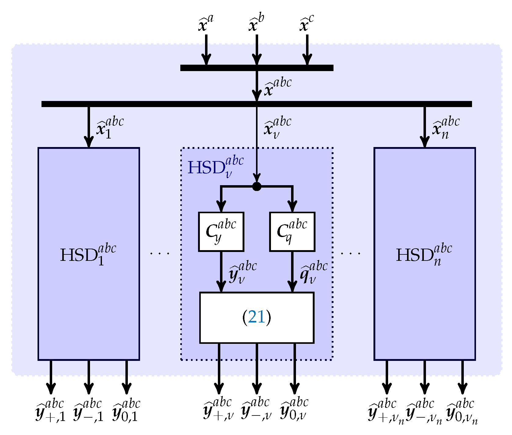
• positive-, negative-, and zero-sequence detection of each harmonic component and of the original low-pass filtered input signals (see Section 2.7); and
• Illustration of the theoretical results by extensive simulations (see Section 3).

1.1. Problem Statement

Here, we consider unbalanced (for unbalanced three-phase signals, the following holds $y^a\left(t\right)+y^b\left(t\right)+y^c\left(t\right)\ne 0$ at least for some time instant $t\ge 0$), three-phase systems or signals (of e.g., voltages or currents) with significant and arbitrary harmonic distortion (In this paper, all quantities of the phases a,b,c will be expressed as signal vectors of the form ${\mathit{y}}^{abc}\left(t\right)={\left(y^a\left(t\right),y^b\left(t\right),y^c\left(t\right)\right)}^{\top }\in {\mathbb{R}}^3$ for all $t\ge 0$, where $y\in \{v,i,\psi ,\cdots \}$ could represent e.g., voltage, current, or flux linkage). The considered systems consist of three phases, a, b, and c, and are described in compact vector notation by the following input (original) signal vector.

$$\forall t\ge 0:y^{abc}\left(t\right):=\left(\begin{array}{c}{y}^a\left(t\right)\\ y^b\left(t\right)\\ y^c\left(t\right)\end{array}\right):=\underset{=:y_{\mathrm{dc}}^{abc}\left(t\right)}{\underbrace{\left(\begin{array}{c}{a}_0^a\left(t\right)\\ a_0^b\left(t\right)\\ a_0^c\left(t\right)\end{array}\right)}}+\sum _{\nu \in {\mathbb{H}}_{\infty }}\underset{=:y_{\nu }^{abc}\left(t\right)}{\underbrace{\left(\begin{array}{c}{a}_{\nu }^a\left(t\right)cos\left({\varphi }_{\nu }^a\left(t\right)\right)\\ a_{\nu }^b\left(t\right)cos\left({\varphi }_{\nu }^b\left(t\right)\right)\\ a_{\nu }^c\left(t\right)cos\left({\varphi }_{\nu }^c\left(t\right)\right)\end{array}\right)}}\in {\mathbb{R}}^3;$$

(2)

where ${\mathbb{H}}_{\infty }:=\{1,{\nu }_2,\cdots ,{\nu }_{\infty }\}\subset {\mathbb{Q}}_{>0}$ with DC-offsets $a_0^p$, fundamental amplitude $a_1^p$, harmonic amplitudes $a_{{\nu }_2}^p,\cdots ,a_{{\nu }_{\infty }}^p\ge 0$, and angles ${\varphi }_{\nu }^p$ (in $\mathrm{rad}$), respectively; where $p\in \{a,b,c\}$ represents the superscript for the three phases a, b, and c and $\nu \in {\mathbb{H}}_{\infty }$ indicates the $\nu$-th harmonic component (per definition ${\nu }_1:=1$). Observe that $\nu$ does not necessarily need to be a natural number; non-zero rational numbers larger or smaller than one (e.g., $\nu ={\nu }_2=2/3$) are admissible as well to consider, e.g., inter-harmonics. Moreover, to consider the most general case, note that the phase angles

$$\forall p\in \{a,b,c\}\forall \nu \in {\mathbb{H}}_{\infty }\forall t\ge 0:{\varphi }_{\nu }^p\left(t\right)={\int }_0^t\underset{=:{\omega }_{\nu }^p\left(\tau \right)}{\underbrace{\nu {\omega }_1^p\left(\tau \right)}}\mathrm{d}\tau +{\varphi }_{0,\nu }^p$$

of the $\nu$-th harmonic component depend on the possibly time-varying angular fundamental frequency ${\omega }_1^p\left(·\right)>0\mathrm{rad}/\mathrm{s}$, and the initial angle ${\varphi }_{0,\nu }^p\in \mathbb{R}$. Both quantities are allowed to differ between the three phases $p\in \{a,b,c\}$ and the harmonic components. The main goal of this paper is twofold:

(i)

to detect online estimates of DC-offset ${\widehat{a}}_0^p$, amplitudes ${\widehat{a}}_{\nu }^p$, and angles ${\widehat{\varphi }}_{\nu }^p$ of the three phases $p\in \{a,b,c\}$ for a limited bandwidth of the total harmonic distortion—that is, $\nu \in {\mathbb{H}}_n:=\{1,{\nu }_2,\cdots ,{\nu }_n\}\subset {\mathbb{H}}_{\infty }$ (where, clearly, the highest harmonic ${\nu }_n$ is smaller than ${\nu }_{\infty }$—that is, ${\nu }_n<{\nu }_{\infty }$), such that, after a short transient phase, the estimated quantities (indicated by “ $\widehat{}$ ”) are equal to the band-limited (low-pass and high-pass filtered; see Section 2.1 and Section 2.2) original signal. More precisely, the following should hold:

$${\widehat{\mathit{y}}}^{abc}\left(t\right):=\underset{=:{\widehat{\mathit{y}}}_{\mathrm{dc}}^{abc}\left(t\right)}{\underbrace{\left(\begin{array}{c}{\widehat{a}}_0^a\left(t\right)\\ {\widehat{a}}_0^b\left(t\right)\\ {\widehat{a}}_0^c\left(t\right)\end{array}\right)}}+\sum _{\nu \in {\mathbb{H}}_n}\underset{=:{\widehat{\mathit{y}}}_{\nu }^{abc}\left(t\right)}{\underbrace{\left(\begin{array}{c}{\widehat{a}}_{\nu }^a\left(t\right)cos\left({\widehat{\varphi }}_{\nu }^a\left(t\right)\right)\\ {\widehat{a}}_{\nu }^b\left(t\right)cos\left({\widehat{\varphi }}_{\nu }^b\left(t\right)\right)\\ {\widehat{a}}_{\nu }^c\left(t\right)cos\left({\widehat{\varphi }}_{\nu }^c\left(t\right)\right)\end{array}\right)}}={\mathit{y}}_{\mathrm{dc}}^{abc}\left(t\right)+\sum _{\nu \in {\mathbb{H}}_n}{\mathit{y}}_{\nu }^{abc}\left(t\right);$$

(3)

(ii)

and if the fundamental frequencies of the three phases are identical (i.e., ${\omega }_1^a\left(t\right)={\omega }_1^b\left(t\right)={\omega }_1^c\left(t\right)$ for all $t\ge 0$), to extract, for each harmonic $\nu \in {\mathbb{H}}_n$, positive sequence components${\widehat{\mathit{y}}}_{+,\nu }^{abc}:={\left({\widehat{y}}_{+,\nu }^a,{\widehat{y}}_{+,\nu }^b,{\widehat{y}}_{+,\nu }^c\right)}^{\top }$, negative sequence components${\widehat{\mathit{y}}}_{-,\nu }^{abc}:={\left({\widehat{y}}_{-,\nu }^a,{\widehat{y}}_{-,\nu }^b,{\widehat{y}}_{-,\nu }^c\right)}^{\top }$ (Positive and negative sequences are balanced signals, that is, ${\widehat{y}}_x^a\left(t\right)+{\widehat{y}}_x^b\left(t\right)+{\widehat{y}}_x^c\left(t\right)=0$ for all $t\ge 0$ and $x\in \{+,-\}$ ([9], Appendix A)) and zero sequence components${\widehat{\mathit{y}}}_{0,\nu }^{abc}:={\left({\widehat{y}}_{0,\nu }^a,{\widehat{y}}_{0,\nu }^b,{\widehat{y}}_{0,\nu }^c\right)}^{\top }$ of the low-pass filtered and offset free harmonic signal vector $y_{\nu }^{abc}\left(·\right)$ as in (3) such that the following holds $y_{\nu }^{abc}\left(t\right)\stackrel{!}{=}{\widehat{\mathit{y}}}_{+,\nu }^{abc}\left(t\right)+{\widehat{\mathit{y}}}_{-,\nu }^{abc}\left(t\right)+{\widehat{\mathit{y}}}_{0,\nu }^{abc}\left(t\right)$ for all $\nu \in {\mathbb{H}}_n$ and $t\ge 0$ (at least in the steady-state).

Remark 1.

Note that in (2), time-varying phase amplitudes (of each harmonic component)andtime-varying phase angles are considered. The typical assumption (see, e.g., ([9], Appendix A)) of aconstantfundamental angular frequency ${\omega }_1^p>0$ with $p\in \{a,b,c\}$ such that ${\varphi }_{\nu }^p\left(t\right)=\nu {\omega }_1^{p}t$ is not imposed, since it is not generally true.

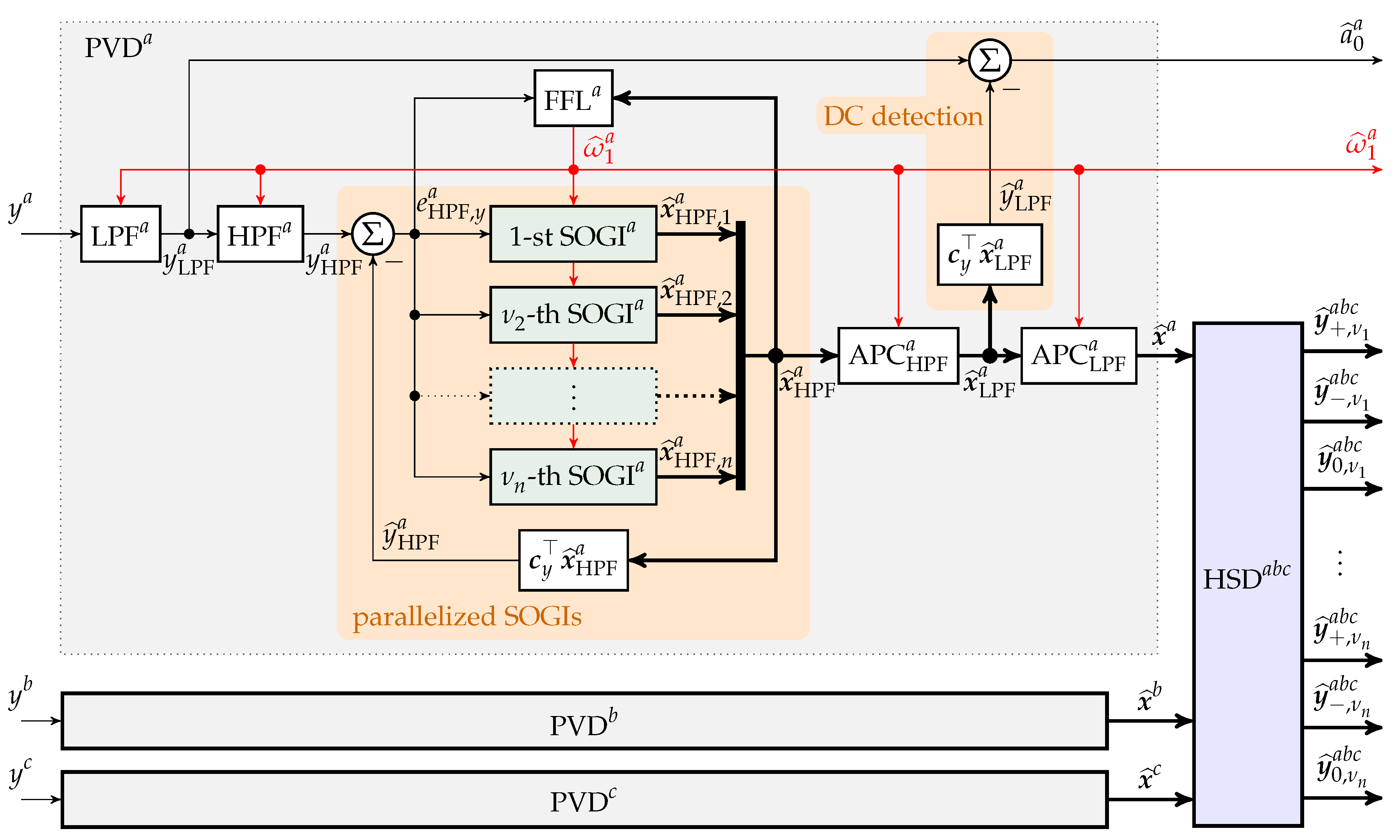
1.2. Principle Idea of Proposed Overall Solution

The principle idea of the proposed overall solution is illustrated in Figure 1. The depicted block diagram is fed by the input signals $y^a$, $y^b$, and $y^c$ of the respective phases $a,b,c$, and shows the individual phase variables detection (PVD${}^p$) blocks for the three phases $p\in \{a,b,c\}$ and the harmonic sequence detection (HSD${}^{abc}$). The outputs of the block diagram are the respective estimated signal components (see Section 1.1). In Figure 1, all components (sub-blocks) of PVD${}^a$ are explicitly shown. PVD${}^b$ and PVD${}^c$ have identical components. One can summarize: For $p\in \{a,b,c\}$ and $\nu \in {\mathbb{H}}_n$, each PVD${}^p$ consists of the following sub-blocks:

Figure 1. Overall block diagram of Phase Variables Detection (PVD) for the three phases $a,b,c$ and Harmonic Sequence Detection (HSD).

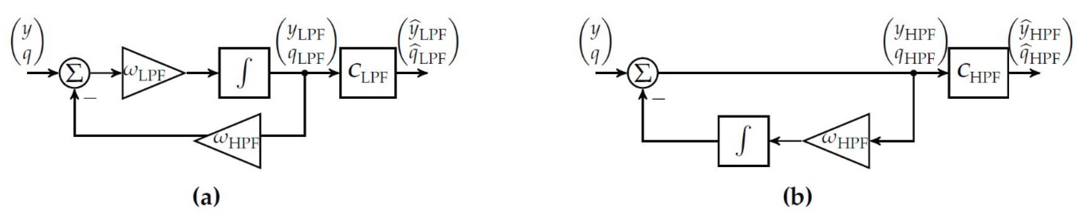
• A Low-Pass Filter (LPF${}^p$) to filter out noise and limit the bandwidth of the input signal $y^p$;
• A High-Pass Filter (HPF${}^p$) to filter out any DC-offset in the low-pass filtered signal $y_{\mathrm{LPF}}^p$;
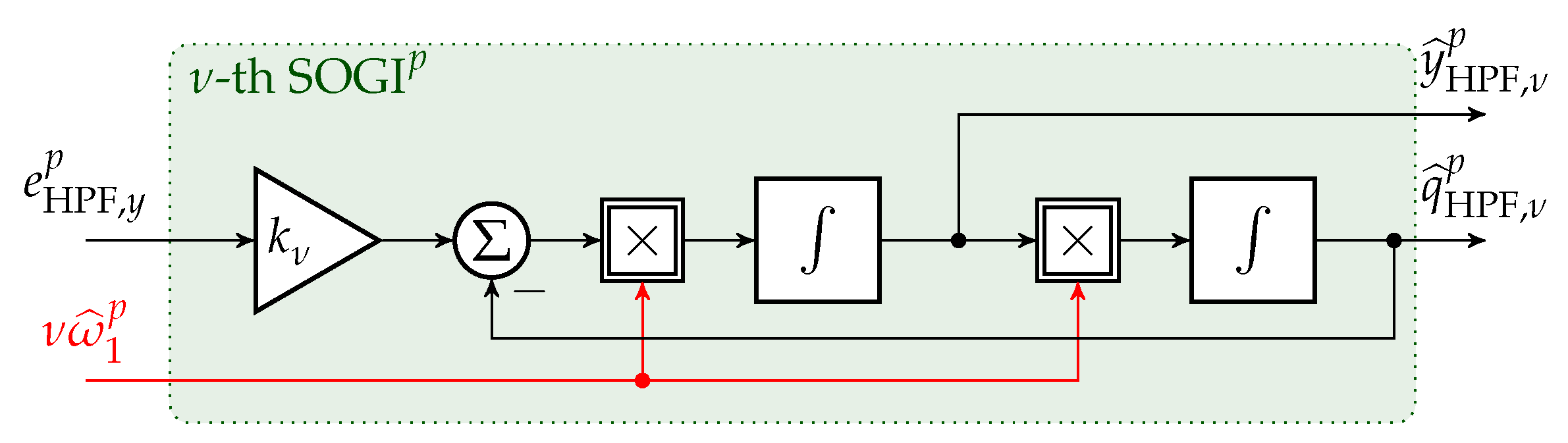
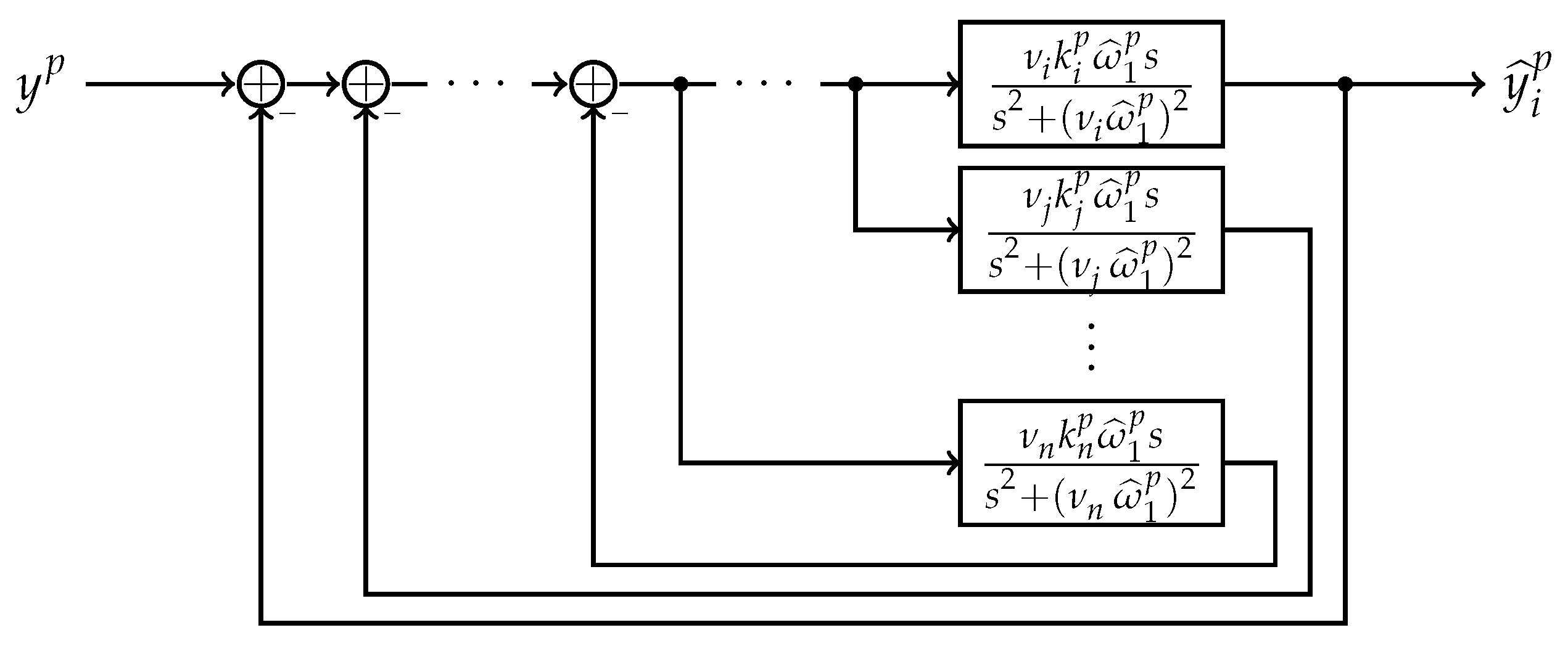
• A parallelization of Second-Order Generalized Integrators (SOGIs) to detect the amplitude and phase of each of the harmonic components of the high-pass filtered signal $y_{\mathrm{HPF}}^p$: the $\nu$-th SOGI${}^p$ will output the estimated signal vector ${\widehat{\mathit{x}}}_{\mathrm{HPF},\nu }^p:={({\widehat{y}}_{\mathrm{HPF},\nu }^p,{\widehat{q}}_{\mathrm{HPF},\nu }^p)}^{\top }$ compromising estimate of the direct and quadrature signal of the $\nu$-th harmonic, resp. All n-estimated signal vectors ${\widehat{\mathit{x}}}_{\mathrm{HPF},\nu }^p$ are merged into the overall estimate vector

  $${\widehat{\mathit{x}}}_{\mathrm{HPF}}^p:={\left(\underset{=:{\left({\widehat{\mathit{x}}}_{\mathrm{HPF},1}^p\right)}^{\top }}{\underbrace{{({\widehat{y}}_{\mathrm{HPF},1}^p,{\widehat{q}}_{\mathrm{HPF},1}^p)}^{\top }}},\underset{=:{\left({\widehat{\mathit{x}}}_{\mathrm{HPF},{\nu }_2}^p\right)}^{\top }}{\underbrace{{({\widehat{y}}_{\mathrm{HPF},{\nu }_2}^p,{\widehat{q}}_{\mathrm{HPF},{\nu }_2}^p)}^{\top }}},\cdots ,\underset{=:{\left({\widehat{\mathit{x}}}_{\mathrm{HPF},{\nu }_n}^p\right)}^{\top }}{\underbrace{{({\widehat{y}}_{\mathrm{HPF},{\nu }_n}^p,{\widehat{q}}_{\mathrm{HPF},{\nu }_n}^p)}^{\top }}}\right)}^{\top }\in {\mathbb{R}}^{2n}.$$

  (4)
  The overall estimate output ${\widehat{y}}_{\mathrm{HPF}}^p={\sum }_{\nu \in {\mathbb{H}}_n}{\widehat{y}}_{\mathrm{HPF},\nu }^p={\mathit{c}}_y^{\top }{\widehat{\mathit{x}}}_{\mathrm{HPF}}^p$ of the SOGI input signal $y_{\mathrm{HPF}}^p$ is established by the sum (linear combination) of the estimates of the direct signals of all SOGIs;
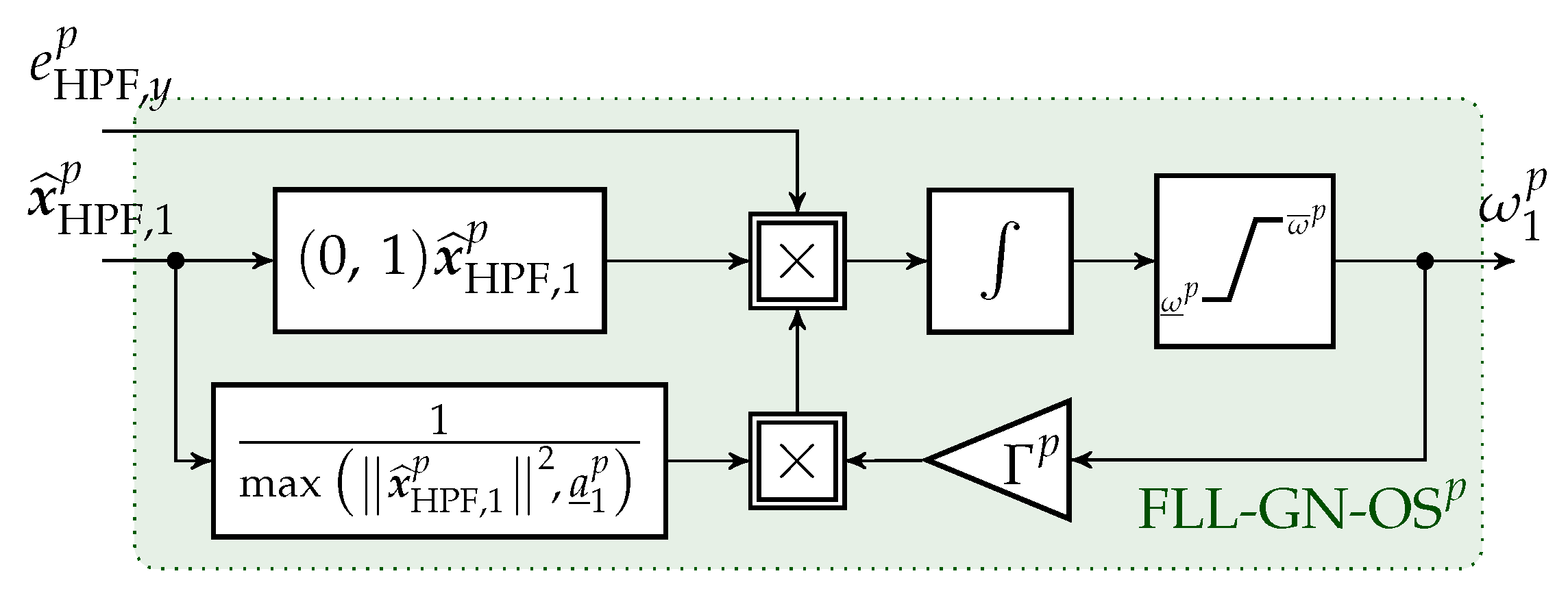
• a Frequency-Locked Loop (FLL${}^p$) to obtain the estimate ${\widehat{\omega }}_1^p$ of the fundamental angular frequency ${\omega }_1^p$ of the high-pass filtered signal $y_{\mathrm{HPF}}^p$;
• an Amplitude Phase Correction (APC${}_{\mathrm{x}}^p$ with $\mathrm{x}\in \{\mathrm{LPF},\mathrm{HPF}\}$) to mitigate for amplitude damping and phase shift introduced by LPF${}^p$ and HPF${}^p$, resp.: The merged estimated signal vector ${\widehat{\mathit{x}}}_{\mathrm{HPF}}^p$ of the parallelized SOGIs is fed into the APC${}_{\mathrm{HPF}}^p$. The  APC${}_{\mathrm{HPF}}^p$ output vector

  $${\widehat{\mathit{x}}}_{\mathrm{LPF}}^p={\left(\underset{=:{\left({\widehat{\mathit{x}}}_{\mathrm{LPF},1}^p\right)}^{\top }}{\underbrace{{({\widehat{y}}_{\mathrm{LPF},1}^p,{\widehat{q}}_{\mathrm{LPF},1}^p)}^{\top }}},\underset{=:{\left({\widehat{\mathit{x}}}_{\mathrm{LPF},{\nu }_2}^p\right)}^{\top }}{\underbrace{{({\widehat{y}}_{\mathrm{LPF},{\nu }_2}^p,{\widehat{q}}_{\mathrm{LPF},{\nu }_2}^p)}^{\top }}},\cdots ,\underset{=:{\left({\widehat{\mathit{x}}}_{\mathrm{LPF},{\nu }_n}^p\right)}^{\top }}{\underbrace{{({\widehat{y}}_{\mathrm{LPF},{\nu }_n}^p,{\widehat{q}}_{\mathrm{LPF},{\nu }_n}^p)}^{\top }}}\right)}^{\top }\in {\mathbb{R}}^{2n}$$

  (5)

  comprises all amplitude-correct and phase-correct direct and quadrature estimates of the low-pass filtered signal $y_{\mathrm{LPF}}^p$ (see Figure 1). The signal vector ${\widehat{\mathit{x}}}_{\mathrm{LPF}}^p$ is fed into the APC${}_{\mathrm{LPF}}^p$ to reconstruct amplitude-correct and phase-correct direct and quadrature estimates of the original signal $y^p$ (see Figure 1). The output vector of the APC${}_{\mathrm{LPF}}^p$ is given by

  $${\widehat{\mathit{x}}}^p={\left(\underset{=:{\left({\widehat{\mathit{x}}}_1^p\right)}^{\top }}{\underbrace{{({\widehat{y}}_1^p,{\widehat{q}}_1^p)}^{\top }}},\underset{=:{\left({\widehat{\mathit{x}}}_{{\nu }_2}^p\right)}^{\top }}{\underbrace{{({\widehat{y}}_{{\nu }_2}^p,{\widehat{q}}_{{\nu }_2}^p)}^{\top }}},\cdots ,\underset{=:{\left({\widehat{\mathit{x}}}_{{\nu }_n}^p\right)}^{\top }}{\underbrace{{({\widehat{y}}_{{\nu }_n}^p,{\widehat{q}}_{{\nu }_n}^p)}^{\top }}}\right)}^{\top }\in {\mathbb{R}}^{2n}.$$

  (6)
• A DC-offset detection to obtain an estimate ${\widehat{a}}_0^p$ of the DC-offset $a_0^p$ in the original signal $y^p$ (see Figure 1).

The output vectors ${\widehat{\mathit{x}}}^a$, ${\widehat{\mathit{x}}}^b$, and ${\widehat{\mathit{x}}}^c$ of the three PVDs (see Figure 1) are fed into the HSD${}^{abc}$ block, which finally extracts positive-, negative-, and zero-sequence vectors ${\widehat{\mathit{y}}}_{+,\nu }^{abc}$, ${\widehat{\mathit{y}}}_{-,\nu }^{abc}$, and ${\widehat{\mathit{y}}}_{0,\nu }^{abc}$ of each harmonic $\nu \in {\mathbb{H}}_n$. Each block and its function are explained in the following section. In the appendix, a thorough stability analysis of the closed-loop system (parallelized SOGIs with FLL) is presented.

Remark 2.

If the three phases can be considered to have a similar frequency content and the same frequency, then only one FFL is required. Moreover, the LPFs, HPFs, and the corresponding APCs can be designed identically.

2. Detailed Discussion of Proposed Overall Solution

This section introduces the different sub-blocks illustrated in Figure 1 and describes their contribution to the proposed overall solution to detect individual phase variables and positive-, negative-, and zero-sequence components of all harmonics $\nu \in {\mathbb{H}}_n$ of the input signal(s).

2.1. Low-Pass Filter (Bandwidth Limitation and Noise Filtering)

For each phase $p\in \{a,b,c\}$, a first-order, low-pass filter (LPF) is introduced to filter out noise and limit the bandwidth of the original signal $y^p$ up to the n-th harmonic component. The filter dynamics are given by

$$\left.\begin{array}{ccc}\hfill \frac{\mathrm{d}}{\mathrm{d}t}{\xi }_{\mathrm{LPF}}^p\left(t\right)& =& {\omega }_{\mathrm{LPF}}^p\left(t\right)\left(-{\xi }_{\mathrm{LPF}}^p\left(t\right)+y^p\left(t\right)\right),{\xi }_{\mathrm{LPF}}^p\left(0\right)=0\hfill \\ \hfill y_{\mathrm{LPF}}^p\left(t\right)& =& {\xi }_{\mathrm{LPF}}^p\left(t\right),\hfill \end{array}\right\}$$

(7)

where $y_{\mathrm{LPF}}^p$ and ${\omega }_{\mathrm{LPF}}^p$ (in $\mathrm{rad}/\mathrm{s}$) are the filter output and (possibly time-varying) cut-off angular frequency of the LPF, respectively. The LPF is stable for any uniformly positive cut-off frequency.

The cut-off frequency ${\omega }_{\mathrm{LPF}}^p\left(·\right)$ should be chosen such that, for a given sampling frequency $f_{\mathrm{s}}$ (in $\mathrm{Hz}$), Shannon’s Theorem is satisfied and the bandwidth is limited to a value specified by a desired magnitude damping factor $\epsilon \in (0,1)$ for the ${\nu }_{n+1}$-th harmonic (a low-pass filter $F\left(s\right)=\frac{{\omega }_{\mathrm{lpf}}^p}{s+{\omega }_{\mathrm{lpf}}^p}$ (that has a constant cut-off frequency) has the magnitude damping $\left|F(j\omega )\right|=\frac{{\omega }_{\mathrm{lpf}}^p}{\sqrt{{\omega }^2+{\left({\omega }_{\mathrm{lpf}}^p\right)}^2}}$). That is,     

$$\frac{{\omega }_{\mathrm{lpf}}^p}{\sqrt{{\left({\nu }_{n+1}{\widehat{\omega }}_1^p\right)}^2+{\left({\omega }_{\mathrm{lpf}}^p\right)}^2}}\le \epsilon ⟹0<{\omega }_{\mathrm{lpf}}^p\le \frac{\epsilon }{\sqrt{1-{\epsilon }^2}}{\nu }_{n+1}{\widehat{\omega }}_1^p\ll 2\pi f_{\mathrm{s}}.$$

(8)

Since the estimate ${\widehat{\omega }}_1^p$ of the fundamental angular frequency (see Section 2.4) will change over time, the choice of ${\omega }_{\mathrm{LPF}}^p$ will also be time-varying to obtain a respective bandwidth limitation depending on the fundamental angular frequency estimate ${\widehat{\omega }}_1^p$. For some constants $k_{\mathrm{LPF}}\ge 1$, a reasonable choice is ${\omega }_{\mathrm{LPF}}^p\left(t\right)=\frac{\epsilon }{k_{\mathrm{LPF}}\sqrt{1-{\epsilon }^2}}{\nu }_{n+1}{\widehat{\omega }}_1^p\left(t\right)$. Note that a very small desired damping (i.e., $\epsilon \ll 1$) implies a long settling of the LPF and additional noise filtering, which is not necessary since the following SOGIs filter out noise as well [21].

2.2. High-Pass Filter (Suppression of DC-Offset)

A first-order high-pass filter (HPF) is introduced for each phase $p\in \{a,b,c\}$ to suppress any DC-offset in the low-pass filtered input signal $y_{\mathrm{LPF}}^p$. The HPF dynamics are given by

$$\left.\begin{array}{ccc}\hfill \frac{\mathrm{d}}{\mathrm{d}t}{\xi }_{\mathrm{HPF}}^p\left(t\right)& =& {\omega }_{\mathrm{HPF}}^p\left(t\right)\left(-{\xi }_{\mathrm{HPF}}^p\left(t\right)+y_{\mathrm{LPF}}^p\left(t\right)\right),{\xi }_{\mathrm{HPF}}^p\left(0\right)=0\hfill \\ \hfill y_{\mathrm{HPF}}^p\left(t\right)& =& -{\xi }_{\mathrm{HPF}}^p\left(t\right)+y_{\mathrm{LPF}}^p\left(t\right),\hfill \end{array}\right\}$$

(9)

where $y_{\mathrm{HPF}}^p$ and ${\omega }_{\mathrm{HPF}}^p$ (in $\mathrm{rad}/\mathrm{s}$) are the DC-free output (after a transient phase) (see Figure 1) and the (possibly time-varying) cut-off angular frequency of the HPF, respectively. The HPF is stable for any uniformly positive cut-off frequency. The cut-off frequency must be chosen (much) smaller than the sampling frequency $f_{\mathrm{s}}$ (see above)—that is, ${\omega }_{\mathrm{HPF}}^p\left(t\right)\ll 2\pi f_{\mathrm{s}}$ for all $t\ge 0$.

2.3. Second-Order Generalized Integrator (SOGI)

This section introduces the key tool for the detection of phase variables: A second-order generalized integrator (SOGI), which is a special kind of internal model to reduplicate sinusoidal signals [41]. Their parallelization in combination with the frequency-locked loop (see Section 2.4) will allow detection of the variables for each harmonic component.

2.3.1. SOGI for the $\nu$-th Harmonic Component of Phase $p\in \{a,b,c\}$

For now, let $\nu \in {\mathbb{H}}_n$, and consider only the $\nu$-th harmonic component $y_{\mathrm{HPF},\nu }^p\left(t\right):=a_{\mathrm{HPF},\nu }^p\left(t\right)cos\left({\varphi }_{\mathrm{HPF},\nu }^p\left(t\right)\right)$. If the estimate ${\widehat{\omega }}_{\nu }^p:=\nu {\widehat{\omega }}_1^p$ of the $\nu$-th harmonic frequency is known (e.g., the fundamental is known, then ${\widehat{\omega }}_1^p={\omega }_1^p$), the implementation of a SOGI for the signal $y_{\mathrm{HPF},\nu }^p\left(·\right)$ allows to obtain online estimates ${\widehat{y}}_{\mathrm{HPF},\nu }^p\left(·\right)$ and ${\widehat{q}}_{\mathrm{HPF},\nu }^p\left(·\right)$ of the input (direct) signal and its quadrature signal, respectively. A SOGI for the $\nu$-th harmonic component is depicted in Figure 2.

Figure 2. Block diagram of a Second-Order Generalized Integrator (SOGI) for the detection of the $\nu$-th harmonic component.

Its dynamics are given by the following time-varying second-order differential equation ([9], Appendix A):

$$\frac{\mathrm{d}}{\mathrm{d}t}\underset{=:{\widehat{\mathit{x}}}_{\mathrm{HPF},\nu }^p\left(t\right)\in {\mathbb{R}}^2}{\underbrace{\left(\begin{array}{c}{\widehat{y}}_{\mathrm{HPF},\nu }^p\left(t\right)\\ {\widehat{q}}_{\mathrm{HPF},\nu }^p\left(t\right)\end{array}\right)}}=\underset{=:{\widehat{\omega }}_{\nu }^p\left(t\right)}{\underbrace{\nu {\widehat{\omega }}_1^p\left(t\right)}}\underset{=:{\mathit{A}}_{\nu }^p\in {\mathbb{R}}^{2\times 2}}{\underbrace{\left[\begin{array}{cc}-k_{\nu }^p& -1\\ 1& 0\end{array}\right]}}{\widehat{\mathit{x}}}_{\mathrm{HPF},\nu }^p\left(t\right)+{\widehat{\omega }}_{\nu }^p\left(t\right)\underset{=:{\mathit{b}}_{\nu }^p}{\underbrace{\left(\begin{array}{c}{k}_{\nu }^p\\ 0\end{array}\right)}}{y}_{\mathrm{HPF},\nu }^p\left(t\right),k_{\nu }^p>0;$$

(10)

with arbitrary initial value ${\widehat{\mathit{x}}}_{\nu }^p\left(0\right)={\widehat{\mathit{x}}}_{0,\nu }^p\in {\mathbb{R}}^2$ (most likely, ${\widehat{\mathit{x}}}_{0,\nu }^p={\mathbf{0}}_2$ is a reasonable choice) and possibly time-varying angular frequency ${\widehat{\omega }}_{\nu }\left(·\right)$. The gain $k_{\nu }^p$ allows for tuning of the dynamical response of the SOGI. For a constant frequency ${\widehat{\omega }}_{\nu }^p$ only, the characteristic equation and the SOGI poles are given as follows:

$${\chi }_{\nu }\left(s\right):=det\left[s{\mathit{I}}_2-{\widehat{\omega }}_{\nu }^p{\mathit{A}}_{\nu }^p\right]=s^2+k_{\nu }^p{\widehat{\omega }}_{\nu }^{p}s+{\left({\widehat{\omega }}_{\nu }^p\right)}^2\stackrel{!}{=}0⟹p_{\nu ,1/2}^p=-\frac{k_{\nu }^p{\widehat{\omega }}_{\nu }^p}{2}\left(1\pm \sqrt{1-\frac{4}{{\left(k_{\nu }^p\right)}^2}}\right).$$

(11)

So, for a constant frequency only (note that for time-varying or nonlinear systems, the analysis of poles is not sufficient to check stability ([42], Example 3.3.7)) and only one SOGI, stability is guaranteed for $k_{\nu }^p>0$. It will be shown later that this stability statement also holds true for the parallelized SOGIs (see Appendix A.1). For $0<k_{\nu }^p\le 2$, an over-damped system response is obtained (i.e., imaginary parts of the poles are zero). The estimated amplitude ${\widehat{a}}_{\mathrm{HPF},\nu }^p\left(t\right):=∥{\widehat{\mathit{x}}}_{\mathrm{HPF},\nu }^p\left(t\right)∥=\sqrt{{\widehat{y}}_{\mathrm{HPF},\nu }^p{\left(t\right)}^2+{\widehat{q}}_{\mathrm{HPF},\nu }^p{\left(t\right)}^2}$ is given by the norm of the estimated signal and its quadrature signal and the estimated phase angle by ${\widehat{\varphi }}_{\mathrm{HPF},\nu }^p\left(t\right)=arctan2\left({\widehat{y}}_{\mathrm{HPF},\nu }^p\left(t\right),{\widehat{q}}_{\mathrm{HPF},\nu }^p\left(t\right)\right)$. In conclusion, the phase variables ${\widehat{a}}_{\mathrm{HPF},\nu }^p$ and ${\widehat{\varphi }}_{\mathrm{HPF},\nu }^p$ can be detected online.

2.3.2. Parallelization of SOGIs

Since only one harmonic component can be detected with one SOGI, it is straightforward to implement SOGIs for different harmonic components in parallel. Moreover, note that for the low- & high-pass filtered input signal $y_{\mathrm{HPF}}^p\left(·\right)$ (see Figure 1) with $p\in \{a,b,c\}$, the harmonic component $y_{\mathrm{HPF},\nu }^p\left(·\right)$ as in (10) is not available for implementation. However, it may be approximated by

$$y_{\mathrm{HPF},\nu }^p\left(t\right)\approx y_{\mathrm{HPF}}^p\left(t\right)-\sum _{\begin{array}{c}k=1\\ k\ne \nu \end{array}}^n{\widehat{y}}_{\mathrm{HPF},k}^p\left(t\right)\stackrel{\left(10\right)}{\Rightarrow }{\widehat{\omega }}_{\nu }^p\left(t\right){\mathit{b}}_{\nu }^p{y}_{\mathrm{HPF},\nu }^p\left(t\right)\approx {\widehat{\omega }}_{\nu }^p\left(t\right){\mathit{b}}_{\nu }^p{y}_{\mathrm{HPF}}^p\left(t\right)-{\widehat{\omega }}_{\nu }^p\left(t\right)\underset{=:{\mathit{K}}_{\nu }^p}{\underbrace{{\mathit{b}}_{\nu }^p\left(1,0\right)}}\sum _{\begin{array}{c}k\in {\mathbb{H}}_n\\ k\ne \nu \end{array}}{\widehat{\mathit{x}}}_{\mathrm{HPF},k}^p\left(t\right),$$

(12)

where ${\widehat{y}}_{\mathrm{HPF},k}^p$ is the estimated signal and ${\widehat{\mathit{x}}}_{\mathrm{HPF},k}^p\left(t\right)$ is the state vector of the k-th SOGI as in (10). Clearly, this leads to the parallelization of n SOGIs, as illustrated in Figure 1 (see highlighted box, “parallelized SOGIs”). The dynamics of the parallelized SOGIs are given by a $2n$-th order time-varying differential equation as follows:

$$\begin{array}{ccc}\hfill \frac{\mathrm{d}}{\mathrm{d}t}\underset{=:{\widehat{\mathit{x}}}_{\mathrm{HPF}}^p\left(t\right)}{\underbrace{\left(\begin{array}{c}{\widehat{\mathit{x}}}_{\mathrm{HPF},1}^p\left(t\right)\\ ⋮\\ {\widehat{\mathit{x}}}_{\mathrm{HPF},n}^p\left(t\right)\end{array}\right)}}& =& \left[\begin{array}{ccc}{\widehat{\omega }}_1^p\left(t\right){\mathit{A}}_1^p& \cdots & -{\widehat{\omega }}_1^p\left(t\right){\mathit{K}}_1^p\\ ⋮& \ddots & ⋮\\ -{\widehat{\omega }}_n^p\left(t\right){\mathit{K}}_n^p& \cdots & {\widehat{\omega }}_n^p\left(t\right){\mathit{A}}_n^p\end{array}\right]{\widehat{\mathit{x}}}_{\mathrm{HPF}}^p\left(t\right)+\left(\begin{array}{c}{\widehat{\omega }}_1^p\left(t\right){\mathit{b}}_1^p\\ ⋮\\ {\widehat{\omega }}_n^p\left(t\right){\mathit{b}}_n^p\end{array}\right)y_{\mathrm{HPF}}^p\left(t\right)\hfill \\ \hfill & =& {\widehat{\omega }}_1^p\left(t\right)\left(\left[\begin{array}{ccccc}-k_1^p& -1& \cdots & -k_1^p& 0\\ 1& 0& \cdots & 0& 0\\ ⋮& ⋮& \ddots & ⋮& ⋮\\ -{\nu }_n{k}_n^p& 0& \cdots & -{\nu }_n{k}_n^p& -{\nu }_n\\ 0& 0& \cdots & {\nu }_n& 0\end{array}\right]{\widehat{\mathit{x}}}_{\mathrm{HPF}}^p\left(t\right)+\left(\begin{array}{c}{k}_1^p\\ 0\\ ⋮\\ {\nu }_n{k}_n^p\\ 0\end{array}\right)y_{\mathrm{HPF}}^p\left(t\right)\right)\hfill \\ \hfill & =& {\widehat{\omega }}_1^p\left(t\right)\underset{=:{\mathit{A}}^p\in {\mathbb{R}}^{2n\times 2n}}{\underbrace{\left[\begin{array}{ccc}\overline{\mathit{J}}-{\mathit{K}}_1^p& \cdots & -{\mathit{K}}_1^p\\ ⋮& \ddots & ⋮\\ -{\nu }_n{\mathit{K}}_n^p& \cdots & {\nu }_n\left(\overline{\mathit{J}}-{\mathit{K}}_n^p\right)\end{array}\right]}}{\widehat{\mathit{x}}}_{\mathrm{HPF}}^p\left(t\right)+\underset{=:{\mathit{b}}^p\in {\mathbb{R}}^{2n}}{\underbrace{\left(\begin{array}{c}{k}_1^p\\ 0\\ ⋮\\ {\nu }_n{k}_n^p\\ 0\end{array}\right)}}{y}_{\mathrm{HPF}}^p\left(t\right).\hfill \end{array}$$

(13)

Note that matrix ${\mathit{A}}^p$ and vector ${\mathit{b}}^p$ are constant; nevertheless, due to a possibly time-varying estimate ${\widehat{\omega }}_1^p\left(·\right)$ of the fundamental angular frequency, the overall dynamics of the parallelized SOGIs are time-varying. The output of the parallelized SOGI system is the direct component of the estimated signal—that is, 

$${\widehat{y}}_{\mathrm{HPF}}^p\left(t\right)=\underset{=:{\mathit{c}}_y^{\top }\in {\mathbb{R}}^{2n}}{\underbrace{\left(\begin{array}{c}1,0,1,0,\cdots ,1,0\end{array}\right)}}{\widehat{\mathit{x}}}_{\mathrm{HPF}}^p\left(t\right).$$

(14)

The linear combination of the estimated quadrature signals is given by

$${\widehat{q}}_{\mathrm{HPF}}^p\left(t\right)=\underset{=:{\mathit{c}}_q^{\top }\in {\mathbb{R}}^{2n}}{\underbrace{\left(\begin{array}{c}0,1,0,1,\cdots ,0,1\end{array}\right)}}{\widehat{\mathit{x}}}_{\mathrm{HPF}}^p\left(t\right).$$

(15)

In the Appendix A, it is shown that system (13) of the parallelized SOGIs has the following properties: (i) It is bounded-input bounded-state/output (BIBS/O) stable—that is, there exists $c_v>0$ such that $∥{\widehat{\mathit{x}}}_{\mathrm{HPF}}^p\left(t\right)∥\le c_v{\parallel y_{\mathrm{HPF}}^p\parallel }_{\infty }$ for all $t\ge 0$ (see Theorem A2), and (ii) it asymptotically tracks the input signal $y_{\mathrm{HPF}}^p$—that is, ${lim}_{t\to \infty }\left(y_{\mathrm{HPF}}^p\left(t\right)-{\widehat{y}}_{\mathrm{HPF}}^p\left(t\right)\right)=0$, if (a) the matrix ${\mathit{A}}^p$ is Hurwitz and (b) the estimated and actual fundamental frequency is equal on some interval ${\mathbb{I}}_{\mathrm{ss}}\subseteq {\mathbb{R}}_{\ge 0}$ (i.e., ${\widehat{\omega }}_1^p\left(t\right)={\omega }_1^p\left(t\right)$ for all $t\in {\mathbb{I}}_{\mathrm{ss}}$; see Theorem A3).

2.3.3. Tuning of the SOGIs

Tuning is important in terms of settling time. Regarding the poles (eigenvalues) of ${\mathit{A}}^p$, the biggest real part of the poles defines the settling time; the corresponding pole is called a dominant pole. A common way of tuning parallelized SOGIs is $\mathit{b}={\mathit{c}}_y$ [13]; a more general and intuitive way is $\mathit{b}=g{\mathit{c}}_y$ with $g>0$. An analysis of the real parts in these cases shows that the dominant pole is close to the imaginary axis, which implies a slow settling. Therefore, a new tuning method is proposed, which finds the parameters $k_1,\dots ,k_n$ in (13) for the minimal dominant pole of ${\mathit{A}}^p$, and is based on the gradient search ([43], p. 366). The respective Matlab code is shown in Appendix A.5.

As a validation, Table 2 shows the dominant poles for several tunings. As an outcome, the proposed tuning method decreases the dominant pole significantly, which leads to a faster settling response.

Table 2. Dominant poles for different tunings ($n=10$).

Tuning	Real Part of Dominant Pole
$\mathit{b}=\frac{1}{2}{\mathit{c}}_y$	$-0.135031721112582$
$\mathit{b}={\mathit{c}}_y$	$-0.0975625042839749$
$\mathit{b}=\sqrt{2}{\mathit{c}}_y$	$-0.0729803842851082$
$\mathit{b}$ as in Appendix A.5	$-0.303890132318627$

2.4. Frequency-Locked Loop (FLL) with Gain Normalization and Output Saturation

As illustrated above, a correct estimate of the fundamental angular frequency is essential for a proper functionality of the signal detection. In this section, the intuition of the working principle of a FLL is briefly re-visited, and afterward extended by gain normalization and output saturation.

2.4.1. Intuition behind a FLL

As shown in Figure 1, any of the SOGIs requires a “reference angular frequency”—that is, the fundamental frequency estimate ${\widehat{\omega }}_1^p$, to work properly. To illustrate the intuition behind the working principle of a FLL, assume that the input signal has a constant angular frequency ${\omega }_1^p$ within some time interval $\left[t_0,t_1\right]$, and only the fundamental components are considered. Then, in a steady-state only, the fundamental component error $e_{\mathrm{HPF},y,1}^p\left(t\right)$, whose amplitude sign is dependent on the frequency errors sign, is in-phase, with the fundamental component of the fundamental quadrature output ${\widehat{q}}_{\mathrm{HPF},1,1}^p\left(t\right)$, whose amplitude sign has no dependency on the frequency error. Thus, a straightforward adaption law can be formulated as:

$$\begin{array}{c}\hfill \frac{\mathrm{d}}{\mathrm{d}t}{\widehat{\omega }}_1^p\left(t\right)=-{\gamma }^p{\widehat{q}}_{\mathrm{HPF},1}^p\left(t\right)e_{\mathrm{HPF},y}^p\left(t\right)\approx -{\gamma }^p{\widehat{q}}_{\mathrm{HPF},1,1}^p\left(t\right)e_{\mathrm{HPF},y,1}^p\left(t\right),{\widehat{\omega }}_1^p\left(0\right)>0\end{array}$$

(16)

with some gain ${\gamma }^p>0$. The FLL can be extended by the commonly used Gain Normalization (GN) [9] to desensitize the FLL to fundamental amplitude and frequency uncertainties; therefore, ${\gamma }^p$ is specified as

$$\frac{\mathrm{d}}{\mathrm{d}t}{\widehat{\omega }}_1^p\left(t\right)=-\underset{=:\gamma \left(t\right)}{\underbrace{\frac{{\widehat{\omega }}_1^p\left(t\right){\mathsf{\Gamma }}^p}{max\left({∥{\widehat{\mathit{x}}}_{\mathrm{HPF},1}^p\left(t\right)∥}^2,{\underline{a}}_1^p\right)}}}{\widehat{q}}_{\mathrm{HPF},1}^p\left(t\right)e_{\mathrm{HPF},y}^p\left(t\right),{\widehat{\omega }}_1^p\left(0\right)>0$$

(17)

with some constant ${\mathsf{\Gamma }}^p>0$ ([9], Section 4.6); it should be chosen such that the FLL dynamic is slow compared to the SOGI dynamics, since it is based on steady-state observations. In (17), the denominator might get zero, so it has to be essentially bounded away from zero by some ${\underline{a}}_1^p>0$. Clearly, this adaption makes the overall dynamics of SOGI and FLL nonlinear, and stability analysis becomes quite tricky. To the best knowledge of the authors, only linearized and/or steady-state stability analyses exist. In this paper, we present bounded-input, bounded-state/output (BIBS/O) stability—that is, there exists $c_v>0$ such that $∥{\widehat{\mathit{x}}}_{\mathrm{HPF}}^p\left(t\right)∥\le c_v{\parallel y_{\mathrm{HPF}}^p\parallel }_{\infty }$ for all $t\ge 0$ (see Theorem A2), and (ii) asymptotic tracking of the input signal $y_{\mathrm{HPF}}^p$—that is, ${lim}_{t\to \infty }\left(y_{\mathrm{HPF}}^p\left(t\right)-{\widehat{y}}_{\mathrm{HPF}}^p\left(t\right)\right)=0$, if (a) the matrix ${\mathit{A}}^p$ is Hurwitz and (b) the estimated and actual fundamental frequency are equal on some interval ${\mathbb{I}}_{\mathrm{ss}}\subseteq {\mathbb{R}}_{\ge 0}$ (i.e., ${\widehat{\omega }}_1^p\left(t\right)={\omega }_1^p\left(t\right)$ for all $t\in {\mathbb{I}}_{\mathrm{ss}}$; see Theorem A3) of the parallelized SOGIs (13).

2.4.2. Output Saturation

The most severe case for the SOGI-FLL are negative frequencies, since this might lead to instability of the overall system; moreover, a frequency equal to zero will stop the FLL from working, due to the GN (see (17)). In conclusion, the estimated angular frequency must be kept positive for proper functionality, which can be achieved by an output saturation (OS), which limits the frequency to a lower boundary ${\underline{\omega }}^p>0$. Since the frequency usually lies within a certain range, additionally, an upper boundary ${\overline{\omega }}^p>0$ can be used. In [37], the authors already proposed an output saturation; however, they did not include a Gain Normalization as in [9], but extended the OS by an anti-windup strategy with a feedback gain, which, in the opinion of the authors, can destabilize the FLL (but not the SOGI!). The FLL, including a GN and OS (FLL-GN-OS), is shown in Figure 3.

Figure 3. Frequency Locked Loop with Gain Normalization and Output Saturation (FLL-GN-OS).

2.5. Amplitude and Phase Correction (APC) for Low-Pass Filter and High-Pass Filter

Since any filtering, due to a LPF or HPF, leads to a damping and phase shift of the filtered signal, amplitude and phase corrections are crucial for an amplitude-correct and phase-correct signal estimation. Basically, for each phase $p\in \{a,b,c\}$ and each harmonic $\nu \in {\mathbb{H}}_n$, the amplitude and phase of an estimated direct ${\widehat{y}}_{\mathrm{HPF},\nu }^p$ and quadrature ${\widehat{q}}_{\mathrm{HPF},\nu }^p$ signal can be corrected (at least in the steady-state) by rotating and scaling the respective APC input signal vectors ${\widehat{\mathit{x}}}_{\mathrm{HPF}}^p\left(·\right)$ and ${\widehat{\mathit{x}}}_{\mathrm{LPF}}^p\left(·\right)$ (see Figure 1). More precisely, the respective amplitude and phase corrections (i.e., APC${}_{\mathrm{HPF}}$ and APC${}_{\mathrm{LPF}}$) for HPF and LPF are achieved by the following linear transformations:

$$\forall p\in \{a,b,c\}:{\widehat{\mathit{x}}}_{\mathrm{LPF}}^p\left(t\right)=\underset{=:{\mathit{C}}_{\mathrm{HPF}}\left(t\right)\in {\mathbb{R}}^{2n\times 2n}}{\underbrace{\left[\begin{array}{cccc}{\mathit{C}}_{\mathrm{HPF},1}\left(t\right)& {\mathit{O}}_{2\times 2}& \cdots & {\mathit{O}}_{2\times 2}\\ {\mathit{O}}_{2\times 2}& {\mathit{C}}_{\mathrm{HPF},{\nu }_2}\left(t\right)& \ddots & ⋮\\ ⋮& \ddots & \ddots & {\mathit{O}}_{2\times 2}\\ {\mathit{O}}_{2\times 2}& \cdots & {\mathit{O}}_{2\times 2}& {\mathit{C}}_{\mathrm{HPF},{\nu }_n}\left(t\right)\end{array}\right]}}{\widehat{\mathit{x}}}_{\mathrm{HPF}}^p\left(t\right)$$

(18)

and

$$\forall p\in \{a,b,c\}:{\widehat{\mathit{x}}}^p\left(t\right)=\underset{=:{\mathit{C}}_{\mathrm{LPF}}\left(t\right)\in {\mathbb{R}}^{2n\times 2n}}{\underbrace{\left[\begin{array}{cccc}{\mathit{C}}_{\mathrm{LPF},1}\left(t\right)& {\mathit{O}}_{2\times 2}& \cdots & {\mathit{O}}_{2\times 2}\\ {\mathit{O}}_{2\times 2}& {\mathit{C}}_{\mathrm{LPF},{\nu }_2}\left(t\right)& \ddots & ⋮\\ ⋮& \ddots & \ddots & {\mathit{O}}_{2\times 2}\\ {\mathit{O}}_{2\times 2}& \cdots & {\mathit{O}}_{2\times 2}& {\mathit{C}}_{\mathrm{LPF},{\nu }_n}\left(t\right)\end{array}\right]}}{\widehat{\mathit{x}}}_{\mathrm{LPF}}^p\left(t\right),$$

(19)

where

$$\forall \nu \in {\mathbb{H}}_n:{\mathit{C}}_{\mathrm{LPF},\nu }\left(t\right):=\left[\begin{array}{cc}1& -\frac{{\omega }_{\nu }^p\left(t\right)}{{\omega }_{\mathrm{LPF}}^p\left(t\right)}\\ \frac{{\omega }_{\nu }^p\left(t\right)}{{\omega }_{\mathrm{LPF}}^p\left(t\right)}& 1\end{array}\right]\in {\mathbb{R}}^{2\times 2}\mathrm{and}{\mathit{C}}_{\mathrm{HPF},\nu }\left(t\right):=\left[\begin{array}{cc}1& \frac{{\omega }_{\mathrm{HPF}}^p\left(t\right)}{{\omega }_{\nu }^p\left(t\right)}\\ -\frac{{\omega }_{\mathrm{HPF}}^p\left(t\right)}{{\omega }_{\nu }^p\left(t\right)}& 1\end{array}\right]\in {\mathbb{R}}^{2\times 2}$$

(20)

are the respective sub-correction matrices on the block diagonal of the overall correction matrices ${\mathit{C}}_{\mathrm{LPF}}\left(t\right)$ and ${\mathit{C}}_{\mathrm{HPF}}\left(t\right)$. The derivation of these sub-correction matrices is presented in Appendix A.4.

Remark 3.

If the cut-off frequencies ${\omega }_{\mathrm{lpf}}^p$ and ${\omega }_{\mathrm{hpf}}^p$ of LPF and HPF, respectively, are chosen to be multiples of the fundamental frequency estimate ${\widehat{\omega }}_1^p$, then the APC transformation matrices in (18)–(20) becomeconstantmatrices and, hence, are independent of ${\widehat{\omega }}_1^p$.

2.6. DC-Offset Detection

The detection of the DC-offset $a_0^p$ in the original input signal $y^p$, $p\in \{a,b,c\}$ is achieved by subtracting the linear combination ${\widehat{y}}_{\mathrm{LPF}}^p={\mathit{c}}_y^{\top }{\widehat{\mathit{x}}}_{\mathrm{LPF}}^p$ from the low-pass filtered input signal $y_{\mathrm{LPF}}^p$ (see Figure 1). This difference gives the estimate ${\widehat{a}}_0^p$ of the DC-offset. Note that only the use of the amplitude- and phase-corrected signal ensures a correct DC-offset detection, since, for example, the difference of $y_{\mathrm{LPF}}^p-y_{\mathrm{HPF}}^p$ will be deteriorated by amplitude and phase deviations in $y_{\mathrm{HPF}}^p$ (see Figure 1).

2.7. Harmonic Sequence Detection (HSD) of Positive-, Negative-, and Zero-Sequence Components of All Harmonics

The final step is to extract the positive-, negative-, and zero-sequence components of each harmonic $\nu \in {\mathbb{H}}_n$. To do so, the estimated direct signals and estimated quadrature signals of each harmonic $\nu \in {\mathbb{H}}_n$ are merged into the vectors:

$$\forall \nu \in {\mathbb{H}}_n\forall t\ge 0:{\widehat{\mathit{y}}}^{abc}\left(t\right):=\left(\begin{array}{c}{\widehat{y}}_{\nu }^a\left(t\right)\\ {\widehat{y}}_{\nu }^b\left(t\right)\\ {\widehat{y}}_{\nu }^c\left(t\right)\end{array}\right)=\underset{=:{\mathit{C}}_y^{abc}}{\underbrace{\left[\begin{array}{cccccc}1& 0& 0& 0& 0& 0\\ 0& 0& 1& 0& 0& 0\\ 0& 0& 0& 0& 1& 0\end{array}\right]}}\underset{=:{\widehat{\mathit{x}}}_{\nu }^{abc}\left(t\right)\in {\mathbb{R}}^6}{\underbrace{\left(\begin{array}{c}{\widehat{\mathit{x}}}_{\nu }^a\left(t\right)\\ {\widehat{\mathit{x}}}_{\nu }^b\left(t\right)\\ {\widehat{\mathit{x}}}_{\nu }^c\left(t\right)\end{array}\right)}}\in {\mathbb{R}}^3$$

and

$$\forall \nu \in {\mathbb{H}}_n\forall t\ge 0:{\widehat{\mathit{q}}}_{\nu }^{abc}\left(t\right):=\left(\begin{array}{c}{\widehat{q}}_{\nu }^a\left(t\right)\\ {\widehat{q}}_{\nu }^b\left(t\right)\\ {\widehat{q}}_{\nu }^c\left(t\right)\end{array}\right)=\underset{=:{\mathit{C}}_q^{abc}}{\underbrace{\left[\begin{array}{cccccc}0& 1& 0& 0& 0& 0\\ 0& 0& 0& 1& 0& 0\\ 0& 0& 0& 0& 0& 1\end{array}\right]}}{\widehat{\mathit{x}}}_{\nu }^{abc}\left(t\right)\in {\mathbb{R}}^3,$$

respectively. Then, positive- ${\widehat{\mathit{y}}}_{+,\nu }^{abc}$, negative- ${\widehat{\mathit{y}}}_{-,\nu }^{abc}$, and zero ${\widehat{\mathit{y}}}_{0,\nu }^{abc}$-sequence components of each harmonic $\nu \in {\mathbb{H}}_n$ can be computed instantaneously by invoking the real Fortescue transformation [3] as follows:

$$\begin{array}{ccc}\hfill \forall \nu \in {\mathbb{H}}_n\forall t\ge 0:{\widehat{\mathit{y}}}_{\nu }^{abc}\left(t\right)& =& \underset{=:{\widehat{\mathit{y}}}_{+,\nu }^{abc}\left(t\right)[\mathrm{positive}\mathrm{sequence}]}{\underbrace{\frac{1}{2}{\mathit{T}}_{\mathrm{c}}^{-1}\stackrel{=:{\mathit{D}}_{12}}{\overbrace{\left[\begin{array}{ccc}1& 0& 0\\ 0& 1& 0\\ 0& 0& 0\end{array}\right]}}{\mathit{T}}_{\mathrm{c}}{\widehat{\mathit{y}}}_{\nu }^{abc}\left(t\right)+\frac{1}{2}{\mathit{T}}_{\mathrm{c}}^{-1}\stackrel{=:\mathit{J}}{\overbrace{\left[\begin{array}{ccc}0& -1& 0\\ 1& 0& 0\\ 0& 0& 1\end{array}\right]}}{\mathit{D}}_{12}{\mathit{T}}_{\mathrm{c}}{\widehat{\mathit{q}}}_{\nu }^{abc}\left(t\right)}}\hfill \\ \hfill & & +\underset{=:{\widehat{\mathit{y}}}_{-,\nu }^{abc}\left(t\right)[\mathrm{negative}\mathrm{sequence}]}{\underbrace{\frac{1}{2}{\mathit{T}}_{\mathrm{c}}^{-1}{\mathit{D}}_{12}{\mathit{T}}_{\mathrm{c}}{\widehat{\mathit{y}}}_{\nu }^{abc}\left(t\right)-\frac{1}{2}{\mathit{T}}_{\mathrm{c}}^{-1}\mathit{J}{\mathit{D}}_{12}{\mathit{T}}_{\mathrm{c}}{\widehat{\mathit{q}}}_{\nu }^{abc}\left(t\right)}}\hfill \\ & & +\underset{=:{\widehat{\mathit{y}}}_{0,\nu }^{abc}\left(t\right)[\mathrm{zero}\mathrm{sequence}]}{\underbrace{{\mathit{T}}_{\mathrm{c}}^{-1}\stackrel{=:{\mathit{D}}_3}{\overbrace{\left[\begin{array}{ccc}0& 0& 0\\ 0& 0& 0\\ 0& 0& 1\end{array}\right]}}{\mathit{T}}_{\mathrm{c}}{\widehat{\mathit{y}}}_{\nu }^{abc}\left(t\right)}},\hfill \end{array}$$

(21)

where a positive-, negative-, and zero-sequence can be obtained as illustrated in Figure 4, which shows the block diagram of an implementation of the HSD${}^{abc}$.

Figure 4. Block diagram of the HSD${}^{abc}$ implementation.

Remark 4.

The implementation can be simplified by using the explicit results of the matrix products in (21)—that is,

$$\frac{1}{2}{\mathit{T}}_{\mathrm{c}}^{-1}{\mathit{D}}_{12}{\mathit{T}}_{\mathrm{c}}=\frac{1}{6}\left[\begin{array}{ccc}2& -1& -1\\ -1& 2& -1\\ -1& -1& 2\end{array}\right],\frac{1}{2}{\mathit{T}}_{\mathrm{c}}^{-1}\mathit{J}{\mathit{D}}_{12}{\mathit{T}}_{\mathrm{c}}=\frac{\sqrt{3}}{6}\left[\begin{array}{ccc}0& -1& 1\\ 1& 0& -1\\ -1& 1& 0\end{array}\right]\mathrm{and}{\mathit{T}}_{\mathrm{c}}^{-1}{\mathit{D}}_3=\frac{1}{3}\left[\begin{array}{ccc}1& 1& 1\\ 1& 1& 1\\ 1& 1& 1\end{array}\right].$$

Remark 5 (Harmonic sequence detection in the stationary $(\alpha ,\beta ,\gamma )$-reference frame).

The harmonic sequence detection in the stationary reference frame (i.e., HSD${}^{\alpha \beta \gamma }$) is straightforward and can be obtained by applying the Clarke transformation to the three-phase signal—that is,

$$\left.\begin{array}{ccc}\hfill {\widehat{\mathit{y}}}_{\nu }^{\alpha \beta \gamma }\left(t\right):={\mathit{T}}_{\mathrm{c}}{\widehat{y}}_{\nu }^{abc}\left(t\right)& \stackrel{\left(21\right)}{=}& \underset{=:{\widehat{\mathit{y}}}_{+,\nu }^{\alpha \beta \gamma }\left(t\right)[\mathrm{positive}\mathrm{sequence}]}{\underbrace{\frac{1}{2}{\mathit{D}}_{12}{\mathit{T}}_{\mathrm{c}}{\widehat{\mathit{y}}}_{\nu }^{abc}\left(t\right)+\frac{1}{2}\mathit{J}{\mathit{D}}_{12}{\mathit{T}}_{\mathrm{c}}{\widehat{\mathit{q}}}_{\nu }^{abc}\left(t\right)}}\hfill \\ & & \hfill +\underset{=:{\widehat{\mathit{y}}}_{-,\nu }^{\alpha \beta \gamma }\left(t\right)[\mathrm{negative}\mathrm{sequence}]}{\underbrace{\frac{1}{2}{\mathit{D}}_{12}{\mathit{T}}_{\mathrm{c}}{\widehat{\mathit{y}}}_{\nu }^{abc}\left(t\right)-\frac{1}{2}\mathit{J}{\mathit{D}}_{12}{\mathit{T}}_{\mathrm{c}}{\widehat{\mathit{q}}}_{\nu }^{abc}\left(t\right)}}\\ & & \hfill +\underset{=:{\widehat{\mathit{y}}}_{0,\nu }^{\alpha \beta \gamma }[\mathrm{zero}\mathrm{sequence}]}{\underbrace{{\mathit{D}}_3{\mathit{T}}_{\mathrm{c}}{\widehat{\mathit{y}}}_{\nu }^{abc}\left(t\right)}}.\end{array}\right\}$$

(22)

3. Implementation: Simulation Results

To verify the presented algorithms, simulations were carried out. The implementation was done using Matlab/Simulink 2018b. In the following, four scenarios are considered:

(S1)

Estimation of a fundamental, single-phase input signal $y^a$ with known and constant fundamental angular frequency and without DC-offset to validate the functionality of the APC.

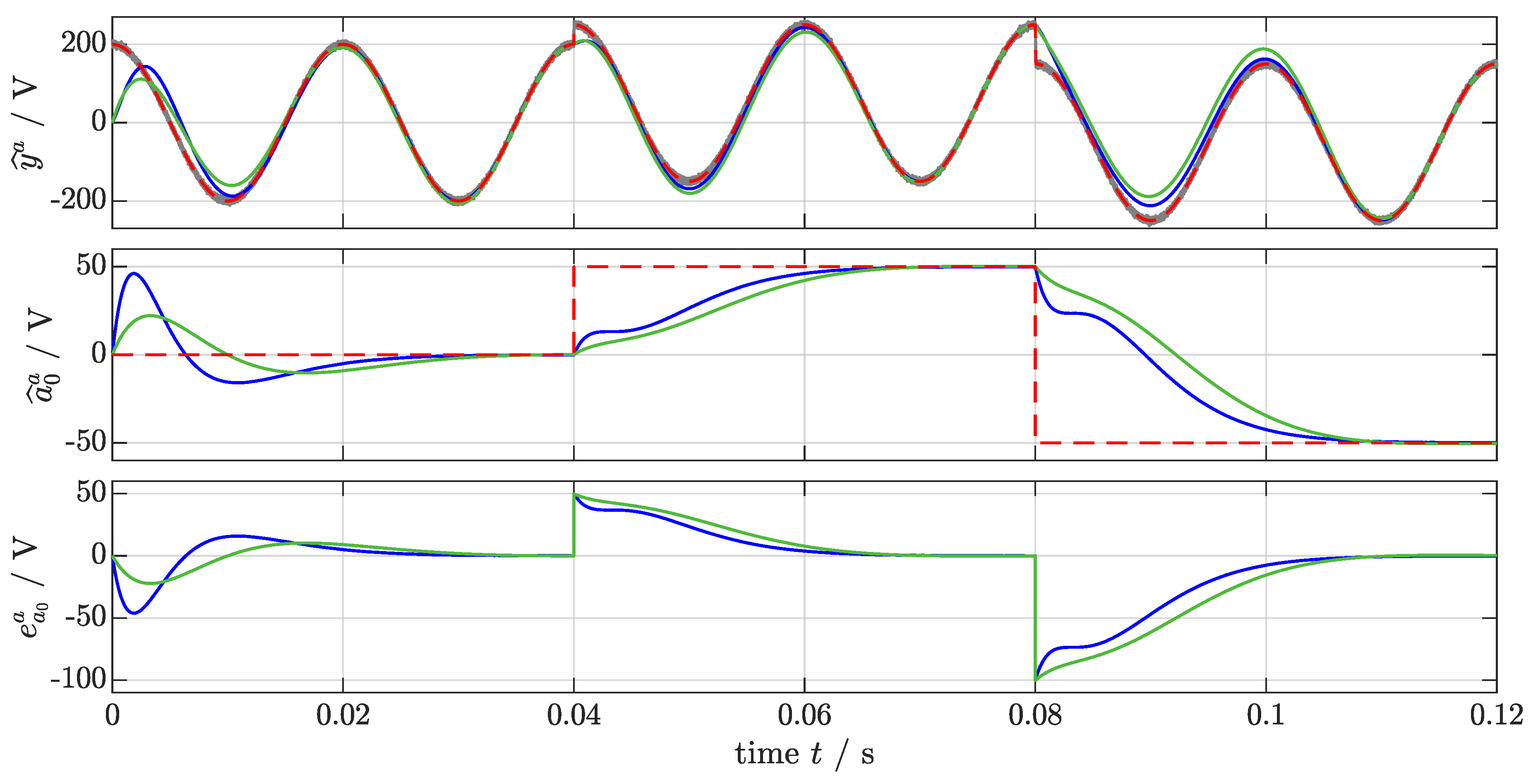
(S2)

Estimation of a fundamental, single-phase input signal $y^a$ with known and constant fundamental angular frequency and with DC-offset to (i) validate the proposed DC-offset estimation method and to compare it to the existing method [4]. The signal undergoes offset jumps of $+50 \mathrm{V}$ at t = 0.04 s and $-100 \mathrm{V}$ and at t = 0.08 s.

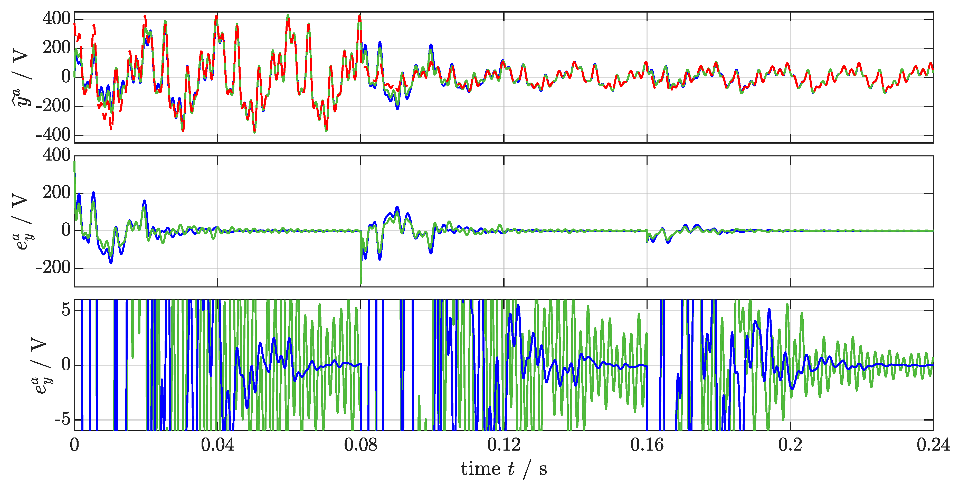
(S3)

Estimation of a single-phase input signal $y^a$ with ten harmonics, known and constant fundamental angular frequency and without DC-offset to (i) show the improved tuning method and to compare it to [13]. The signal undergoes an amplitude jump ($-75\%$) at t = 0.08 s and a phase jump ($+\frac{\pi }{3}$) at t = 0.16 s.

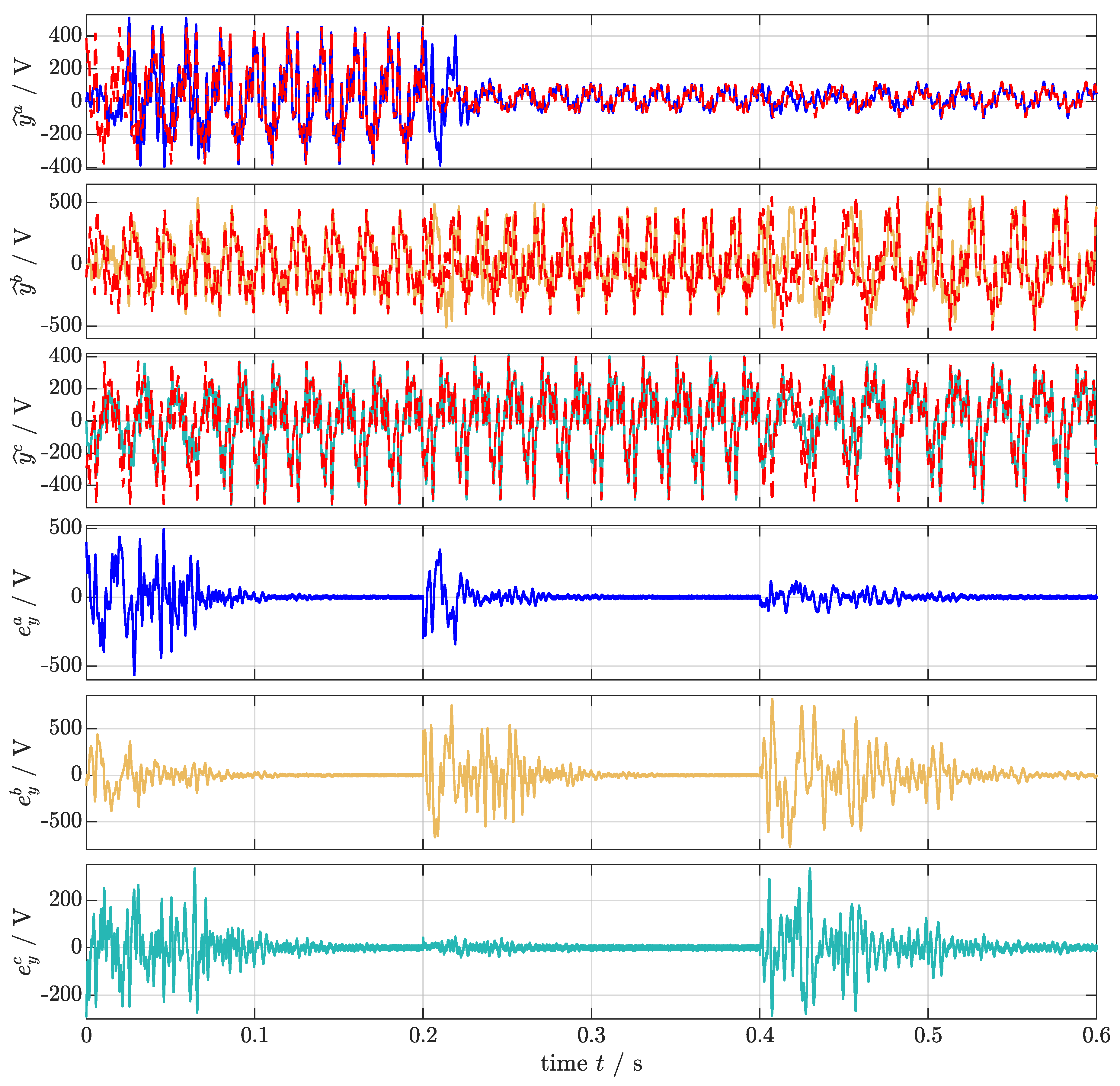
(S4)

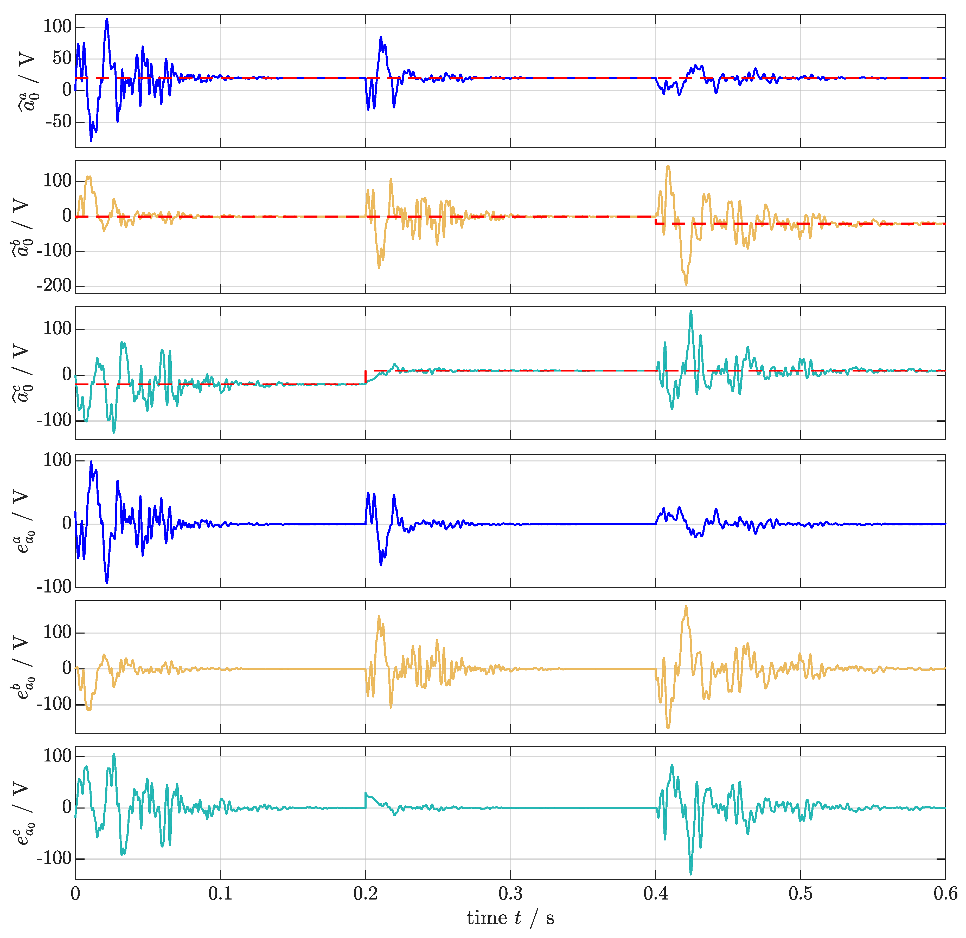
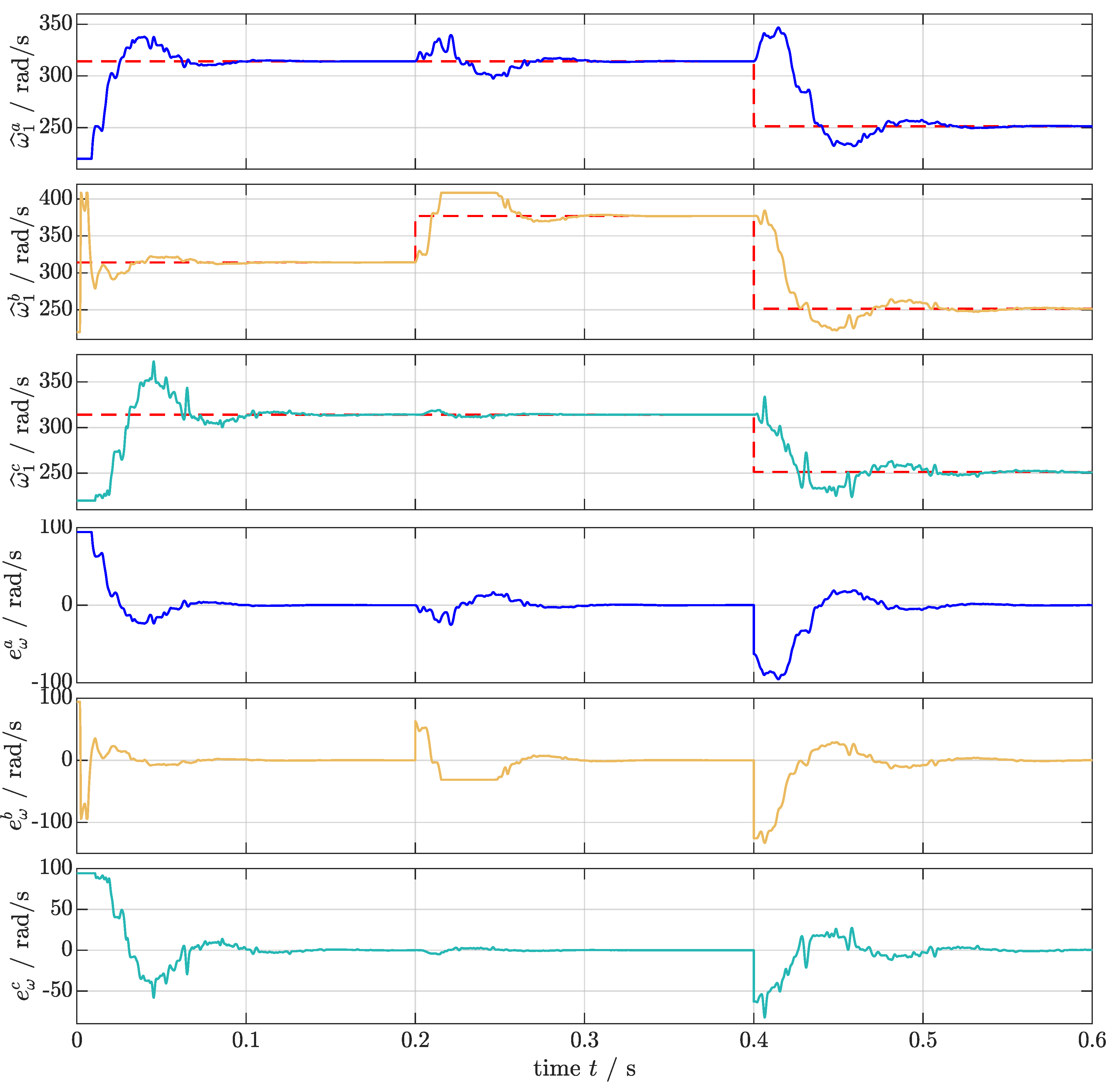
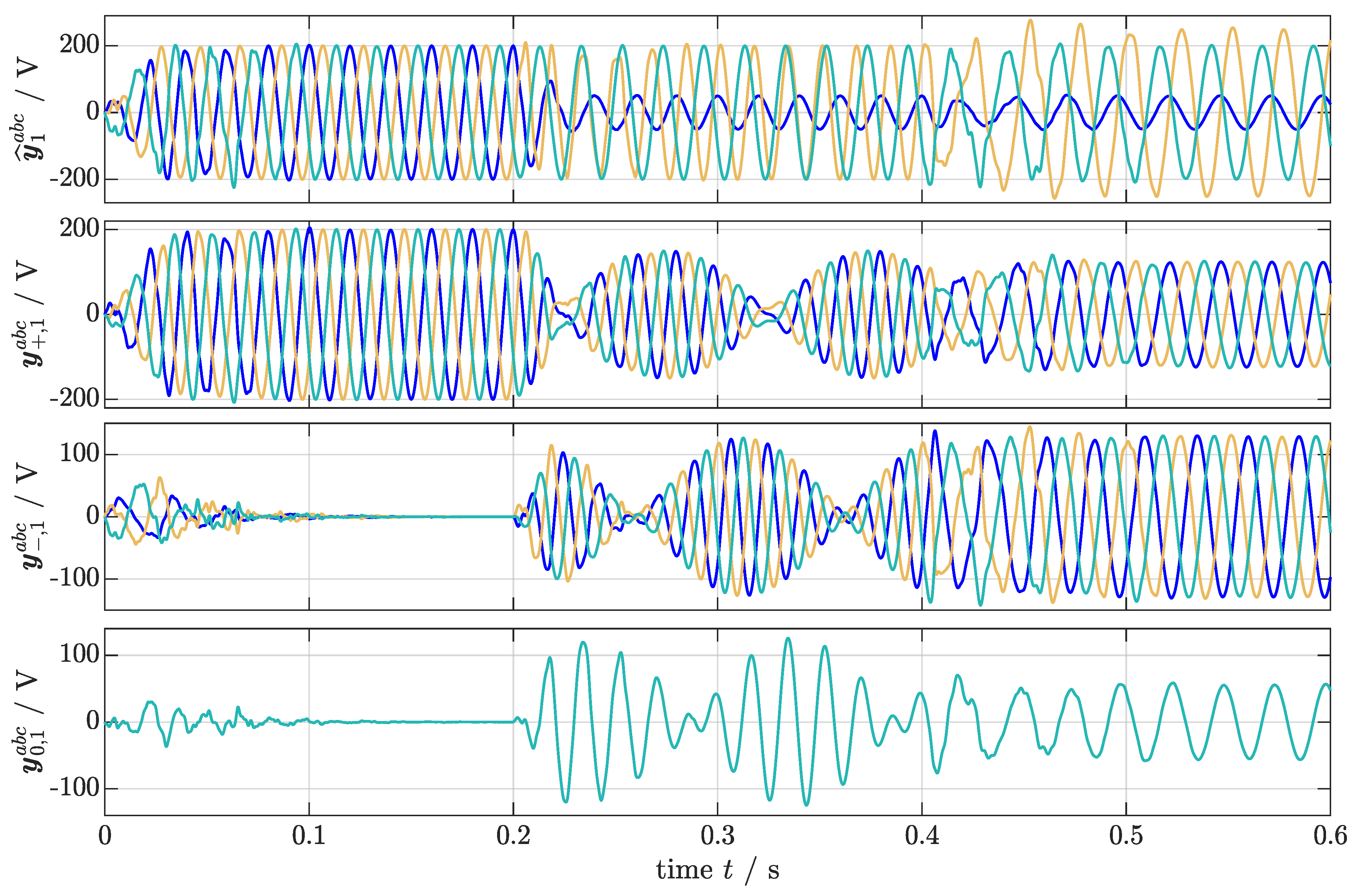
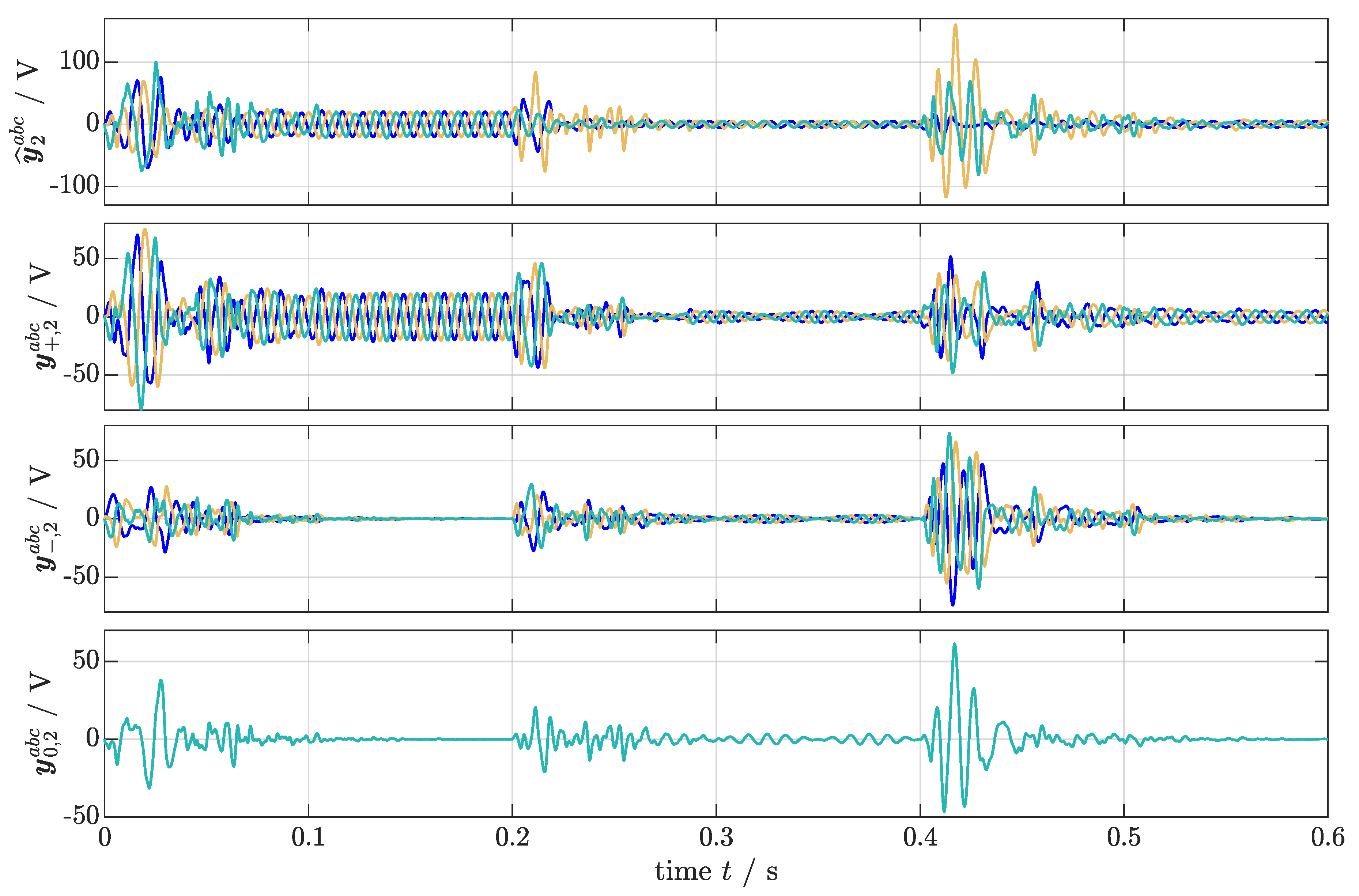
Estimation of a three-phase input signal $y^{abc}$ with ten harmonics, unknown fundamental angular frequency, and with DC-offset to verify the whole algorithm, including symmetrical components. The signals undergo (i) an amplitude jump ($-75\%$) in phase a, a phase ($+\frac{\pi }{2}\mathrm{rad}$) and frequency jump ($+2\pi 10 \mathrm{rad}/\mathrm{s}$) in phase b, and an offset jump ($+30 \mathrm{V}$) in phase c at t = 0.2 s, and (ii) a phase ($+\frac{\pi }{3}\mathrm{rad}$) and frequency jump ($-2\pi 10 \mathrm{rad}/\mathrm{s}$) in phase a, an amplitude ($+25\%$), offset ($-20 \mathrm{V}$) and frequency jump ($-2\pi 20 \mathrm{rad}/\mathrm{s}$) in phase b, and a frequency jump ($-2\pi 10 \mathrm{rad}/\mathrm{s}$) in phase c at t = 0.4 s. At $t=0 \mathrm{s}$, the three phases are balanced, and they are unbalanced at t≥ 0.2 s. Note that the second harmonic component remains balanced.

For Scenario (S1), a noisy, single-phase, offset-free input signal $y^a$ with known angular frequency ($a_1^a=200 \mathrm{V}$, $a_0^a=0 \mathrm{V}$, ${\omega }_1^a=2\pi 50 \mathrm{rad}/\mathrm{s}$) is fed into the algorithm without FLL—that is, the frequency integrator is multiplied by zero and initialized with ${\omega }_0={\omega }_1^a$. This imposes constant cutoff frequencies for the LPF and HPF, respectively; the respective APCs are constant as well. The system parameters used for this scenario are collected in Table 3.

Table 3. System parameters for Scenarios (S1), (S2), (S3), and (S4).

Scenario		(S1)	(S2)	(S3)	(S4)
Sampling time	$T_s$	$1\mathsf{\mu }\mathrm{s}$	$1\mathsf{\mu }\mathrm{s}$	$1\mathsf{\mu }\mathrm{s}$	$1\mathsf{\mu }\mathrm{s}$
Phase	p	a	a	a	a	b	c
LPF
cutoff frequency	${\omega }_{\mathrm{LPF}}^p$	$2\pi 50\frac{\mathrm{rad}}{\mathrm{s}}$	$2\pi 50\frac{\mathrm{rad}}{\mathrm{s}}$	／	$6{\widehat{\omega }}_1^a\left(t\right)$	$6{\widehat{\omega }}_1^b\left(t\right)$	$6{\widehat{\omega }}_1^c\left(t\right)$
initial value	${\xi }_{\mathrm{LPF}}^p\left(0\right)$	0$\mathrm{V}$	0$\mathrm{V}$	／	0$\mathrm{V}$	0$\mathrm{V}$	0$\mathrm{V}$
HPF
cutoff frequency	${\omega }_{\mathrm{HPF}}^p$	$4\pi 50\frac{\mathrm{rad}}{\mathrm{s}}$	$4\pi 50\frac{\mathrm{rad}}{\mathrm{s}}$	／	$8{\widehat{\omega }}_1^a\left(t\right)$	$8{\widehat{\omega }}_1^b\left(t\right)$	$8{\widehat{\omega }}_1^c\left(t\right)$
initial value	${\xi }_{\mathrm{HPF}}^p\left(0\right)$	0$\mathrm{V}$	0$\mathrm{V}$	／	0$\mathrm{V}$	0$\mathrm{V}$	0$\mathrm{V}$
SOGI
gain	${\mathit{b}}^p$	Appendix A.5	Appendix A.5	Appendix A.5	Appendix A.5	Appendix A.5	Appendix A.5
initial values	${\widehat{\mathit{x}}}_{\mathrm{HPF}}^p\left(0\right)$	${\mathbf{0}}_2{\mathrm{V}}^2$	${\mathbf{0}}_2{\mathrm{V}}^2$	${\mathbf{0}}_{20}{\mathrm{V}}^{20}$	${\mathbf{0}}_{20}{\mathrm{V}}^{20}$	${\mathbf{0}}_{20}{\mathrm{V}}^{20}$	${\mathbf{0}}_{20}{\mathrm{V}}^{20}$
FLL
gain	${\mathsf{\Gamma }}^p$	$0/\mathrm{s}$	$0/\mathrm{s}$	$0/\mathrm{s}$	$46/\mathrm{s}$	$46/\mathrm{s}$	$46/\mathrm{s}$
initial value	${\widehat{\omega }}_1^p\left(0\right)$	$2\pi 50\frac{\mathrm{rad}}{\mathrm{s}}$	$2\pi 50\frac{\mathrm{rad}}{\mathrm{s}}$	$2\pi 50\frac{\mathrm{rad}}{\mathrm{s}}$	$200\frac{\mathrm{rad}}{\mathrm{s}}$	$200\frac{\mathrm{rad}}{\mathrm{s}}$	$200\frac{\mathrm{rad}}{\mathrm{s}}$
GN
lower amplitude	${\underline{a}}_1^p$	／	／	／	0.01 V2	0.01 V2	0.01 V2
OS
lower frequency	${\underline{\omega }}^p$	／	／	／	$2\pi 35\frac{\mathrm{rad}}{\mathrm{s}}$	$2\pi 35\frac{\mathrm{rad}}{\mathrm{s}}$	$2\pi 35\frac{\mathrm{rad}}{\mathrm{s}}$
upper frequency	${\overline{\omega }}^p$	／	／	／	$2\pi 65\frac{\mathrm{rad}}{\mathrm{s}}$	$2\pi 65\frac{\mathrm{rad}}{\mathrm{s}}$	$2\pi 65\frac{\mathrm{rad}}{\mathrm{s}}$
Reference model		／	[4]	[13]	／	／	／
SOGI gain	${\mathit{b}}^p$	／	${\left(\begin{array}{cc}1.28& 0\end{array}\right)}^{\top }$	${\mathit{c}}_y$	／	／	／
DC gain	$k_{\mathrm{dc}}^p$	／	0.26	／	／	／	／
initial values	${\widehat{\mathit{x}}}^p\left(0\right)$	／	${\mathbf{0}}_3{\mathrm{V}}^3$	${\mathbf{0}}_{20}{\mathrm{V}}^{20}$	／	／	／

Considering Scenario (S2), a noisy, single-phase input signal $y^a$ with known angular frequency ($a_1^a=200 \mathrm{V}$, ${\omega }_1^a=2\pi 50 \mathrm{rad}/\mathrm{s}$) and step-like changes in the DC-offset is fed (i) to the proposed algorithm and (ii) to a SOGI capable of estimating offsets taken from [4]. For both models, the FLL is turned off as in (S1). The system parameters for this scenario are shown in Table 3.

Scenario (S3) uses a noise-free, single-phase input signal with ten harmonics, known fundamental angular frequency, and without DC-offset, but does use step-like changes in amplitude and angle to compare the proposed tuning method to standard tunings. As a reference, model and tuning from [13] are used. To focus only on the impact of the tuning, LPF, HPF, and FLL are disabled (but still implemented). The system parameters are listed in Table 3, as well as the signal variables in Table 4 (only phase a is used).

Table 4. Signal variables for Scenarios (S3) and (S4).

$\mathit{\nu }$	0	1	2	3	4	5	6	7	8	9	10
$0\mathrm{s}\le$t < 0.2 s
$a_{\nu }^a$	20	200	20	80	120	40	80	60	20	0	100
${\varphi }_{\nu }^a(t=0\mathrm{s})/\mathrm{rad}$		0	$\frac{2\pi }{3}$	$\frac{\pi }{6}$	$\frac{7\pi }{4}$	$\frac{5\pi }{3}$	$\frac{5\pi }{6}$	0	$\frac{\pi }{4}$	$\frac{\pi }{3}$	$\frac{\pi }{2}$
${\omega }_1^a/\mathrm{rad}/\mathrm{s}$	$2\pi 50$
$a_{\nu }^b$	0	200	20	80	120	40	80	60	20	0	100
${\varphi }_{\nu }^b(t=0\mathrm{s})/\mathrm{rad}$		$\frac{4\pi }{3}$	0	$\frac{3\pi }{2}$	$\frac{13\pi }{12}$	$\pi$	$\frac{\pi }{6}$	$\frac{4\pi }{3}$	$\frac{19\pi }{12}$	$\frac{5\pi }{3}$	$\frac{11\pi }{6}$
${\omega }_1^b/\mathrm{rad}/\mathrm{s}$	$2\pi 50$
$a_{\nu }^c$	$-20$	200	20	80	120	40	80	60	20	0	100
${\varphi }_{\nu }^c(t=0\mathrm{s})/\mathrm{rad}$		$\frac{2\pi }{3}$	$\frac{4\pi }{3}$	$\frac{5\pi }{6}$	$\frac{5\pi }{12}$	$\frac{\pi }{3}$	$\frac{3\pi }{2}$	$\frac{2\pi }{3}$	$\frac{11\pi }{12}$	$\pi$	$\frac{7\pi }{6}$
${\omega }_1^c/\mathrm{rad}/\mathrm{s}$	$2\pi 50$
0.2 s $\le t$ < 0.4 s
$a_{\nu }^a$	20	50	5	0	30	10	20	15	5	0	25
${\varphi }_{\nu }^a(t=0.2$s$)/\mathrm{rad}$		0	$\frac{2\pi }{3}$	$\frac{\pi }{6}$	$\frac{7\pi }{4}$	$\frac{5\pi }{3}$	$\frac{5\pi }{6}$	0	$\frac{\pi }{4}$	$\frac{\pi }{3}$	$\frac{\pi }{2}$
${\omega }_1^a/\mathrm{rad}/\mathrm{s}$	$2\pi 50$
$a_{\nu }^b$	0	200	5	80	120	40	80	60	20	0	100
${\varphi }_{\nu }^b(t=0.2$s$)/\mathrm{rad}$		$\frac{11\pi }{6}$	0	0	$\frac{19\pi }{12}$	$\frac{3\pi }{2}$	$\frac{2\pi }{3}$	$\frac{11\pi }{6}$	$\frac{\pi }{12}$	$\frac{\pi }{6}$	$\frac{\pi }{3}$
${\omega }_1^b/\mathrm{rad}/\mathrm{s}$	$2\pi 60$
$a_{\nu }^c$	10	200	5	80	120	40	80	60	20	0	100
${\varphi }_{\nu }^c(t=0.2$s$)/\mathrm{rad}$		$\frac{2\pi }{3}$	$\frac{4\pi }{3}$	$\frac{5\pi }{6}$	$\frac{5\pi }{12}$	$\frac{\pi }{3}$	$\frac{3\pi }{2}$	$\frac{2\pi }{3}$	$\frac{11\pi }{12}$	$\pi$	$\frac{7\pi }{6}$
${\omega }_1^c/\mathrm{rad}/\mathrm{s}$	$2\pi 50$
0.4 s $\le t\le$ 0.6 s
$a_{\nu }^a$	20	50	5	0	30	10	20	15	5	0	25
${\varphi }_{\nu }^a(t=0.4$s$)/\mathrm{rad}$		$\frac{\pi }{3}$	$\pi$	$\frac{\pi }{2}$	$\frac{\pi }{12}$	0	$\frac{7\pi }{6}$	$\frac{\pi }{3}$	$\frac{7\pi }{12}$	$\frac{2\pi }{3}$	$\frac{5\pi }{6}$
${\omega }_1^a/\mathrm{rad}/\mathrm{s}$	$2\pi 40$
$a_{\nu }^b$	$-20$	250	5	100	150	50	100	75	25	0	125
${\varphi }_{\nu }^b(t=0.4$s$)/\mathrm{rad}$		$\frac{11\pi }{6}$	$\frac{\pi }{3}$	0	$\frac{19\pi }{12}$	$\frac{3\pi }{2}$	$\frac{2\pi }{3}$	$\frac{11\pi }{6}$	$\frac{\pi }{12}$	$\frac{\pi }{6}$	$\frac{\pi }{3}$
${\omega }_1^b/\mathrm{rad}/\mathrm{s}$	$2\pi 40$
$a_{\nu }^c$	10	200	5	80	120	40	80	60	20	0	100
${\varphi }_{\nu }^c(t=0.4$s$)/\mathrm{rad}$		$\frac{2\pi }{3}$	$\frac{5\pi }{3}$	$\frac{5\pi }{6}$	$\frac{5\pi }{12}$	$\frac{\pi }{3}$	$\frac{3\pi }{2}$	$\pi$	$\frac{11\pi }{12}$	$\pi$	$\frac{7\pi }{6}$
${\omega }_1^c/\mathrm{rad}/\mathrm{s}$	$2\pi 40$

For Scenario (S4), noisy and biased three-phase signals $y^{abc}$ with ten harmonics each are used for algorithm verification. The amplitudes, phases, offsets, and frequencies of the harmonic components have step-like changes in amplitudes, phase angles, frequencies, and DC-offsets. In this scenario, the FLL is turned on (one for each phase) and its estimated frequency is used for the respective LPF, HPF, and SOGIs (which implies constant APC matrices). The filters, SOGIs, and FLLs are tuned identically for all phases. All parameters have been collected and shown in Table 3, and all signal variables in Table 4.

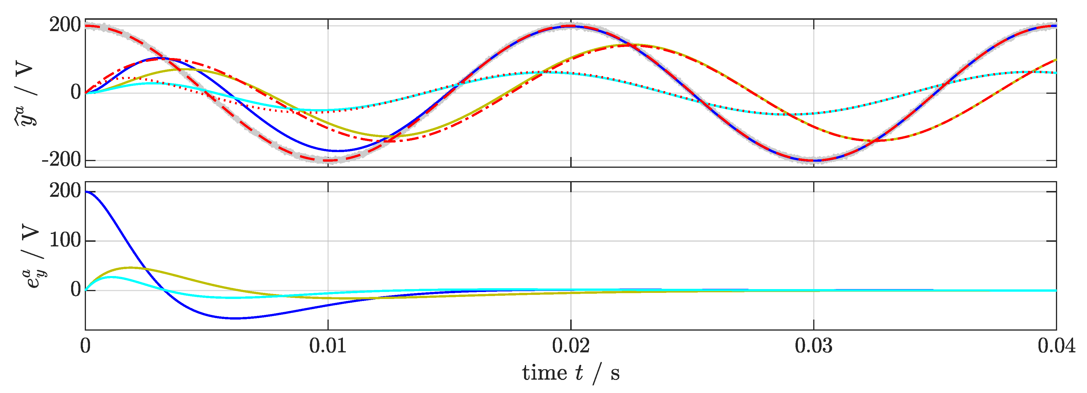
3.1. Discussion of the Simulation Results of Scenario (S1)

The scope of Scenario (S1) was to show the influence of Low- and High-Pass Filters and their respective Amplitude Phase Corrections; hence, the SOGI was driven without FLL. The SOGI was tuned such that the fastest possible time response could be achieved, and the pre-filters acted as a band-pass filter (see Table 3).

Figure 5 shows things besides the noise-free input signal $y_{\mathrm{won}}^a$ (), the noisy input signal $y^a$ (), which is damped and shifted due to the LPF (), and HPF (). The resulting signal $y_{\mathrm{HPF}}^a$ was analyzed by the SOGI, whose in-phase output ${\widehat{y}}_{\mathrm{HPF}}^a$ (), the reconstructed in-phase outputs of the APC${}_{\mathrm{HPF}}$${\widehat{y}}_{\mathrm{LPF}}^a$ (), and APC${}_{\mathrm{LPF}}$${\widehat{y}}^a$ (), respectively, are shown. The APCs reconstruct the original input signal correctly, which can be seen in the estimation errors $e_y^a:=y_{\mathrm{won}}^a-{\widehat{y}}^a$ (), $e_{\mathrm{LPF},y}^a:=y_{\mathrm{LPF}}^a-{\widehat{y}}_{\mathrm{LPF}}^a$ (), and $e_{\mathrm{HPF},y}^a:=y_{\mathrm{HPF}}^a-{\widehat{y}}_{\mathrm{HPF}}^a$ (), which tend toward zero within $20\mathrm{m}\mathrm{s}$.

Figure 5. Simulation results for Scenario (S1): Noise-free input ($y_{\mathrm{won}}^a$: ), noisy input ($y^a$: ), LPF ($y_{\mathrm{LPF}}^a$: ), and HPF ($y_{\mathrm{HPF}}^a$: ) signals, its estimates, and respective errors (${\widehat{y}}^a$, $e_y^a$: ; ${\widehat{y}}_{\mathrm{LPF}}^a$, $e_{\mathrm{LPF},y}^a$: ; and ${\widehat{y}}_{\mathrm{HPF}}^a$, $e_{\mathrm{HPF},y}^a$: ).

3.2. Discussion of the Simulation Results of Scenario (S2)

In Scenario (S2), the proposed DC-offset detection method was compared to an existing method [4] to obtain a better insight into the estimation performance, and the FLL is turned off in both models. The pre-filters and SOGI are tuned as described in Table 3; the tuning for the referenced SOGI is taken from [4]. The input signal undergoes step-like changes in the DC-offset, as described above.

In Figure 6, the first, second, and third subplots show the noise-free input signal $y_{\mathrm{won}}^a$ (), the noisy input signal $y^a$ (), & its estimates ${\widehat{y}}^a$ (this paper: , [4]: ), the DC-offset $a_0^a$ & and its estimates ${\widehat{a}}_0^a$, and the error in DC-offset estimation $e_{a_0}^a:=a_0^a-{\widehat{a}}_0^a$, respectively. The proposed method estimates the input signal and the DC-offset asymptotically. Moreover, the DC-offset estimation of the proposed method is faster than the DC-SOGI, but is clearly still limited due to the limited time response of the SOGI. The time response can be made faster by tuning the filters accordingly, which, on the other hand, leads to larger overshoots.

Figure 6. Simulation results for Scenario (S2): Noisy input $y^a$ (), noise-free input $y_{\mathrm{won}}^a$, and DC-offset $a_0^a$ (), its estimates ${\widehat{y}}^a$ & ${\widehat{a}}_0^a$ and DC-offset estimation error $e_{a_0}^a$ (this paper: , [4]: ).

3.3. Discussion of the Simulation Results of Scenario (S3)

Scenario (S3) compares the proposed tuning method to the standard tuning [13]. To be able to compare the tuning methods, the model used for validation was reduced to its basics—that is, without pre-filters (and APCs) and FLL; the respective parameters have been collected and shown in Table 3. The input specifications (only phase a) are described in Table 4.

Figure 7 shows the input signal $y^a$ (), and its estimate ${\widehat{y}}^a$ with the proposed tuning () and the standard tuning () in the first subplot; the second subplot shows the respective errors $e_y^a:=y^a-{\widehat{y}}^a$, which are shown again in a close-up in the third subplot. Both methods are able to track the input signal asymptotically. However, by using the proposed tuning, the settling time reduces to $70\mathrm{m}\mathrm{s}$; where in contrast, the standard tuning does not settle down satisfactory in the time-frames shown, and is much more turbulent. On the other hand, this faster time response comes at the cost of (slightly) higher overshooting (see, e.g., $0 \mathrm{s}$$\le t$ < 0.02 s).

Figure 7. Simulation results for Scenario (S3): Input signal $y^a$ (), its estimates ${\widehat{y}}^a$, and estimation errors $e_y^a$ (this paper: , [13]: ).

3.4. Discussion of the Simulation Results of Scenario (S4)

In Scenario (S4), the proposed overall estimation method (as in Figure 1) is investigated. Each phase is filtered by a bandpass whose cut-off frequencies depend on the estimated fundamental angular frequencies of the respective phases. Therefore, each phase has a separate frequency detection. The SOGIs and FLL-GN-OSs are tuned identically (see Table 3). As a test signal, a three-phase input with differing step-like changes in each variable in each phase is used (see Table 4).

In subplots 1 to 3 of Figure 8, the three-phase, noise-free input signals $y_{\mathrm{won}}^a$, $y_{\mathrm{won}}^b$ & $y_{\mathrm{won}}^c$ () (but not the noisy signals $y^a$, $y^b$ or $y^c$) and its estimates ${\widehat{y}}^a$ (), ${\widehat{y}}^b$ () & ${\widehat{y}}^c$ () are shown, whereas in the subplots 4 to 6, the estimation errors $e_y^a:=y^a-{\widehat{y}}^a$, $e_y^b:=y^b-{\widehat{y}}^b$ and $e_y^c:=y^c-{\widehat{y}}^c$ are depicted. All SOGIs estimate the input signal properly.

Figure 8. Simulation results for Scenario (S4): Inputs $y_{\mathrm{won}}^a$, $y_{\mathrm{won}}^b$ & $y_{\mathrm{won}}^c$ (), its estimates ${\widehat{y}}^a$, ${\widehat{y}}^b$ & ${\widehat{y}}^c$ and errors $e_y^a$, $e_y^b$ & $e_y^c$ (phase a: ; phase b: ; phase c: ).

Figure 9 shows the DC-offsets $a_0^a$, $a_0^b$ & $a_0^c$ (), its estimates ${\widehat{a}}_0^a$, ${\widehat{a}}_0^b$ & ${\widehat{a}}_0^c$, and errors $e_{a_0}^a:=a_0^a-{\widehat{a}}_0^a$, $e_{a_0}^b:=a_0^b-{\widehat{a}}_0^b$ & $e_{a_0}^c:=a_0^c-{\widehat{a}}_0^c$ (phase a: ; phase b: ; phase c: ) in subplots 1 to 6, respectively. The combination of HPF and APC${}_{\mathrm{HPF}}$ estimates the DC-offsets correctly.

Figure 9. Simulation results for Scenario (S4): DC-offset $a_0^a$, $a_0^b$ & $a_0^c$ (), its estimates ${\widehat{a}}_0^a$, ${\widehat{a}}_0^b$ & ${\widehat{a}}_0^c$, and errors $e_{a_0}^a$, $e_{a_0}^b$ & $e_{a_0}^c$ (phase a: ; phase b: ; phase c: ).

In Figure 10, the fundamental angular frequencies ${\omega }_1^a$, ${\omega }_1^b$ & ${\omega }_1^c$ () and its estimates ${\widehat{\omega }}_1^a$, ${\widehat{\omega }}_1^b$ & ${\widehat{\omega }}_1^c$ (phase a: ; phase b: ; phase c: ) are shown in the first three subplots; in the last three subplots, the respective errors $e_{\omega }^a:={\omega }_1^a-{\widehat{\omega }}_1^a$, $e_{\omega }^b:={\omega }_1^b-{\widehat{\omega }}_1^b$ & $e_{\omega }^c:={\omega }_1^c-{\widehat{\omega }}_1^c$ (phase a: ; phase b: ; phase c: ) are illustrated. The FLLs, in combination with the GN and OS, estimate the fundamental angular frequencies correctly. However, clearly, comparing Scenario (S4) to (S3), the FLLs slow down the overall system; an overall estimation is achieved within 0.16 s or less. The proposed frequency limitation (OS) enforces the frequency estimation to stay within the defined band (despite the initial values), which prevents overshooting (see ${\widehat{\omega }}_1^b$ at $t\approx$ 0.23 s).

Figure 10. Simulation results for Scenario (S4): Fundamental angular frequency ${\omega }_1^a$, ${\omega }_1^b$ & ${\omega }_1^c$ (), its estimates ${\widehat{\omega }}_1^a$, ${\widehat{\omega }}_1^b$ & ${\widehat{\omega }}_1^c$, and errors $e_{\omega }^a$, $e_{\omega }^b$ & $e_{\omega }^c$ (phase a: ; phase b: ; phase c: ).

Considering the effects of the variable jumps to the overall system,

• The offset jump ($+30 \mathrm{V}$ at t = 0.2 s in phase c) has almost no influence on the overall system; the changed input is estimated in about 0.03 s;
• The amplitude jump ($-75\%$ at t = 0.2 s in phase a) causes moderate system errors; the system takes approximately 0.08 s to settle down again; and
• The frequency jump ($-2\pi 10 \mathrm{rad}/\mathrm{s}$ at t = 0.4 s in phase c) severely excites the settled system; it requires 0.16 s to settle down.

Figure 11 shows, from top to bottom, the estimated fundamental in-phase signals ${\widehat{\mathit{y}}}_1^{abc}$, and from it, the calculated positive- ${\widehat{\mathit{y}}}_{+,1}^{abc}$, negative- ${\widehat{\mathit{y}}}_{-,1}^{abc}$ and zero-sequence ${\widehat{\mathit{y}}}_{0,1}^{abc}$ (phase a: ; phase b: ; phase c: ). In general, the positive-, negative-, and zero-sequence only shows in the steady-state. In the first time-frame, ($0 \mathrm{s}\le t<$ 0.2 s), the fundamental component is balanced, so the symmetrical component calculation only shows the positive sequence. In the second time-frame (0.2 s $\le t<$ 0.4 s), the frequencies are not identical, so the symmetrical components cannot be calculated anymore; in fact, the positive-, negative-, and zero-sequences are enclosed by an oscillating hull, wherein each of the phases has the same frequency, which is unequal to the true signal frequencies. In the last time-frame (0.4 s $\le t\le$ 0.6 s), the frequencies are identical, and the harmonic sequence detection works properly again. As defined, the fundamental component is unbalanced, which finds itself in the presence of a negative and zero sequence.

Figure 11. Simulation results for Scenario (S4): Estimated in-phase signals ${\widehat{\mathit{y}}}_1^{abc}$, calculated positive- ${\mathit{y}}_{+,1}^{abc}$, negative- ${\mathit{y}}_{-,1}^{abc}$ and zero-sequence ${\mathit{y}}_{0,1}^{abc}$ of the fundamental component (phase a: ; phase b: ; phase c: ).

In Figure 12, the estimated second harmonic in-phase signals ${\widehat{\mathit{y}}}_2^{abc}$ and its positive- ${\widehat{\mathit{y}}}_{+,2}^{abc}$, negative- ${\widehat{\mathit{y}}}_{-,2}^{abc}$, and zero-sequence ${\widehat{\mathit{y}}}_{0,2}^{abc}$ are shown from top to bottom, respectively (phase a: ; phase b: ; phase c: ). Since the second harmonic component is balanced for all time steps, the negative and zero sequence only show in the time-frame with differing frequencies. Referring to this time-frame 0.2 s $\le t$ < 0.4 s, the sequence signals and the hull oscillate with double frequency with respect to the fundamental component.

Figure 12. Simulation results for Scenario (S4): Estimated in-phase signals ${\widehat{\mathit{y}}}_2^{abc}$, calculated positive- ${\mathit{y}}_{+,2}^{abc}$, negative- ${\mathit{y}}_{-,2}^{abc}$ and zero-sequence ${\mathit{y}}_{0,2}^{abc}$ of the second harmonic component (phase a: ; phase b: ; phase c: ).

4. Conclusions and Outlook

This paper presented a unified method for online detection of symmetrical components. The key tools herein were parallelized Second-Order Generalized Integrators (SOGIs) to obtain estimates of direct and quadrature signals of the harmonic components, for which a new tuning method was proposed. Frequency estimation was achieved by a Frequency Locked Loop (FLL) with Gain Normalization (GN) which was extended by an Output Saturation (OS) to ensure stability of the overall system. DC-offset detection was applied by a combination of High-Pass Filter (HPF) and HPF-Amplitude Phase Correction (APC${}_{\mathrm{HPF}}$); additional noise filtering was done by a Low-Pass Filter (LPF) with respective APC${}_{\mathrm{LPF}}$. Finally, a Harmonic Sequence Detection (HSD) for the calculation of the symmetrical components of each harmonic was incorporated. For the overall system, a stability proof was carried out; only for the FLL was a convergence proof not found. The proposed DC-offset detection method allowed for an easy tuning of the system in contrast to existing methods, where, to the best knowledge of the authors, no system capable of estimating harmonics and offset has yet been investigated, nor has stability for such a system been proven. The modification in the SOGI tuning achieved a faster system response with only a moderate increase of overshooting, leading to a shorter overall settling time. The combination of filters and respective APCs allowed noise reduction without undesired damping and phase lag of the input signal.

Future work will focus on the FLL, which remains the bottleneck of the overall system since it significantly reduces the overall settling time.

Appendix A.1. Hurwitz Stability

Theorem A1 (Hurwitz system matrix).

Let $p\in \left\{a,b,c\right\}$, ${\mathbb{H}}_n$ as in (3) and ${\mathit{A}}^p$ as in (13). Then, if and only if $k_i^p>0,i\in \left\{1,\dots ,n\right\}$, the system matrix ${\mathit{A}}^p$ is a Hurwitz matrix and all its eigenvalues have negative real part—that is, 

$$\forall k_i^p>0,i\in \left\{1,\dots ,n\right\}:\Re \left(\lambda \right)<0,\lambda \in \left\{\left.s\in \mathbb{C}\right|{\chi }_{{\mathit{A}}^p}\left(s\right):=det(s{\mathit{I}}_{2n}-{\mathit{A}}^p)=0\right\}.$$

Figure A1. Block diagram of (13) using transfer functions.

Proof. 

First note that, for constant ${\widehat{\omega }}_1^p>0$, the system (13) can be represented by transfer functions as depicted in Figure A1.

Hence, each sub-transfer function ${\mathcal{V}}_i^p\left(s\right):=\frac{{\widehat{y}}_i^p\left(s\right)}{y^p\left(s\right)}$ with $i\in \{1,\cdots ,n\}$ is given by

$${\displaystyle {\mathcal{V}}_i^p\left(s\right)=\frac{\frac{{\nu }_i{k}_i^p{\widehat{\omega }}_1^{p}s}{s^2+{\left({\nu }_i{\widehat{\omega }}_1^p\right)}^2}}{1+{\displaystyle \sum _{j=1}^n}\frac{{\nu }_j{k}_j^p{\widehat{\omega }}_1^{p}s}{s^2+{\left({\nu }_j{\widehat{\omega }}_1^p\right)}^2}}=\frac{{\nu }_i{k}_i^p{\widehat{\omega }}_1^{p}s{\displaystyle \prod _{\begin{array}{c}j=1\\ j\ne i\end{array}}^n}\left(s^2+{\left({\nu }_j{\widehat{\omega }}_1^p\right)}^2\right)}{{\displaystyle \prod _{j=1}^n}\left(s^2+{\left({\nu }_j{\widehat{\omega }}_1^p\right)}^2\right)+{\displaystyle \sum _{j=1}^n}{\nu }_j{k}_j^p{\widehat{\omega }}_1^{p}s{\displaystyle \prod _{\begin{array}{c}l=1\\ l\ne j\end{array}}^n}\left(s^2+{\left({\nu }_l{\widehat{\omega }}_1^p\right)}^2\right)}}$$

(A1)

and the characteristic polynomial of the overall system in Figure A1 is given by the denominator of (A1), i.e.,

$$\begin{array}{ccc}\hfill \chi \left(s\right)& =& {\displaystyle \prod _{j=1}^n}\left(s^2+{\left({\nu }_j{\widehat{\omega }}_1^p\right)}^2\right)+{\displaystyle \sum _{j=1}^n}{\nu }_j{k}_j^p{\widehat{\omega }}_1^{p}s{\displaystyle \prod _{\begin{array}{c}l=1\\ l\ne j\end{array}}^n}\left(s^2+{\left({\nu }_l{\widehat{\omega }}_1^p\right)}^2\right)\hfill \end{array}$$

$$\begin{array}{ccc}\hfill & \stackrel{\widehat{s}:=\frac{s}{{\widehat{\omega }}_1^p}}{=}& {({\widehat{\omega }}_1^p)}^{2n}\left[\underset{=:{\chi }_{{\mathit{A}}^p}^e\left(\widehat{s}\right)}{\underbrace{{\displaystyle \prod _{\begin{array}{c}j=1\end{array}}^n}\left({\widehat{s}}^2+{\nu }_j^2\right)}}+\underset{=:{\chi }_{{\mathit{A}}^p}^o\left(\widehat{s}\right)}{\underbrace{{\displaystyle \sum _{j=1}^n}{\nu }_j{k}_j^p\widehat{s}\prod _{\begin{array}{c}l=1\\ l\ne j\end{array}}^n\left({\widehat{s}}^2+{\nu }_l^2\right)}}\right]\hfill \end{array}$$

(A2)

$$\begin{array}{cc}=& {\left({\widehat{\omega }}_1^p\right)}^{2n}{\chi }_{{\mathit{A}}^p}\left(\widehat{s}\right)=det\left(s{\mathit{I}}_{2n}-{\widehat{\omega }}_1^p{\mathit{A}}^p\right).\hfill \end{array}$$

(A3)

Note that the characteristic polynomial ${\chi }_{{\mathit{A}}^p}\left(\widehat{s}\right)={\chi }_{{\mathit{A}}^p}^e\left(\widehat{s}\right)+{\chi }_{{\mathit{A}}^p}^o\left(\widehat{s}\right)$ can be split in even ${\chi }_{{\mathit{A}}^p}^e\left(\widehat{s}\right)$ and odd ${\chi }_{{\mathit{A}}^p}^o\left(\widehat{s}\right)$ polynomials (having even and odd order, resp.). Now, the system matrix ${\mathit{A}}^p$ is a Hurwitz matrix if and only if the following three conditions hold ([44], Fact 11.17.6): (i) all coefficients of ${\chi }_{{\mathit{A}}^p}\left(\widehat{s}\right)$ are positive, (ii) for all $s^e\in \left\{\left.s\in \mathbb{C}\right|{\chi }_{{\mathit{A}}^p}^e\left(s\right)=0\right\}$ and $s^o\in \left\{\left.s\in \mathbb{C}\right|{\chi }_{{\mathit{A}}^p}^o\left(s\right)=0\right\}$, we have $\Re \left(s^e\right)=0$ and $\Re \left(s^o\right)=0$, resp., and (iii) the roots are interlaced—that is, $\Im \left(s_1^e\right)<\Im \left(s_1^o\right)<\Im \left(s_2^e\right)<\dots <\Im \left(s_{2n-1}^e\right)<\Im \left(s_{2n-1}^o\right)<\Im \left(s_{2n}^e\right)$.

To prove this, all three conditions are shown: It is easy to see that, for all $k_i^p>0$ and since ${\nu }_i>0$ for all $i\in \{1,\cdots ,n\}$, the coefficients are products and sums of positive constants. Hence, all coefficients of the characteristic polynomial ${\chi }_{{\mathit{A}}^p}\left(\widehat{s}\right)$ are positive which shows that condition (i) is satisfied.

Next conditions (ii) and (iii) are shown. Note that, with j being the imaginary unit, the roots of even polynomial ${\chi }_{{\mathit{A}}^p}^e\left(s\right)$ are given by 

$$\forall i\in \{1,\cdots ,n\}:s_{i_{1,2}}^e=\pm j{\nu }_i⟹\Re \left(s_{i_{1,2}}^e\right)=0,$$

Except $s_0^o=0$ (clearly, with $\Re \left(s_0^o\right)=0$), the other roots of odd polynomial ${\chi }_{{\mathit{A}}^p}^o\left(s\right)$ cannot be computed analytically but can be estimated using the intermediate value theorem. Therefore, consider two consecutive positive roots $s_x^e$ and $s_y^e$, $x,y\in \left\{1,\dots ,n\right\}$ of even polynomial ${\chi }_{{\mathit{A}}^p}^e\left(s\right)$ and insert those into odd polynomial ${\chi }_{{\mathit{A}}^p}^o\left(s\right)$ which yields

$$\begin{array}{ccc}\hfill {\chi }_{{\mathit{A}}^p}^o\left(s_x^e\right)& =& j{\nu }_x^2{k}_x^p\underset{=:{\mathsf{\Lambda }}_x}{\underbrace{\left({\nu }_1^2-{\nu }_x^2\right)\dots \left({\nu }_{x-1}^2-{\nu }_x^2\right)}}\left({\nu }_y^2-{\nu }_x^2\right)\underset{=:{\mathsf{\Gamma }}_x}{\underbrace{\left({\nu }_{y+1}^2-{\nu }_x^2\right)\dots \left({\nu }_n^2-{\nu }_x^2\right)}}\hfill \\ \hfill {\chi }_{{\mathit{A}}^p}^o\left(s_y^e\right)& =& j{\nu }_y^2{k}_y^p\underset{=:{\mathsf{\Lambda }}_y}{\underbrace{\left({\nu }_1^2-{\nu }_y^2\right)\dots \left({\nu }_{x-1}^2-{\nu }_y^2\right)}}\left({\nu }_x^2-{\nu }_y^2\right)\underset{=:{\mathsf{\Gamma }}_y}{\underbrace{\left({\nu }_{y+1}^2-{\nu }_y^2\right)\dots \left({\nu }_n^2-{\nu }_y^2\right)}}.\hfill \end{array}$$

(A4)

Now, according to the intermediate value theorem, a continuous function f has at least one root in the open interval $\left(a,b\right)$ if $f\left(a\right)$ and $f\left(b\right)$ have opposite signs ([45], p. 132). Since the terms ${\mathsf{\Lambda }}_x$, ${\mathsf{\Lambda }}_y$, ${\mathsf{\Gamma }}_x$ and ${\mathsf{\Gamma }}_y$ contain an equal amount of positive and negative factors, only for $sign\left(k_x^p\right)=sign\left(k_y^p\right)$ it follows that $sign\left({\chi }_{{\mathit{A}}^p}^o\left(s_x^e\right)\right)=-sign\left({\chi }_{{\mathit{A}}^p}^o\left(s_y^e\right)\right)$ and furthermore $\exists s^o\in \left(s_x^e,s_y^e\right)\mathrm{s}.\mathrm{t}.{\chi }_{{\mathit{A}}^p}^o\left(s^o\right)=0$. Hence, it holds $\Re \left(s^o\right)=0$ and $\Im \left(s_x^e\right)<\Im \left(s^o\right)<\Im \left(s_y^e\right)$. Using two consecutive negative roots instead, the result is analogue. Next, considering two opposite roots of ${\chi }_{{\mathit{A}}^p}^e\left(s\right)$, $s_x^e$ and $-s_x^e$, $x\in \left\{1,\dots ,n\right\}$, it follows

$$\begin{array}{ccc}\hfill {\chi }_{{\mathit{A}}^p}^o\left(s_x^e\right)& =& j{\nu }_x^2{k}_x^p\left({\nu }_1^2-{\nu }_x^2\right)\dots \left({\nu }_{x-1}^2-{\nu }_x^2\right)\left({\nu }_{x+1}^2-{\nu }_x^2\right)\dots \left({\nu }_n^2-{\nu }_x^2\right)\hfill \\ \hfill {\chi }_{{\mathit{A}}^p}^o\left(-s_x^e\right)& =& -j{\nu }_x^2{k}_x^p\left({\nu }_1^2-{\nu }_x^2\right)\dots \left({\nu }_{x-1}^2-{\nu }_x^2\right)\left({\nu }_{x+1}^2-{\nu }_x^2\right)\dots \left({\nu }_n^2-{\nu }_x^2\right)\hfill \end{array}$$

which implies that there exists $s^o\in \left(-s_x^e,s_x^e\right)$ such that ${\chi }_{{\mathit{A}}^p}^o\left(s^o\right)=0$ with $\Re \left(s^o\right)=0$ and $\Im \left(-s_x^e\right)<\Im \left(s^o\right)<\Im \left(s_x^e\right)$. According to the fundamental theorem of algebra, a polynomial of n-th order has exactly n roots ([45], p. 63). Since $deg\left({\chi }_{{\mathit{A}}^p}^o\left(s\right)\right)=2n-1$ and $deg\left({\chi }_{{\mathit{A}}^p}^e\left(s\right)\right)=2n$, for every two consecutive roots of ${\chi }_{{\mathit{A}}^p}^e\left(s\right)$ there exists exactly one root of ${\chi }_{{\mathit{A}}^p}^o\left(s\right)=0$ in between which proofs conditions (ii) and (iii).

Concluding, if and only if for all $k_i^p>0$, $i\in \left\{1,\dots ,n\right\}$, all coefficients of the polynomial are positive and

$$\begin{array}{c}\Re \left(s_1^e\right)=\Re \left(s_2^e\right)=\dots =\Re \left(s_{2n}^e\right)=\Re \left(s_1^o\right)=\Re \left(s_2^o\right)=\dots =\Re \left(s_{2n-1}^o\right)=0\\ \Im \left(s_1^e\right)<\Im \left(s_1^o\right)<\Im \left(s_2^e\right)<\dots <\Im \left(s_{2n-1}^e\right)<\Im \left(s_{2n-1}^o\right)<\Im \left(s_{2n}^e\right).\end{array}$$

Hence, the matrix ${\mathit{A}}^p$ is a Hurwitz matrix which completes the proof (In [13], it was already shown that, if all $k_i^p,i\in \left\{1,\dots ,n\right\}$ are positive, the matrix ${\mathit{A}}^p$ is a Hurwitz matrix. However, the proof carried out here states that ${\mathit{A}}^p$ is a Hurwitz matrix if and only ifall $k_i^p,i\in \left\{1,\dots ,n\right\}$ are positive). □

Appendix A.2. Bounded-Input Bounded-State/Bounded-Output Stability

Theorem A2 (Bounded-input bounded-state/bounded-output stability of the dynamics of the parallelized SOGIs).

Consider an essentially bounded input signal of phase $p\in \{a,b,c\}$—that is, $y^p\left(·\right)\in {\mathcal{L}}^{\infty }({\mathbb{R}}_{\ge 0};\mathbb{R})$ and assume that (i) the estimated time-varying fundamental angular frequency is continuous, bounded and uniformly bounded away from zero—that is, ${\widehat{\omega }}_1^p\left(·\right)\in \mathcal{C}({\mathbb{R}}_{\ge 0};{\mathbb{R}}_{>0})\cap {\mathcal{L}}^{\infty }({\mathbb{R}}_{\ge 0};{\mathbb{R}}_{>0})$ and ${\widehat{\omega }}_1^p\left(t\right)\ge {ϵ}_{\omega }^p>0$ for all $t\ge 0$, and (ii) the matrix ${\mathit{A}}^p$ in (13) is a Hurwitz matrix. Then, the time-varying system (13) is bounded-input bounded-state/bounded-output stable—that is, 

$$\exists c^p,{\tilde{c}}^p>0\forall p\in \{a,b,c\}:∥{\widehat{\mathit{x}}}^p\left(t\right)∥\le c^p\mathrm{and}\left|{\widehat{y}}^p\left(t\right)\right|\le {\tilde{c}}^p.$$

Proof. 

First note that, since ${\mathit{A}}^p$ is Hurwitz, there exists ${\mathit{P}}^p={\left({\mathit{P}}^p\right)}^{\top }>0$ such that, for any given ${\mathit{Q}}^p={\left({\mathit{Q}}^p\right)}^{\top }>0$, the following identity holds ([42], Corollary 3.3.47)

$${\left({\mathit{A}}^p\right)}^{\top }{\mathit{P}}^p+{\mathit{P}}^p{\mathit{A}}^p=-{\mathit{Q}}^p.$$

(A5)

Moreover, note that

$$\forall a,b\ge 0\forall m>0:2ab=\frac{a^2}{m}+m{b}^2-{\left(\frac{a}{\sqrt{m}}-\sqrt{m}b\right)}^2\le \frac{a^2}{m}+m{b}^2.$$

(A6)

Next, introduce the non-negative Lyapunov-like function

$$V:{\mathbb{R}}^{2n}\to {\mathbb{R}}_{\ge 0},{\widehat{\mathit{x}}}^p\mapsto V\left({\widehat{\mathit{x}}}^p\right):={\left({\widehat{\mathit{x}}}^p\right)}^{\top }{\mathit{P}}^p{\widehat{\mathit{x}}}^p$$

where, clearly, the following holds

$$\forall {\widehat{\mathit{x}}}^p\in {\mathbb{R}}^{2n}:{\lambda }_{min}\left({\mathit{P}}^p\right){∥{\widehat{\mathit{x}}}^p∥}^2\le V\left({\widehat{\mathit{x}}}^p\right)\le {\lambda }_{max}\left({\mathit{P}}^p\right){∥{\widehat{\mathit{x}}}^p∥}^2⟹-{∥{\widehat{\mathit{x}}}^p∥}^2\le -\frac{1}{{\lambda }_{max}\left({\mathit{P}}^p\right)}V\left({\widehat{\mathit{x}}}^p\right).$$

(A7)

The right-hand side of (13) is locally Lipschitz continuous with bounded Lipschitz constant and bounded exogenous perturbation. Hence, the solution of (13) exists globally on ${\mathbb{R}}_{\ge 0}$ ([42], Theorem 2.2.14 & Proposition 2.2.19) (but still might diverge as $t\to \infty$). The time derivative of $V\left(·\right)$ along the solution of (13) is, for all $t\ge 0$, given and upper bounded by

$$\begin{array}{ccc}\hfill \frac{\mathrm{d}}{\mathrm{d}t}V\left({\widehat{\mathit{x}}}^p\left(t\right)\right)& =& \frac{\mathrm{d}}{\mathrm{d}t}{\widehat{\mathit{x}}}^p{\left(t\right)}^{\top }{\mathit{P}}^p{\widehat{\mathit{x}}}^p\left(t\right)+{\widehat{\mathit{x}}}^p{\left(t\right)}^{\top }{\mathit{P}}^p\frac{\mathrm{d}}{\mathrm{d}t}{\widehat{\mathit{x}}}^p\left(t\right)\hfill \\ & \stackrel{\left(13\right)}{=}& {\widehat{\omega }}_1^p\left(t\right)\left[{\widehat{\mathit{x}}}^p{\left(t\right)}^{\top }\left({\left({\mathit{A}}^p\right)}^{\top }{\mathit{P}}^p+{\mathit{P}}^p{\mathit{A}}^p\right){\widehat{\mathit{x}}}^p\left(t\right)+y^p\left(t\right){\left({\mathit{b}}^p\right)}^{\top }{\mathit{P}}^p{\widehat{\mathit{x}}}^p\left(t\right)+{\widehat{\mathit{x}}}^p{\left(t\right)}^{\top }{\mathit{P}}^p{\mathit{b}}^p{y}^p\left(t\right)\right]\hfill \\ & =& {\widehat{\omega }}_1^p\left(t\right)\left[{\widehat{\mathit{x}}}^p{\left(t\right)}^{\top }\left({\left({\mathit{A}}^p\right)}^{\top }{\mathit{P}}^p+{\mathit{P}}^p{\mathit{A}}^p\right){\widehat{\mathit{x}}}^p\left(t\right)+2{\widehat{\mathit{x}}}^p{\left(t\right)}^{\top }{\mathit{P}}^p{\mathit{b}}^p{y}^p\left(t\right)\right]\hfill \\ & \stackrel{\left(\mathrm{A}5\right)}{=}& {\widehat{\omega }}_1^p\left(t\right)\left[-{\widehat{\mathit{x}}}^p{\left(t\right)}^{\top }{\mathit{Q}}^p{\widehat{\mathit{x}}}^p\left(t\right)+2{\widehat{\mathit{x}}}^p{\left(t\right)}^{\top }{\mathit{P}}^p{\mathit{b}}^p{y}^p\left(t\right)\right]\hfill \\ & \stackrel{\left(\mathrm{A}7\right)}{\le }& {\widehat{\omega }}_1^p\left(t\right)\left[-{\lambda }_{min}\left({\mathit{Q}}^p\right){∥{\widehat{\mathit{x}}}^p\left(t\right)∥}^2+2\underset{=:a}{\underbrace{∥{\widehat{\mathit{x}}}^p\left(t\right)∥}}\underset{=:b}{\underbrace{∥{\mathit{P}}^p∥∥{\mathit{b}}^p∥{\parallel y^p\parallel }_{\infty }}}\right]\hfill \\ & \stackrel{\left(\mathrm{A}6\right)}{\le }& {\widehat{\omega }}_1^p\left(t\right)\left[-\left(\underset{\exists m\ge 1\mathrm{s}.\mathrm{t}.\left(·\right)\ge {ϵ}_m>0}{\underbrace{{\lambda }_{min}\left({\mathit{Q}}^p\right)-\frac{1}{m}}}\right){∥{\widehat{\mathit{x}}}^p\left(t\right)∥}^2+\underset{=:c_m<\infty }{\underbrace{m{∥{\mathit{P}}^p∥}^2{∥{\mathit{b}}^p∥}^2{\parallel y^p\parallel }_{\infty }^2}}\right]\hfill \\ & \stackrel{\left(\mathrm{A}7\right)}{\le }& \left[-\frac{{ϵ}_m{ϵ}_{\omega }^p}{{\lambda }_{max}\left({\mathit{P}}^p\right)}V\left({\widehat{\mathit{x}}}^p\left(t\right)\right)+c_m{\parallel {\widehat{\omega }}_1^p\parallel }_{\infty }\right]\hfill \\ \hfill ⟹V\left({\widehat{\mathit{x}}}^p\left(t\right)\right)& \le & V\left({\widehat{\mathit{x}}}^p\left(0\right)\right)+c_m{\parallel {\widehat{\omega }}_1^p\parallel }_{\infty }\frac{{\lambda }_{max}\left({\mathit{P}}^p\right)}{{ϵ}_m{ϵ}_{\omega }^p},\hfill \end{array}$$

(A8)

where, in the last step, the Bellman-Gronwall Lemma ([46], p. 102f.) was used in its differential form (see Lemma 5.50 and Example 5.51 in [41]). Hence, in view of (A7) and (A8), and with ${\mathit{c}}_y$ as in (14), one can conclude that

$$\begin{array}{c}\forall t\ge 0:∥{\widehat{\mathit{x}}}^p\left(t\right)∥\stackrel{\left(\mathrm{A}7\right),\left(\mathrm{A}8\right)}{\le }\sqrt{\frac{1}{{\lambda }_{min}\left({\mathit{P}}^p\right)}\left(V\left({\widehat{\mathit{x}}}^p\left(0\right)\right)+c_m{\parallel {\widehat{\omega }}_1^p\parallel }_{\infty }\frac{{\lambda }_{max}\left({\mathit{P}}^p\right)}{{ϵ}_m{ϵ}_{\omega }^p}\right)}=:c^p<\infty \hfill \\ \hfill \mathrm{and}|{\widehat{y}}^p\left(t\right)|\stackrel{\left(14\right)}{\le }∥{\mathit{c}}_y∥∥{\widehat{\mathit{x}}}^p\left(t\right)∥\le ∥{\mathit{c}}_y∥c^p=:{\tilde{c}}^p<\infty ,\end{array}$$

which completes the proof. □

Appendix A.3. Boundedness and Exponential Decay of the Signal Estimation Error

It is shown that, for piecewise continuous (sinusoidal) and bounded input signals $y^p\left(·\right)\in {\mathcal{C}}^{\mathrm{pw}}({\mathbb{R}}_{\ge 0};\mathbb{R})\cap {\mathcal{L}}^{\infty }({\mathbb{R}}_{\ge 0};\mathbb{R})$, the estimation error of the parallelized SOGIs is bounded and, if the fundamental angular frequency ${\omega }_1^p$ is correctly estimated, the estimation error decays exponentially.

To present the result, an important observation must be introduced. Note that, any piecewise continuous (sinusoidal) signal of the form $y^p\left(·\right)={\sum }_{\nu \in {\mathbb{H}}_n}{a}_{\nu }^{p}cos\left(\nu {\omega }_1^p·+{\varphi }_{0,\nu }^p\right)$ on any bounded interval ${\mathbb{I}}_i:=[t_i,t_{i+1})$, $i\in {\mathbb{N}}_0$ (such that ${\mathbb{R}}_{\ge 0}={\mathbb{I}}_0\cup {\mathbb{I}}_1\cup {\mathbb{I}}_2\cup \cdots$) can be generated by (the output of) a properly initialized linear internal model [47] of the following form

$$\left.\begin{array}{ccc}\hfill \forall t\in {\mathbb{I}}_i:\frac{\mathrm{d}}{\mathrm{d}t}\stackrel{=:{\mathit{x}}^p\left(t\right)\in {\mathbb{R}}^{2n}}{\overbrace{\left(\begin{array}{c}{\mathit{x}}_1^p\left(t\right)\\ ⋮\\ {\mathit{x}}_n^p\left(t\right)\end{array}\right)}}& =& {\omega }_1^p{\mathit{J}}_{\mathrm{im}}{\mathit{x}}^p\left(t\right),{\mathit{x}}^p\left(t_i\right)={\mathit{x}}_{i,0}^p\in {\mathbb{R}}^{2n}\hfill \\ \hfill y^p\left(t\right)& =& \underset{={\mathit{c}}_y^{\top }\in {\mathbb{R}}^{2n}\mathrm{as}\mathrm{in}\left(14\right)}{\underbrace{\left(\begin{array}{c}1,0,1,0,\cdots ,1,0\end{array}\right)}}{\mathit{x}}^p\left(t\right)\hfill \end{array}\right\}$$

(A9)

where

$${\mathit{J}}_{\mathrm{im}}:=\left[\begin{array}{ccccccc}0& -1& 0& 0& \cdots & 0& 0\\ 1& 0& 0& 0& \cdots & 0& 0\\ 0& 0& 0& -{\nu }_2& \cdots & 0& 0\\ 0& 0& {\nu }_2& 0& \cdots & 0& 0\\ ⋮& ⋮& ⋮& ⋮& \ddots & ⋮& ⋮\\ 0& 0& 0& 0& \cdots & 0& -{\nu }_n\\ 0& 0& 0& 0& \cdots & {\nu }_n& 0\end{array}\right]=\left[\begin{array}{cccc}\overline{\mathit{J}}& {\mathit{O}}_{2\times 2}& \cdots & {\mathit{O}}_{2\times 2}\\ {\mathit{O}}_{2\times 2}& {\nu }_2\overline{\mathit{J}}& \cdots & {\mathit{O}}_{2\times 2}\\ ⋮& ⋮& \ddots & ⋮\\ {\mathit{O}}_{2\times 2}& {\mathit{O}}_{2\times 2}& \cdots & {\nu }_n\overline{\mathit{J}}\end{array}\right]\in {\mathbb{R}}^{2n\times 2n}$$

(A10)

with $\overline{\mathit{J}}:=\left[\begin{array}{cc}0& -1\\ 1& 0\end{array}\right]$ and ${\mathit{x}}_k^p:={(y_k^p,q_k^p)}^{\top }$, $k\in \{1,\cdots ,n\}$, represents the k-th sub-state vector (including original signal $y_k^p$ and its quadrature signal $q_k^p$) of the k-th internal model of the ${\nu }_k$-harmonic component (where ${\nu }_1:=1$). ${\omega }_1^p\left(·\right)$ can be considered as an external input to the internal model. Clearly, for any real (finite) initial value ${\mathit{x}}_{i,0}^p\in {\mathbb{R}}^{2n}$ for the i-th time interval ${\mathbb{I}}_i$, all states of the internal model (A9) are essentially bounded—that is, ${\mathit{x}}_k^p\left(·\right)\in {\mathcal{L}}^{\infty }({\mathbb{R}}_{\ge 0};{\mathbb{R}}^2)$ for all $k\in \{1,\cdots ,n\}$. Note that the values for ${\omega }_1^p$, ${\varphi }_{0,\nu }^p$ and $a_{\nu }^p$ might change for each interval ${\mathbb{I}}_i$. Now, the result can be stated.

Theorem A3 (Boundedness and exponential decay of the signal estimation error).

Let ${ϵ}_{\omega }^p>0$, $p\in \{a,b,c\}$, ${\mathbb{H}}_n$ as in (3), $a_{\nu }^p\ge 0$, ${\omega }_1^p>0$ and ${\varphi }_{0,\nu }^p$ for all $\nu \in {\mathbb{H}}_n$ and ${\widehat{\omega }}_1^p\left(·\right)\in {\mathcal{C}}^{\mathrm{pw}}\cap {\mathcal{L}}^{\infty }({\mathbb{R}}_{\ge 0};[{ϵ}_{\omega }^p,\infty ))$. Consider any piecewise continuous (sinusoidal) and bounded input signals—that is, $y^p\left(·\right)={\sum }_{\nu \in {\mathbb{H}}_n}{a}_{\nu }^{p}cos\left(\nu {\omega }_1^p·+{\varphi }_{0,\nu }^p\right)\in {\mathcal{C}}^{\mathrm{pw}}\cap {\mathcal{L}}^{\infty }({\mathbb{R}}_{\ge 0};\mathbb{R})$ on any bounded interval ${\mathbb{I}}_i:=[t_i,t_{i+1})$, $i\in {\mathbb{N}}_0$ (such that ${\mathbb{R}}_{\ge 0}={\mathbb{I}}_0\cup {\mathbb{I}}_1\cup {\mathbb{I}}_2\cup \cdots$), generated by the internal model (A9) and assume that $y^p\left(·\right)$ is fed to the parallelized SOGI system (13) with ${\mathit{A}}^p$ being a Hurwitz matrix. Then, the estimation error, defined by

$$\forall p\in \{a,b,c\}:{\mathit{e}}_x^p\left(t\right):={\mathit{x}}^p\left(t\right)-{\widehat{\mathit{x}}}^p\left(t\right)$$

(A11)

with ${\mathit{x}}^p\left(t\right)$ as in (A9) and ${\widehat{\mathit{x}}}^p\left(t\right)$ as in (13), is bounded—that is, there exists $c_e>0$ such that $∥{\mathit{e}}_x^p\left(t\right)∥\le c_e$ for all $t\ge 0$. Moreover, if, for some $i\in {\mathbb{N}}_0$, ${\omega }_1^p={\widehat{\omega }}_1^p\left(t\right)$ for all $t\in {\mathbb{I}}_{\mathrm{ss}}\subseteq {\mathbb{I}}_i$, then the norm of the estimation error is exponentially decaying—that is, there exist constants $c_V,{\mu }_V>0$ such that $∥{\mathit{e}}_x^p\left(t\right)∥\le c_V{∥{\mathit{e}}_x^p\left(t_i\right)∥}^{-{\mu }_V(t-t_i)}$ for all $t\in {\mathbb{I}}_{\mathrm{ss}}$.

Proof. 

Define, for ${\mathit{K}}_{\nu }^p$ as in (12) with $\nu \in {\mathbb{H}}_n$, the gain matrix

$${\mathit{K}}^p:=\left[\begin{array}{ccccccc}{k}_1^p& 0& k_1^p& 0& \cdots & k_1^p& 0\\ 0& 0& 0& 0& \cdots & 0& 0\\ {\nu }_2{k}_2^p& 0& {\nu }_2{k}_2^p& 0& \cdots & {\nu }_2{k}_2^p& 0\\ 0& 0& 0& 0& \cdots & 0& 0\\ ⋮& ⋮& ⋮& ⋮& \ddots & ⋮& ⋮\\ {\nu }_n{k}_n^p& 0& {\nu }_n{k}_n^p& 0& \cdots & {\nu }_n{k}_n^p& 0\\ 0& 0& 0& 0& \cdots & 0& 0\end{array}\right]\stackrel{\left(12\right)}{=}\left[\begin{array}{cccc}{\mathit{K}}_1^p& {\mathit{K}}_1^p& \cdots & {\mathit{K}}_1^p\\ {\nu }_2{\mathit{K}}_2^p& {\nu }_2{\mathit{K}}_2^p& \cdots & {\nu }_2{\mathit{K}}_2^p\\ ⋮& ⋮& \ddots & ⋮\\ {\nu }_n{\mathit{K}}_n^p& {\nu }_n{\mathit{K}}_n^p& \cdots & {\nu }_n{\mathit{K}}_n^p\end{array}\right]\in {\mathbb{R}}^{2n\times 2n}$$

(A12)

and observe the following relations

$${\mathit{b}}^p{\mathit{c}}_y^{\top }\stackrel{\left(13\right),\left(14\right)}{=}{\mathit{K}}^p\mathrm{and}{\mathit{J}}_{\mathrm{im}}-{\mathit{K}}^p\stackrel{\left(13\right)}{=}{\mathit{A}}^p.$$

(A13)

Then, for any interval ${\mathbb{I}}_i$, inserting the internal model (A9) into the parallelized SOGI system (13) yields

$$\forall t\in {\mathbb{I}}_i:\frac{\mathrm{d}}{\mathrm{d}t}\underset{\in {\mathbb{R}}^{4n}}{\underbrace{\left(\begin{array}{c}{\widehat{\mathit{x}}}^p\left(t\right)\\ {\mathit{x}}^p\left(t\right)\end{array}\right)}}=\left[\begin{array}{cc}{\widehat{\omega }}_1^p\left(t\right){\mathit{A}}^p& {\widehat{\omega }}_1^p\left(t\right){\mathit{K}}^p\\ {\mathit{O}}_{2n\times 2n}& {\omega }_1^p{\mathit{J}}_{\mathrm{im}}\end{array}\right]\left(\begin{array}{c}{\widehat{\mathit{x}}}^p\left(t\right)\\ {\mathit{x}}^p\left(t\right)\end{array}\right),\left(\begin{array}{c}{\widehat{\mathit{x}}}^p\left(t_i\right)\\ {\mathit{x}}^p\left(t_i\right)\end{array}\right)=\left(\begin{array}{c}{\widehat{\mathit{x}}}_{i,0}^p\\ {\mathit{x}}_{i,0}^p\end{array}\right)\in {\mathbb{R}}^{4n}.$$

(A14)

Next, introduce the angular frequency error

$$\forall t\in {\mathbb{I}}_i:e_{\omega }^p\left(t\right):={\omega }_1^p-{\widehat{\omega }}_1^p\left(t\right)⟺{\omega }_1^p=e_{\omega }^p\left(t\right)+{\widehat{\omega }}_1^p\left(t\right),$$

(A15)

and evaluate the time derivative of the estimation error vector as follows

$$\begin{array}{ccc}\hfill \forall t\in {\mathbb{I}}_i:\frac{\mathrm{d}}{\mathrm{d}t}\underset{=:{\mathit{e}}_x^p\left(t\right)\in {\mathbb{R}}^{2n}}{\underbrace{\left({\mathit{x}}^p\left(t\right)-{\widehat{\mathit{x}}}^p\left(t\right)\right)}}& =& \left[\begin{array}{cc}-{\mathit{I}}_{2n}& {\mathit{I}}_{2n}\end{array}\right]\frac{\mathrm{d}}{\mathrm{d}t}\left(\begin{array}{c}{\widehat{\mathit{x}}}^p\left(t\right)\\ {\mathit{x}}^p\left(t\right)\end{array}\right)\hfill \\ & \stackrel{\left(\mathrm{A}14\right)}{=}& -{\widehat{\omega }}_1^p\left(t\right){\mathit{A}}^p{\widehat{\mathit{x}}}^p\left(t\right)-\left({\widehat{\omega }}_1^p\left(t\right){\mathit{K}}^p-{\omega }_1^p{\mathit{J}}_{\mathrm{im}}\right){\mathit{x}}^p\left(t\right)\hfill \\ & \stackrel{\left(\mathrm{A}15\right)}{=}& -{\widehat{\omega }}_1^p\left(t\right){\mathit{A}}^p{\widehat{\mathit{x}}}^p\left(t\right)+{\widehat{\omega }}_1^p\left(t\right)\left({\mathit{J}}_{\mathrm{im}}-{\mathit{K}}^p\right){\mathit{x}}^p\left(t\right)+e_{\omega }^p\left(t\right){\mathit{J}}_{\mathrm{im}}{\mathit{x}}^p\left(t\right)\hfill \\ & \stackrel{\left(\mathrm{A}13\right)}{=}& {\widehat{\omega }}_1^p\left(t\right){\mathit{A}}^p{\mathit{e}}_x^p\left(t\right)+e_{\omega }^p\left(t\right){\mathit{J}}_{\mathrm{im}}{\mathit{x}}^p\left(t\right)\hfill \end{array}$$

(A16)

Now, the time derivative of the Lyapunov-like function $V\left({\mathit{e}}_x^p\left(t\right)\right)={\mathit{e}}_x^p{\left(t\right)}^{\top }{\mathit{P}}^p{\mathit{e}}_x^p\left(t\right)$ (with ${\mathit{P}}^p$ as introduced in (A5)) is given for all $t\in {\mathbb{I}}_i=[t_i,t_{i+1})$, along the solution of (A16), as follows

$$\begin{array}{ccc}\hfill \frac{\mathrm{d}}{\mathrm{d}t}V\left({\mathit{e}}_x^p\left(t\right)\right)& =& \frac{\mathrm{d}}{\mathrm{d}t}{\mathit{e}}_x^p{\left(t\right)}^{\top }{\mathit{P}}^p{\mathit{e}}_x^p\left(t\right)+{\mathit{e}}_x^p{\left(t\right)}^{\top }{\mathit{P}}^p\frac{\mathrm{d}}{\mathrm{d}t}{\mathit{e}}_x^p\left(t\right)\hfill \\ & \stackrel{\left(\mathrm{A}16\right)}{=}& {\widehat{\omega }}_1^p\left(t\right){\mathit{e}}_x^p{\left(t\right)}^{\top }\left({\left({\mathit{A}}^p\right)}^{\top }{\mathit{P}}^p+{\mathit{P}}^p{\mathit{A}}^p\right){\mathit{e}}_x^p\left(t\right)+2e_{\omega }^p\left(t\right){\mathit{e}}_x^p{\left(t\right)}^{\top }{\mathit{P}}^p{\mathit{J}}_{\mathrm{im}}{\mathit{x}}^p\left(t\right)\hfill \\ & \stackrel{\left(\mathrm{A}5\right)}{=}& -{\widehat{\omega }}_1^p\left(t\right){\mathit{e}}_x^p{\left(t\right)}^{\top }{\mathit{Q}}^p{\mathit{e}}_x^p\left(t\right)+2e_{\omega }^p\left(t\right){\mathit{e}}_x^p{\left(t\right)}^{\top }{\mathit{P}}^p{\mathit{J}}_{\mathrm{im}}{\mathit{x}}^p\left(t\right)\hfill \\ & \stackrel{\left(\mathrm{A}7\right)}{\le }& -{\widehat{\omega }}_1^p\left(t\right){\lambda }_{min}\left({\mathit{Q}}^p\right){∥{\mathit{e}}_x^p\left(t\right)∥}^2+2\underset{=:a}{\underbrace{\sqrt{{\widehat{\omega }}_1^p\left(t\right)}∥{\mathit{e}}_x^p\left(t\right)∥}}\underset{=:b}{\underbrace{\frac{|e_{\omega }^p\left(t\right)|}{\sqrt{{\widehat{\omega }}_1^p\left(t\right)}}∥{\mathit{P}}^p∥∥{\mathit{J}}_{\mathrm{im}}∥{\parallel {\mathit{x}}^p\parallel }_{\infty }}}\hfill \\ & \stackrel{\left(\mathrm{A}6\right)}{\le }& -{\widehat{\omega }}_1^p\left(t\right)\left(\underset{\exists m\ge 1\mathrm{s}.\mathrm{t}.\left(·\right)\ge {ϵ}_m^{\prime }>0}{\underbrace{{\lambda }_{min}\left({\mathit{Q}}^p\right)-\frac{1}{m}}}\right){∥{\mathit{e}}_x^p\left(t\right)∥}^2+\frac{e_{\omega }^p{\left(t\right)}^2}{{\widehat{\omega }}_1^p\left(t\right)}\underset{=:c_m^{\prime }<\infty }{\underbrace{m{∥{\mathit{P}}^p∥}^2{∥{\mathit{J}}_{\mathrm{im}}∥}^2{\parallel {\mathit{x}}^p\parallel }_{\infty }^2}}\hfill \\ & \stackrel{\left(\mathrm{A}7\right)}{\le }& -\underset{=:{\mu }_V>0}{\underbrace{\frac{{ϵ}_m^{\prime }{ϵ}_{\omega }^p}{{\lambda }_{max}\left({\mathit{P}}^p\right)}}}V\left({\mathit{e}}_x^p\left(t\right)\right)+\frac{e_{\omega }^p{\left(t\right)}^2}{{\widehat{\omega }}_1^p\left(t\right)}{c}_m^{\prime }\hfill \\ \hfill ⟹V\left({\mathit{e}}_x^p\left(t\right)\right)& \le & V{\left({\mathit{e}}_x^p\left(t_i\right)\right)}^{-{\mu }_V(t-t_i)}+c_m^{\prime }{\int }_{t_i}^t{\frac{e_{\omega }^p{\left(\tau \right)}^2}{{\widehat{\omega }}_1^p\left(t\right)}}^{-{\mu }_V(t-\tau )}\mathrm{d}\tau ,\hfill \end{array}$$

(A17)

where, in the last step, the Bellman-Gronwall Lemma in its differential form (see Lemma 5.50 and Example 5.51 in [41]) was used again. Note that $e_{\omega }^p\left(·\right)\in {\mathcal{L}}^{\infty }({\mathbb{R}}_{\ge 0};{\mathbb{R}}_{>0})$, since ${\widehat{\omega }}_1^p\left(·\right)\in {\mathcal{L}}^{\infty }({\mathbb{R}}_{\ge 0};{\mathbb{R}}_{>0})$ and ${\omega }_1^p>0$ on each interval ${\mathbb{I}}_i$. Hence,

$$\begin{array}{ccc}\hfill \forall t\in {\mathbb{I}}_i:{∥{\mathit{e}}_x^p\left(t\right)∥}^2& \le & \frac{1}{{\lambda }_{min}\left({\mathit{P}}^p\right)}\left[V{\left({\mathit{e}}_x^p\left(t_i\right)\right)}^{-{\mu }_V(t-t_i)}+c_m^{\prime }{\int }_{t_i}^t{e}_{\omega }^p{\left(\tau \right)}^2-{\mu }_V(t-\tau )\mathrm{d}\tau \right],\hfill \\ & \stackrel{\left(\mathrm{A}7\right)}{\le }& \frac{{\lambda }_{max}\left({\mathit{P}}^p\right)}{{\lambda }_{min}\left({\mathit{P}}^p\right)}{∥{\mathit{e}}_x^p\left(t_i\right)∥}^{-{\mu }_V(t-t_i)}+\frac{c_m^{\prime }}{{\lambda }_{min}\left({\mathit{P}}^p\right)}{\int }_{t_i}^t{e}_{\omega }^p{\left(\tau \right)}^2-{\mu }_V(t-\tau )\mathrm{d}\tau ,\hfill \end{array}$$

(A18)

and, clearly, for all $t\in {\mathbb{I}}_{\mathrm{ss}}\subset {\mathbb{I}}_i$ where $e_{\omega }^p\left(t\right)=0$, the estimation error is exponentially decaying. This completes the proof. □

Remark A1.

Note that, for $e_{\omega }^p\left(t\right)=0$ for all $t\ge 0$, (A18) gives asymptotic tracking—that is, ${lim}_{t\to \infty }∥{\mathit{e}}_x^p\left(t\right)∥={\mathbf{0}}_{2n}$ which implies ${lim}_{t\to \infty }|y^p\left(t\right)-{\widehat{y}}^p\left(t\right)|=0$.

Appendix A.4. Derivation of Sub-Correction (Rotation) Matrices for ${\mathit{APC}}_{\mathit{LPF}}^p$ and ${\mathit{APC}}_{\mathit{HPF}}^p$

Consider a low-pass filter (LPF) with cut-off frequency ${\omega }_{\mathrm{LPF}}$ and a high-pass filter (HPF) with cut-off frequency ${\omega }_{\mathrm{HPF}}$ each followed by its respective sub-correction matrix ${\mathit{C}}_{\mathrm{LPF}}$ and ${\mathit{C}}_{\mathrm{HPF}}$ as illustrated in Figure A2.

Figure A2. (a) Low-Pass Filter with APC and (b) High-Pass Filter with APC (b).

The transfer functions of the filters are given by

$$F_{\mathrm{LPF}}\left(s\right)=\frac{y_{\mathrm{LPF}}\left(s\right)}{y\left(s\right)}=\frac{q_{\mathrm{LPF}}\left(s\right)}{q\left(s\right)}=\frac{{\omega }_{\mathrm{LPF}}}{s+{\omega }_{\mathrm{LPF}}}\mathrm{and}{F}_{\mathrm{HPF}}\left(s\right)=\frac{y_{\mathrm{HPF}}\left(s\right)}{y\left(s\right)}=\frac{q_{\mathrm{HPF}}\left(s\right)}{q\left(s\right)}=\frac{s}{s+{\omega }_{\mathrm{HPF}}}$$

(A19)

which lead to the respective amplitude damping factors and phase lags as follows

$$\left.\begin{array}{ccccccc}\hfill A_{\mathrm{LPF}}\left(\omega \right)& =& \frac{{\omega }_{\mathrm{LPF}}}{\sqrt{{\omega }^2+{\left({\omega }_{\mathrm{LPF}}\right)}^2}},\hfill & & \hfill {\phi }_{\mathrm{LPF}}\left(\omega \right)& =& -arctan2\left(\frac{\omega }{{\omega }_{\mathrm{LPF}}}\right)\mathrm{and}\hfill \\ \hfill A_{\mathrm{HPF}}\left(\omega \right)& =& \frac{\omega }{\sqrt{{\omega }^2+{\left({\omega }_{\mathrm{HPF}}\right)}^2}},\hfill & & \hfill {\phi }_{\mathrm{HPF}}\left(\omega \right)& =& arctan2\left(\frac{{\omega }_{\mathrm{HPF}}}{\omega }\right).\hfill \end{array}\right\}$$

(A20)

For input signals

$$\forall t\ge 0:y\left(t\right)=acos\left(\omega t+\phi \right)\mathrm{and}q\left(t\right)=asin\left(\omega t+\phi \right),$$

(A21)

the respective output signals of the filter $\mathrm{x}\in \{\mathrm{LPF},\mathrm{HPF}\}$, in steady-state, are given by

$$\forall t\ge 0:y_{\mathrm{x}}\left(t\right)=A_{\mathrm{x}}\left(\omega \right)acos\left(\omega t+\phi +{\phi }_{\mathrm{x}}\left(\omega \right)\right)\mathrm{and}{q}_{\mathrm{x}}\left(t\right)=A_{\mathrm{x}}\left(\omega \right)asin\left(\omega t+\phi +{\phi }_{\mathrm{x}}\left(\omega \right)\right).$$

(A22)

Proposition A1.

For given cut-off frequencies ${\omega }_{\mathrm{LPF}}>0$ of low-pass filter and ${\omega }_{\mathrm{HPF}}>0$ of high-pass filter as in (A19), and filter input signal vector ${(y\left(·\right),q\left(·\right))}^{\top }$ as in (A21) and filter output signal vector ${(y_{\mathrm{x}}\left(·\right),q_{\mathrm{x}}\left(·\right))}^{\top }$ as in (A22) with arbitrary angular frequency $\omega >0$ and $\mathrm{x}\in \{\mathrm{LPF},\mathrm{HPF}\}$, there exists a linear transformation (correction) matrix ${\mathit{C}}_{\mathrm{x}}\in {\mathbb{R}}^{2\times 2}$ with $\mathrm{x}\in \{\mathrm{LPF},\mathrm{HPF}\}$, such that the amplitude-corrected and phase-corrected signals ${\widehat{y}}_{\mathrm{x}}\left(·\right)$ and ${\widehat{q}}_{\mathrm{x}}\left(·\right)$ (see Figure A2) have identical phase and amplitude as the input signals—that is, ${(y\left(t\right),q\left(t\right))}^{\top }={({\widehat{y}}_{\mathrm{x}}\left(t\right),{\widehat{q}}_{\mathrm{x}}\left(t\right))}^{\top }$ for all $t\ge 0$ and $\mathrm{x}\in \{\mathrm{LPF},\mathrm{HPF}\}$. The correction matrices are given by

$${\mathit{C}}_{\mathrm{LPF}}:=\left[\begin{array}{cc}1& -\frac{\omega }{{\omega }_{\mathrm{LPF}}}\\ \frac{\omega }{{\omega }_{\mathrm{LPF}}}& 1\end{array}\right]\mathrm{and}{\mathit{C}}_{\mathrm{HPF}}:=\left[\begin{array}{cc}1& \frac{{\omega }_{\mathrm{HPF}}}{\omega }\\ -\frac{{\omega }_{\mathrm{HPF}}}{\omega }& 1\end{array}\right],\mathrm{respectively}.$$

(A23)

Proof. 

For brevity, the argument t will be dropped. Define $\mathbf{\Lambda }:=\left[\begin{array}{cc}{\lambda }_1& -{\lambda }_2\\ {\lambda }_2& {\lambda }_1\end{array}\right]$ and observe that (see Figure A2)

$$\forall \mathrm{x}\in \{\mathrm{LPF},\mathrm{HPF}\}:\left(\begin{array}{c}{\widehat{y}}_{\mathrm{x}}\\ {\widehat{q}}_{\mathrm{x}}\end{array}\right)={\mathit{C}}_{\mathrm{x}}\left(\begin{array}{c}{y}_{\mathrm{x}}\\ q_{\mathrm{x}}\end{array}\right)$$

Setting $\mathbf{\Lambda }={\mathit{C}}_{\mathrm{x}}$, one can rewrite the equation above as follows

$$\forall \mathrm{x}\in \{\mathrm{LPF},\mathrm{HPF}\}:\left(\begin{array}{c}{\widehat{y}}_{\mathrm{x}}\\ {\widehat{q}}_{\mathrm{x}}\end{array}\right)=\mathbf{\Lambda }\left(\begin{array}{c}{y}_{\mathrm{x}}\\ q_{\mathrm{x}}\end{array}\right)=\left[\begin{array}{cc}{\lambda }_1& -{\lambda }_2\\ {\lambda }_2& {\lambda }_1\end{array}\right]\left(\begin{array}{c}{y}_{\mathrm{x}}\\ q_{\mathrm{x}}\end{array}\right)=\underset{=:\mathit{S}}{\underbrace{\left[\begin{array}{cc}{y}_{\mathrm{x}}& -q_{\mathrm{x}}\\ q_{\mathrm{x}}& y_{\mathrm{x}}\end{array}\right]}}\left(\begin{array}{c}{\lambda }_1\\ {\lambda }_2\end{array}\right).$$

(A24)

Note that, in view of the definition of ${(y_{\mathrm{x}},q_{\mathrm{x}})}^{\top }$ as in (A22), the matrix is (uniformly) invertible with inverse

$$\begin{array}{ccc}\hfill {\mathit{S}}^{-1}& =& \frac{1}{y_{\mathrm{x}}^2+q_{\mathrm{x}}^2}\left[\begin{array}{cc}{y}_{\mathrm{x}}& q_{\mathrm{x}}\\ -q_{\mathrm{x}}& y_{\mathrm{x}}\end{array}\right]\hfill \\ & \stackrel{\left(\mathrm{A}22\right)}{=}& \frac{1}{A_{\mathrm{x}}{\left(\omega \right)}^2{a}^2}\left[\begin{array}{cc}{A}_{\mathrm{x}}\left(\omega \right)acos\left(\omega t+\phi +{\phi }_{\mathrm{x}}\left(\omega \right)\right)& A_{\mathrm{x}}\left(\omega \right)asin\left(\omega t+\phi +{\phi }_{\mathrm{x}}\left(\omega \right)\right)\\ -A_{\mathrm{x}}\left(\omega \right)asin\left(\omega t+\phi +{\phi }_{\mathrm{x}}\left(\omega \right)\right)& A_{\mathrm{x}}\left(\omega \right)acos\left(\omega t+\phi +{\phi }_{\mathrm{x}}\left(\omega \right)\right)\end{array}\right]\hfill \\ & =& \frac{1}{A_{\mathrm{x}}\left(\omega \right)a}\left[\begin{array}{cc}cos\left(\omega t+\phi +{\phi }_{\mathrm{x}}\left(\omega \right)\right)& sin\left(\omega t+\phi +{\phi }_{\mathrm{x}}\left(\omega \right)\right)\\ -sin\left(\omega t+\phi +{\phi }_{\mathrm{x}}\left(\omega \right)\right)& cos\left(\omega t+\phi +{\phi }_{\mathrm{x}}\left(\omega \right)\right)\end{array}\right],\hfill \end{array}$$

(A25)

which allows to (uniquely) solve the following identity for ${\lambda }_1$ and ${\lambda }_2$, since

$$\left(\begin{array}{c}y\\ q\end{array}\right)\stackrel{!}{=}\left(\begin{array}{c}{\widehat{y}}_{\mathrm{x}}\\ {\widehat{q}}_{\mathrm{x}}\end{array}\right)\stackrel{\left(\mathrm{A}24\right)}{=}\mathit{S}\left(\begin{array}{c}{\lambda }_1\\ {\lambda }_2\end{array}\right)⟹\left(\begin{array}{c}{\lambda }_1\\ {\lambda }_2\end{array}\right)={\mathit{S}}^{-1}\left(\begin{array}{c}y\\ q\end{array}\right).$$

More precisely, by invoking the following trigonometric identities ([43], Sections 4.3 and 4.4)

$$\left.\begin{array}{ccc}\hfill sin\left(x\pm y\right)& =& sin\left(x\right)cos\left(y\right)\pm cos\left(x\right)sin\left(y\right),\hfill \\ \hfill cos\left(x\pm y\right)& =& cos\left(x\right)cos\left(y\right)\mp sin\left(x\right)sin\left(y\right)\hfill \\ \hfill sin\left(arctan2\left(\frac{y}{x}\right)\right)& =& \frac{y}{\sqrt{x^2+y^2}},\mathrm{and}cos\left(arctan2\left(\frac{y}{x}\right)\right)=\frac{x}{\sqrt{x^2+y^2}},\hfill \end{array}\right\}$$

(A26)

one obtains

$$\begin{array}{ccc}\hfill \left(\begin{array}{c}{\lambda }_1\\ {\lambda }_2\end{array}\right)& =& {\mathit{S}}^{-1}\left(\begin{array}{c}y\\ q\end{array}\right)\hfill \\ & \stackrel{\left(\mathrm{A}26\right),\left(\mathrm{A}21\right)}{=}& \frac{1}{A_{\mathrm{x}}\left(\omega \right)a}\left[\begin{array}{cc}cos\left(\omega t+\phi +{\phi }_{\mathrm{x}}\left(\omega \right)\right)& sin\left(\omega t+\phi +{\phi }_{\mathrm{x}}\left(\omega \right)\right)\\ -sin\left(\omega t+\phi +{\phi }_{\mathrm{x}}\left(\omega \right)\right)& cos\left(\omega t+\phi +{\phi }_{\mathrm{x}}\left(\omega \right)\right)\end{array}\right]\left(\begin{array}{c}acos\left(\omega t+\phi \right)\\ asin\left(\omega t+\phi \right)\end{array}\right)\hfill \\ & =& \frac{1}{A_{\mathrm{x}}\left(\omega \right)}\left(\begin{array}{c}cos\left(\omega t+\phi +{\phi }_{\mathrm{x}}\left(\omega \right)\right)cos\left(\omega t+\phi \right)+sin\left(\omega t+\phi +{\phi }_{\mathrm{x}}\left(\omega \right)\right)sin\left(\omega t+\phi \right)\\ -sin\left(\omega t+\phi +{\phi }_{\mathrm{x}}\left(\omega \right)\right)cos\left(\omega t+\phi \right)+cos\left(\omega t+\phi +{\phi }_{\mathrm{x}}\left(\omega \right)\right)sin\left(\omega t+\phi \right)\end{array}\right)\hfill \\ & \stackrel{\left(\mathrm{A}26\right)}{=}& \frac{1}{A_{\mathrm{x}}\left(\omega \right)}\left(\begin{array}{c}cos\left({\phi }_{\mathrm{x}}\left(\omega \right)\right)\\ -sin\left({\phi }_{\mathrm{x}}\left(\omega \right)\right)\end{array}\right)\hfill \\ & \stackrel{\left(\mathrm{A}20\right)}{=}& \left\{\begin{array}{cc}\frac{1}{\frac{{\omega }_{\mathrm{LPF}}}{\sqrt{{\omega }^2+{\omega }_{\mathrm{LPF}}^2}}}\left(\begin{array}{c}cos\left(-arctan2\left(\frac{\omega }{{\omega }_{\mathrm{LPF}}}\right)\right)\\ -sin\left(-arctan2\left(\frac{\omega }{{\omega }_{\mathrm{LPF}}}\right)\right)\end{array}\right)\stackrel{\left(\right)}{=}\left(\begin{array}{c}1\\ \frac{\omega }{{\omega }_{\mathrm{LPF}}}\end{array}\right),\hfill & \mathrm{for}\mathrm{x}=\mathrm{LPF}\hfill \\ \frac{1}{\frac{\omega }{\sqrt{{\omega }^2+{\left({\omega }_{\mathrm{HPF}}\right)}^2}}}\left(\begin{array}{c}cos\left(arctan2\left(\frac{{\omega }_{\mathrm{HPF}}}{\omega }\right)\right)\\ -sin\left(arctan2\left(\frac{{\omega }_{\mathrm{HPF}}}{\omega }\right)\right)\end{array}\right)\stackrel{\left(\right)}{=}\left(\begin{array}{c}1\\ -\frac{{\omega }_{\mathrm{HPF}}}{\omega }\end{array}\right),\hfill & \mathrm{for}\mathrm{x}=\mathrm{HPF}.\hfill \end{array}\right.\hfill \end{array}$$

(A27)

Inserting (A27) for $\mathrm{x}\in \{\mathrm{LPF},\mathrm{HPF}\}$ into (A24) yields the matrices as in (A23). This completes the proof. □

Appendix A.5. Matlab Code for Fastest Time Response

In the following, the Matlab code for gathering the gains ${\mathit{b}}^p$ which relate to the minimal largest eigenvalue $p_{max}^p$ of ${\mathit{A}}^p$ is shown; the self-implemented algorithm is based on the gradient method [45] and minimizes the function $p_{max}^p\left(\mathit{b}\right)$ specified by

$$p_{max}^p\left(\mathit{b}\right):=\underset{\Re \left(s\right)\in \mathbb{R}}{max}\left\{\left.s\in \mathbb{C}\right|det\left(s{\mathit{I}}_{2n}-{\mathit{J}}_{\mathrm{im}}+{\mathit{b}}^p{\mathit{c}}_y\right)=0\right\}.$$

References

- Fortescue, C.L. Method of symmetrical co-ordinates applied to the solution of polyphase networks. Proc. Am. Inst. Electr. Eng. 1918, 37, 629–716. [Google Scholar] [CrossRef]
- Daou, N.; Khatounian, F. A combined phase locked loop technique for grid synchronization of power converters under highly distorted grid conditions. In Proceedings of the 2016 IEEE International Multidisciplinary Conference on Engineering Technology (IMCET), Beirut, Lebanon, 2–4 November 2016; pp. 108–114. [Google Scholar] [CrossRef]
- De Souza, H.E.P.; Bradaschia, F.; Neves, F.A.S.; Cavalcanti, M.C.; Azevedo, G.M.S.; de Arruda, J.P. A Method for Extracting the Fundamental-Frequency Positive-Sequence Voltage Vector Based on Simple Mathematical Transformations. IEEE Trans. Ind. Electron. 2009, 56, 1539–1547. [Google Scholar] [CrossRef]
- Patil, K.R.; Patel, H.H. Modified dual second-order generalised integrator FLL for synchronization of a distributed generator to a weak grid. In Proceedings of the 2016 IEEE 16th International Conference on Environment and Electrical Engineering (EEEIC), Florence, Italy, 7–10 June 2016; pp. 1–5. [Google Scholar] [CrossRef]
- Cutri, R.; Matakas, L. A new instantaneous method for harmonics, positive and negative sequence detection for compensation of distorted currents with static converters using pulse width modulation. In Proceedings of the 2004 11th International Conference on Harmonics and Quality of Power (IEEE Cat. No.04EX951), Lake Placid, NY, USA, 12–15 September 2004; pp. 374–378. [Google Scholar] [CrossRef]
- Chilipi, R.; Sayari, N.A.; Hosani, K.H.A.; Beig, A.R. Adaptive Notch Filter Based Multipurpose Control Scheme for Grid-Interfaced Three-Phase Four-Wire DG Inverter. IEEE Trans. Ind. Appl. 2017. [Google Scholar] [CrossRef]
- Salih, H.W.; Wang, S.; Dora, J.A. Adaptive Notch Filter based Fuzzy controller for synchronization of grid with renewable energy sources. In Proceedings of the 2015 Conference on Power, Control, Communication and Computational Technologies for Sustainable Growth (PCCCTSG), Kurnool, India, 11–12 December 2015; pp. 122–127. [Google Scholar] [CrossRef]
- Hackl, C.M.; Landerer, M. Modified second-order generalized integrators with modified frequency locked loop for fast harmonics estimation of distorted single-phase signals. IEEE Trans. Power Electron. 2019. [Google Scholar] [CrossRef]
- Teodorescu, R.; Liserre, M.; Rodriguez, P. Grid Converters for Photovoltaic and Wind Power Systems; John Wiley & Sons, Ltd.: Chichester, UK, 2011. [Google Scholar]
- Xiao, F.; Dong, L.; Li, L.; Liao, X. A Frequency-Fixed SOGI-Based PLL for Single-Phase Grid-Connected Converters. IEEE Trans. Power Electron. 2017, 32, 1713–1719. [Google Scholar] [CrossRef]
- Ngo, T.; Nguyen, Q.; Santoso, S. Improving performance of single-phase SOGI-FLL under DC-offset voltage condition. In Proceedings of the IECON 2014—40th Annual Conference of the IEEE Industrial Electronics Society, Dallas, TX, USA, 29 October–1 November 2014; pp. 1537–1541. [Google Scholar] [CrossRef]
- Muzi, F.; Barbati, M. A real-time harmonic monitoring aimed at improving smart grid power quality. In Proceedings of the 2011 IEEE International Conference on Smart Measurements of Future Grids (SMFG) Proceedings, Bologna, Italy, 14–16 Novemeber 2011; pp. 95–100. [Google Scholar] [CrossRef]
- Mojiri, M.; Karimi-Ghartemani, M.; Bakhshai, A. Time-Domain Signal Analysis Using Adaptive Notch Filter. IEEE Trans. Signal Process. 2007, 55, 85–93. [Google Scholar] [CrossRef]
- Zarei, M.; Karimadini, M.; Nadjafi, M.; Salami, A. A novel method for estimation of the fundamental parameters of distorted single-phase signals. In Proceedings of the 2015 30th International Power System Conference (PSC), Tehran, Iran, 23–25 November 2015; pp. 271–276. [Google Scholar]
- Ferreira, R.J.; Araújo, R.E.; Lopes, J.A.P. A comparative analysis and implementation of various PLL techniques applied to single-phase grids. In Proceedings of the 2011 3rd International Youth Conference on Energetics (IYCE), Leiria, Portugal, 7–9 July 2011; pp. 1–8. [Google Scholar]
- Golestan, S.; Mousazadeh, S.Y.; Guerrero, J.M.; Vasquez, J.C. A Critical Examination of Frequency-Fixed Second-Order Generalized Integrator-Based Phase-Locked Loops. IEEE Trans. Power Electron. 2017, 32, 6666–6672. [Google Scholar] [CrossRef]
- Matas, J.; Martin, H.; de la Hoz, J.; Abusorrah, A.; Al-Turki, Y.A.; Al-Hindawi, M. A Family of Gradient Descent Grid Frequency Estimators for the SOGI Filter. IEEE Trans. Power Electron. 2017. [Google Scholar] [CrossRef]
- Kulkarni, A.; John, V. A novel design method for SOGI-PLL for minimum settling time and low unit vector distortion. In Proceedings of the IECON 2013—39th Annual Conference of the IEEE Industrial Electronics Society, Vienna, Austria, 10–13 November 2013; pp. 274–279. [Google Scholar] [CrossRef]
- Ralev, I.; Klein-Hessling, A.; Pariti, B.; Doncker, R.W.D. Adopting a SOGI filter for flux-linkage based rotor position sensing of switched reluctance machines. In Proceedings of the 2017 IEEE International Electric Machines and Drives Conference (IEMDC), Miami, FL, USA, 21–24 May 2017; pp. 1–7. [Google Scholar] [CrossRef]
- Park, J.S.; Lee, D.C.; Van, T.L. Advanced single-phase SOGI-FLL using self-tuning gain based on fuzzy logic. In Proceedings of the 2013 IEEE ECCE Asia Downunder, Melbourne, Australia, 3–6 June 2013; pp. 1282–1288. [Google Scholar] [CrossRef]
- Yada, H.K.; Murthy, M.S.R. An improved control algorithm for DSTATCOM based on single-phase SOGI-PLL under varying load conditions and adverse grid conditions. In Proceedings of the 2016 IEEE International Conference on Power Electronics, Drives and Energy Systems (PEDES), Trivandrum, India, 14–17 December 2016; pp. 1–6. [Google Scholar] [CrossRef]
- Krstić, M.R.; Lubura, S.; Lale, S.; Šoja, M.; Ikić, M.; Milovanović, D. Analysis of discretization methods applied on DC-SOGI block as part of SRF-PLL structure. In Proceedings of the 2016 International Symposium on Industrial Electronics (INDEL), Banja Luka, Bosnia Herzegovina, 3–5 November 2016; pp. 1–5. [Google Scholar] [CrossRef]
- Kim, E.S.; Seong, U.S.; Lee, J.S.; Hwang, S.H. Compensation of dead time effects in grid-tied single-phase inverter using SOGI. In Proceedings of the 2017 IEEE Applied Power Electronics Conference and Exposition (APEC), Tampa, FL, USA, 26–30 March 2017; pp. 2633–2637. [Google Scholar] [CrossRef]
- Singh, B.; Kumar, S.; Jain, C. Damped-SOGI-Based Control Algorithm for Solar PV Power Generating System. IEEE Trans. Ind. Appl. 2017, 53, 1780–1788. [Google Scholar] [CrossRef]
- Xie, M.; Wen, H.; Zhu, C.; Yang, Y. DC Offset Rejection Improvement in Single-Phase SOGI-PLL Algorithms: Methods Review and Experimental Evaluation. IEEE Access 2017, 5, 12810–12819. [Google Scholar] [CrossRef]
- Cossutta, P.; Raffo, S.; Cao, A.; Ditaranto, F.; Aguirre, M.P.; Valla, M.I. High speed single-phase SOGI-PLL with high resolution implementation on an FPGA. In Proceedings of the 2015 IEEE 24th International Symposium on Industrial Electronics (ISIE), Buzios, Brazil, 3–5 June 2015; pp. 1004–1009. [Google Scholar] [CrossRef]
- Yi, H.; Wang, X.; Blaabjerg, F.; Zhuo, F. Impedance Analysis of SOGI-FLL-Based Grid Synchronization. IEEE Trans. Power Electron. 2017, 32, 7409–7413. [Google Scholar] [CrossRef]
- Janík, D.; Talla, J.; Komrska, T.; Peroutka, Z. Optimalization of SOGI PLL for single-phase converter control systems: Second-order generalized integrator (SOGI). In Proceedings of the 2013 International Conference on Applied Electronics, Pilsen, Czech Republic, 10–12 September 2013; pp. 1–4. [Google Scholar]
- Fedele, G.; Ferrise, A.; Frascino, D. Structural properties of the SOGI system for parameters estimation of a biased sinusoid. In Proceedings of the 2010 9th International Conference on Environment and Electrical Engineering, Prague, Czech Republic, 16–19 May 2010; pp. 438–441. [Google Scholar] [CrossRef]
- Qiming, C.; Fengren, T.; Jie, G.; Yu, Z.; Deqing, Y. The separation of positive and negative sequence component based on SOGI and cascade DSC and its application at unbalanced PWM rectifier. In Proceedings of the 2017 29th Chinese Control And Decision Conference (CCDC), Chongqing, China, 28–30 May 2017; pp. 5804–5808. [Google Scholar] [CrossRef]
- Xin, Z.; Qin, Z.; Lu, M.; Loh, P.C.; Blaabjerg, F. A new second-order generalized integrator based quadrature signal generator with enhanced performance. In Proceedings of the 2016 IEEE Energy Conversion Congress and Exposition (ECCE), Milwaukee, WI, USA, 18–22 September 2016; pp. 1–7. [Google Scholar] [CrossRef]
- Reza, M.S.; Ciobotaru, M.; Agelidis, V.G. Accurate Estimation of Single-Phase Grid Voltage Parameters Under Distorted Conditions. IEEE Trans. Power Deliv. 2014, 29, 1138–1146. [Google Scholar] [CrossRef]
- Karimi-Ghartemani, M.; Khajehoddin, S.A.; Jain, P.K.; Bakhshai, A.; Mojiri, M. Addressing DC Component in PLL and Notch Filter Algorithms. IEEE Trans. Power Electron. 2012, 27, 78–86. [Google Scholar] [CrossRef]
- Panda, S.K.; Dash, T.K. An improved method of frequency detection for grid synchronization of DG systems during grid abnormalities. In Proceedings of the 2014 International Conference on Circuits, Power and Computing Technologies (ICCPCT-2014), Nagercoil, India, 20–21 March 2014; pp. 153–157. [Google Scholar] [CrossRef]
- Yan, Z.; He, H.; Li, J.; Su, M.; Zhang, C. Double fundamental frequency PLL with second-order generalized integrator under unbalanced grid voltages. In Proceedings of the 2014 International Power Electronics and Application Conference and Exposition, Shanghai, China, 5–8 November 2014; pp. 108–113. [Google Scholar] [CrossRef]
- Luo, Z.; Kaye, M.; Diduch, C.; Chang, L. Frequency measurement using a frequency locked loop. In Proceedings of the 2011 IEEE Energy Conversion Congress and Exposition, Phoenix, AZ, USA, 17–22 September 2011; pp. 917–921. [Google Scholar] [CrossRef]
- Karkevandi, A.E.; Daryani, M.J. Frequency estimation with antiwindup to improve SOGI filter transient response to voltage sags. In Proceedings of the 2018 6th International Istanbul Smart Grids and Cities Congress and Fair (ICSG), Istanbul, Turkey, 25–26 April 2018; pp. 188–192. [Google Scholar] [CrossRef]
- Golestan, S.; Guerrero, J.M.; Vasquez, J.C.; Abusorrah, A.M.; Al-Turki, Y. Modeling, Tuning, and Performance Comparison of Second-Order-Generalized-Integrator-Based FLLs. IEEE Trans. Power Electron. 2018, 33, 10229–10239. [Google Scholar] [CrossRef]
- He, X.; Geng, H.; Yang, G. Reinvestigation of Single-Phase FLLs. IEEE Access 2019, 7, 13178–13188. [Google Scholar] [CrossRef]
- Golestan, S.; Guerrero, J.M.; Musavi, F.; Vasquez, J. Single-Phase Frequency-Locked Loops: A Comprehensive Review. IEEE Trans. Power Electron. 2019. [Google Scholar] [CrossRef]
- Hackl, C.M. Non-Identifier Based Adaptive Control in Mechatronics: Theory and Application; Number 466 in Lecture Notes in Control and Information Sciences; Springer International Publishing: Berlin, Germany, 2017. [Google Scholar]
- Hinrichsen, D.; Pritchard, A. Mathematical Systems Theory I—Modelling, State Space Analysis, Stability and Robustness; Number 48 in Texts in Applied Mathematics; Springer: Berlin, Germany, 2005. [Google Scholar]
- Abramowitz, M.; Stegun, I.A. (Eds.) Handbook of Mathematical Functions with Formulas, Graphs, and Mathematical Tables; Tenth Printing, December 1972 ed.; Applied Mathematics Series; National Bureau of Standards: Gaithersburg, MD, USA, 1964.
- Bernstein, D.S. Matrix Mathematics—Theory, Facts, and Formulas with Application to Linear System Theory, 2nd ed.; Princeton University Press: Princeton, NJ, USA; Oxford, UK, 2009. [Google Scholar]
- Råde, L.; Westergren, B.; Vachenauer, P. Springers Mathematische Formeln: Taschenbuch für Ingenieure, Naturwissenschaftler, Informatiker, Wirtschaftswissenschaftler, 3rd ed.; Springer: Berlin/Heidelberg, Germany, 2000. [Google Scholar]
- Khalil, H.K. Nonlinear Systems, 3rd ed.; Prentice-Hall Internation Inc.: Upper Saddle River, NJ, USA, 2002. [Google Scholar]
- Francis, B.A.; Wonham, W.M. The Internal Model Principle of Control Theory. Automatica 1976, 12, 457–465. [Google Scholar] [CrossRef]
), noisy input (: ), LPF (: ), and HPF (: ) signals, its estimates, and respective errors (, : ; , : ; and , : ).
), noisy input (: ), LPF (: ), and HPF (: ) signals, its estimates, and respective errors (, : ; , : ; and , : ). ), noise-free input , and DC-offset (), its estimates & and DC-offset estimation error (this paper: , [4]: ).
), noise-free input , and DC-offset (), its estimates & and DC-offset estimation error (this paper: , [4]: ).
), noise-free input , and DC-offset (), its estimates & and DC-offset estimation error (this paper: , [4]: ). ), its estimates , and estimation errors (this paper: , [13]: ).
), its estimates , and estimation errors (this paper: , [13]: ).
), its estimates , and estimation errors (this paper: , [13]: ). ), its estimates , & and errors , & (phase a: ; phase b: ; phase c: ).
), its estimates , & and errors , & (phase a: ; phase b: ; phase c: ).
), its estimates , & and errors , & (phase a: ; phase b: ; phase c: ). ), its estimates , & , and errors , & (phase a: ; phase b: ; phase c: ).
), its estimates , & , and errors , & (phase a: ; phase b: ; phase c: ).
), its estimates , & , and errors , & (phase a: ; phase b: ; phase c: ). ), its estimates , & , and errors , & (phase a: ; phase b: ; phase c: ).
), its estimates , & , and errors , & (phase a: ; phase b: ; phase c: ). ; phase b: ; phase c: ).
; phase b: ; phase c: ).
; phase b: ; phase c: ). ; phase b: ; phase c: ).