Vehicle Optimal Control Design to Meet the 1.5 °C Target: A Control Design Framework for Vehicle Subsystems

Abstract

Current studies have achieved energy savings of vehicle subsystems through various control strategies, but these control strategies lack a benchmark to measure whether these energy savings are sufficient. This work proposes a control design framework that uses the 1.5 °C target in the Paris Agreement as a benchmark to measure the adequacy of energy savings of vehicle subsystems. This control design framework involves two points. One is the conversion of the 1.5 °C target into a constraint on the energy consumption of a vehicle subsystem. The other is the optimal control design of the vehicle subsystem under this constraint. To describe the specific application of this control design framework, we conduct a case study concerning the control design of active suspension in a battery electric light-duty vehicle. By comparison with a widely used linear quadratic regulator (LQR) method, we find that this control design framework can both ensure the performance comparable to the LQR method and help to meet the 1.5 °C target in the Paris Climate Agreement. In addition, a sensitivity analysis shows that the control effect is hardly changed by battery electric vehicle market share and electricity CO₂ intensity. This work might provide insight on ways that the automotive industry could contribute to the Paris Agreement.

1. Introduction

Global warming associated with anthropogenic emissions of carbon dioxide and other greenhouse gases (GHGs) has become a major potential challenge for humans [1]. In order to meet the challenges of global warming, most countries in the world have ratified the Paris Climate Agreement to keep anthropogenic global warming within 2 °C and pursue efforts to keep it below 1.5 °C [2].

Transport currently accounts for about 14% of direct economy-wide global anthropogenic GHG emissions [3]. In the future, driven by increases in all travel modes, the energy consumption of the transport sector is expected to increase by between 80 and 130% above the current level [4], which will cause much more GHG emissions.

The Paris Agreement on climate change indeed provides both a complex challenge and a unique opportunity for carbon mitigation action in the transport sector. Technologies to mitigate GHG emissions are already being developed at a large scale, especially in the road transport sector. For example, the powertrain of wheel-vehicles has undergone transformations, such as the hybrid powertrain, pure electric powertrain, and fuel cell powertrain.

Besides the powertrain, minimizing the energy consumption of other subsystems (such as the steering system, air conditioning system, braking system, and suspension system) by proper control strategies is also an important catalyst for reducing GHG emissions.

1.1. Literature Review

For the steering system, Geng et al. focused on controlling the rotor speed of the permanent magnetic slip clutch in an electronically controlled hydraulic power steering system and proposed an adaptive non-singular fast terminal sliding mode control strategy. This control algorithm helps to achieve variable assist characteristics and reduce energy consumption [5]. Hanifah et al. employed particle swarm optimization and ant colony optimization to assist in designing the controller in order to reach the optimal performance of an electric power assist steering system with a lower energy consumption [6]. Edrén et al. proposed simplified algorithms for the purpose of controlling wheel steering angles and propulsion torques according to the optimization study, and found that a combined rear axle steering and torque vectoring control can realize 6–8% energy savings [7]. Han et al. presented an energy-efficient controller based on a linear quadratic regulator (LQR) controller, which can reduce the energy consumption by up to 9.68% [8].

For the air conditioning system, Khayyam presented an adaptive intelligent controller that can achieve an improvement of about 1% of the energy consumption compared with fuzzy air conditioning with the look-ahead system [9]. Lim et al. proposed a model predictive control with an optimization algorithm of quadratic programming, reducing the energy consumption by 2.65% compared with the conventional feedback control [10]. Huang et al. presented an energy-saving set-point optimizer with a sliding mode controller. This controller can lead to 9% energy savings compared with the on/off controller while also improving performance [11].

For the braking system, Li et al. paid attention to the cooperative control of regenerative braking and hydraulic braking and put forward a hierarchical control strategy. This control strategy has a beneficial effect on enhancing the total energy efficiency of electric vehicles [12]. Ruan et al. introduced three blended braking strategies, including ‘Eco’, ‘Sport’, and ‘Safety (Motor Priority)’, which help to reach economic savings from fuel and maintenance costs [13].

For the suspension system, Casavola et al. presented an active multi-objective H∞ control design methodology that is able to achieve remarkable improvement on energy-saving benefit while maintaining other objectives (ride comfort, road handling, and suspension stroke) at acceptable levels [14]. Hsieh et al. developed a current-controlled switched-mode rectifier to provide variable suspension damping, pursuing efforts to reach a compromise between ride handling/comfort and energy consumption [15].

1.2. Contribution of This Work

Although the existing studies have achieved energy savings of vehicle subsystems through various control strategies, there is a lack of benchmark to measure whether these energy savings are sufficient. Actually, the Paris Agreement can be used as a benchmark to measure the adequacy of energy savings of vehicle subsystems. Therefore, it is necessary to explore the control design framework of vehicle subsystems to achieve energy savings constrained by the Paris Climate Agreement.

To bridge this gap, we propose a control design framework that uses the 1.5 °C target in the Paris Agreement as a benchmark to measure the adequacy of energy savings of vehicle subsystems. For this aim, we conduct a case study of active suspension control for a battery electric light-duty vehicle (BELDV). This control design framework involves two main problems. One is the method to convert the 1.5 °C target into a constraint on the energy consumption of a vehicle subsystem. The other is how to control the vehicle subsystem under this constraint to ensure its best performance. From the perspective of the control strategy, it is an optimal control problem to ensure the best performance of a vehicle subsystem under the constraint of the 1.5 °C target.

The major contributions of this work include: (a) offering a control design framework that can measure the adequacy of energy savings of vehicle subsystems; (b) investigating the specific application of this control design framework to the control design of active suspension in a BELDV. This work may provide insight on ways that the automotive industry could contribute to the Paris Agreement.

The remainder of this work is presented as follows. Section 2 illustrates the method for the proposed control design framework of vehicle subsystems. Meanwhile, the overall methods of this control design framework are presented in Section 2.1. The assumptions and data are introduced in Section 2.2. Section 3 shows the specific application of the proposed control design framework to active suspension control for a BELDV. Based on the 1.5 °C target, the energy consumption limit of active suspension is obtained in Section 3.1. Section 3.2 presents the optimal control design of active suspension with the constraint of the energy consumption limit. The proposed control design framework is evaluated by comparison with the LQR method in Section 3.3. The impacts of battery electric vehicle (BEV) market share and electricity CO₂ intensity on the energy consumption limit and active suspension performance are investigated in Section 3.4. Section 4 provides the discussion and concluding remarks.

2. Methods

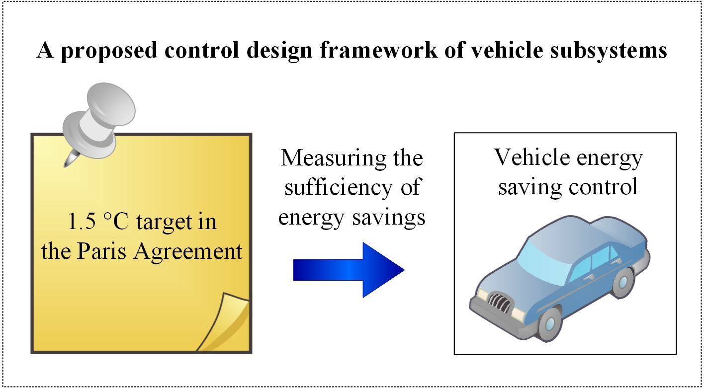
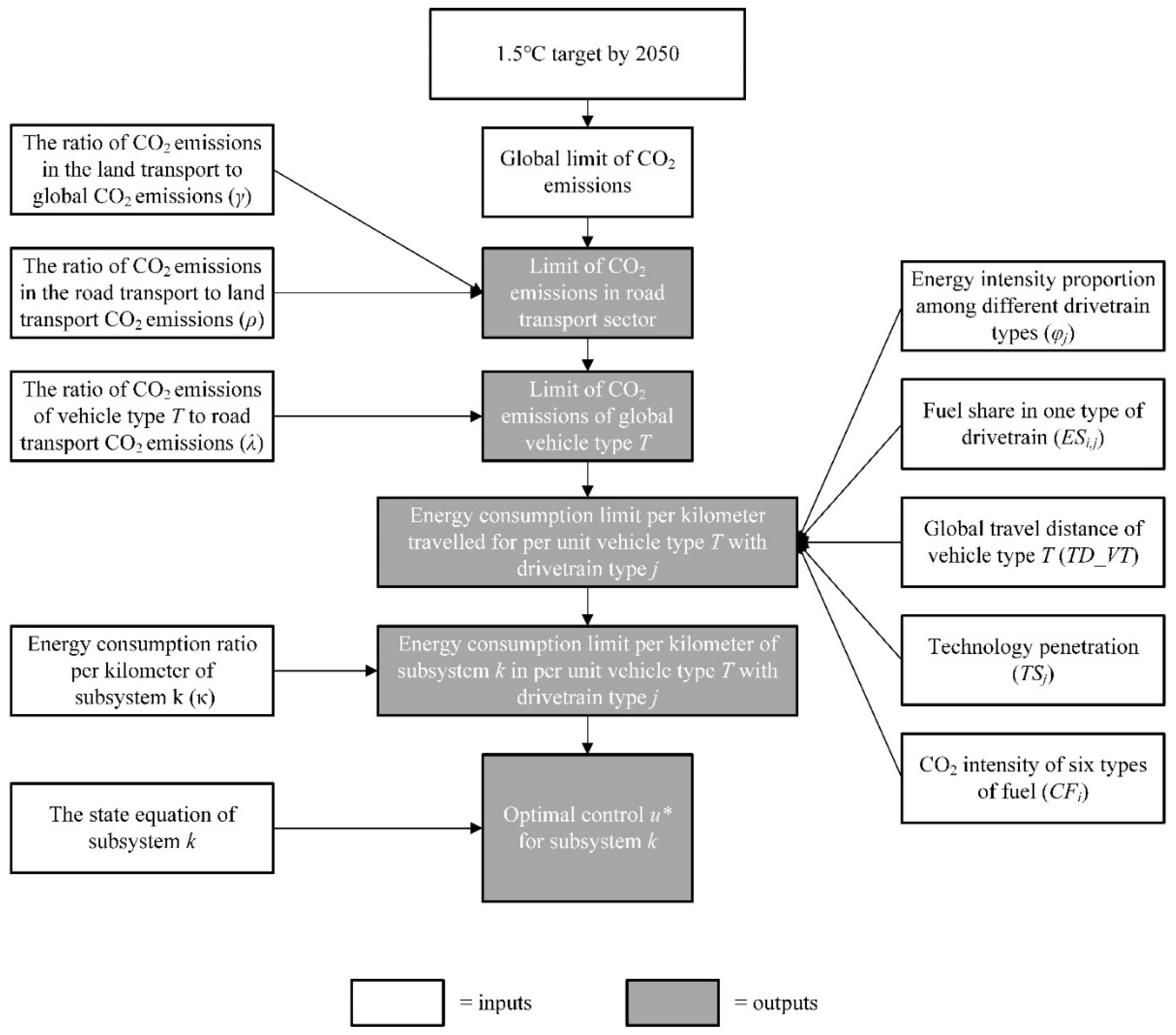
2.1. Overarching Methods

This section presents the control design framework for vehicle subsystems to meet the 1.5 °C target, consisting of five main steps as shown in Figure 1.

Step 1: Figure out the global limit of CO₂ emissions at the 1.5 °C target in 2050 $C{O}_{2}Emissions\_Globa{l}_{1.5°\mathrm{C}}$ (GtCO₂).

Step 2: Figure out the limit of CO₂ emissions in the road transport sector at the 1.5 °C target in 2050 $C{O}_{2}Emissions\_RoadTranspor{t}_{1.5°\mathrm{C}}$ (GtCO₂), as follows:

$$C{O}_{2}Emissions\_RoadTranspor{t}_{1.5°\mathrm{C}}=C{O}_{2}Emissions\_Globa{l}_{1.5°\mathrm{C}}\times \gamma \times \rho$$

(1)

where $\gamma$ is the ratio of CO₂ emissions in the land transport to global CO₂ emissions; $\rho$ is the ratio of CO₂ emissions in the road transport to land transport CO₂ emissions.

Step 3: Figure out the limit of CO₂ emissions of global vehicle type T at the 1.5 °C target in 2050 $C{O}_{2}Emissions\_V{T}_{1.5°\mathrm{C}}$ [GtCO₂] and the energy consumption limit per kilometer traveled for per unit vehicle type T with drivetrain type j $E{C}_j\_V{T}_{1.5°\mathrm{C}}$ (MJ/(vehicle km)), which are calculated by Equations (2) to (5). Referring to [16], we classify vehicles into three major types according to the drivetrain, including internal combustion engine vehicles (ICEVs), electric vehicles (EVs), and fuel cell vehicles (FCVs). ICEVs use gasoline, diesel, natural gas, or their alternative fuels to power the drivetrain. Hybrid electric vehicles (HEVs) are regarded as ICEVs characterized by higher energy efficiencies in this study. EVs are divided into two categories—BEVs and plug-in hybrid electric vehicles (PHEVs). BEVs exclusively consume electricity from a power grid. PHEVs obtain energy from both traditional fuel and grid electricity. Here PHEVs are equal to BEVs and ICEVs according to the assumed 50% share of electric drive, which means that one PHEV is equal to 0.5 ICEV and 0.5 BEV. FCVs mainly consume hydrogen to power fuel cell engines.

$$C{O}_{2}Emissions\_V{T}_{1.5°\mathrm{C}}=C{O}_{2}Emissions\_RoadTranspor{t}_{1.5°\mathrm{C}}\times \lambda$$

(2)

where $\lambda$ represents the ratio of CO₂ emissions of vehicle type T to road transport CO₂ emissions.

$$C{O}_{2}Emissions\_V{T}_{1.5°\mathrm{C}}={\displaystyle \sum _j^{}{\displaystyle \sum _i^{}TD\_VT\cdot T{S}_j\cdot E{C}_j\_V{T}_{1.5°\mathrm{C}}}}\cdot E{S}_{i,j}\cdot C{F}_i$$

(3)

$$E{C}_1\_V{T}_{1.5°\mathrm{C}}:E{C}_2\_V{T}_{1.5°\mathrm{C}}:E{C}_3\_V{T}_{1.5°\mathrm{C}}={\phi }_1:{\phi }_2:{\phi }_3$$

(4)

where ${\phi }_j$ is the proportion of the energy consumption per kilometer among different drivetrain types, and j = (1, 2, 3) represents the drivetrain of BEVs, ICEVs, and FCVs, respectively; TS_j is the share of type T vehicles with type j drivetrain out of all type T vehicles in 2050; ES_i,j is the share of energy consumption of type i fuel out of total energy consumption by type T vehicles with type j drivetrain technology in one year, and i = (1, 2, 3, 4, 5, 6) represents electricity, gasoline, diesel, bioethanol, natural gas, and hydrogen, respectively; CF_i is the CO₂ intensity of type i fuel in one year; TD_VT (vehicle km) is the global travel distance of vehicle type T in 2050, which has a relationship with the global transport demand of vehicle type T in 2050 D_T ($T\in \mathrm{Passenger}\tan \mathrm{sport}$) (passenger km (pkm)) or D_T ($T\in \mathrm{Freight}\mathrm{transport}$) (ton km (tkm)) as follows:

$$TD\_VT=\{\begin{array}{c}\begin{array}{cc}{D}_T/C_T& T\in \mathrm{Passenger}\mathrm{transport}\end{array}\\ \begin{array}{cc}{D}_T/L_T& T\in \mathrm{Freight}\mathrm{transport}\end{array}\end{array}$$

(5)

where C_T (passenger/vehicle) is the capacity per unit vehicle type T when vehicle type T belongs to passenger transport; L_T (ton/vehicle) is the load per unit vehicle type T when vehicle type T belongs to freight transport.

Step 4: Figure out the energy consumption limit per kilometer of subsystem k in per unit vehicle type T with drivetrain type j $E{C}_j\_Su{b}_{k1.5°\mathrm{C}}$ (MJ/(vehicle km)), which is considered as the limit of energy consumption used for the optimal control design for this subsystem, as follows:

$$E{C}_j\_Su{b}_{k1.5°\mathrm{C}}=E{C}_j\_V{T}_{1.5°\mathrm{C}}\times \kappa$$

(6)

where $\kappa$ is the ratio of the energy consumption per kilometer of subsystem k to the energy consumption per kilometer of per unit vehicle type T with drivetrain type j.

Finally, we conduct the optimal control design for subsystem k in vehicle type T with drivetrain type j. In our framework, the purpose of optimal control is to optimize the performance of subsystem k as much as possible, while constrained by the limit value of the energy consumption per kilometer $E{C}_j\_Su{b}_{k1.5°\mathrm{C}}$, as follows:

$$J\left(u\right)={\displaystyle {\int }_{t_0}^{T}L\left(x(t),u(t),t\right)}dt$$

(7)

subject to

$$\{\begin{array}{c}\dot{x}(t)=f\left(x(t),u(t),t\right)\\ {x(t)|}_{t=t_0}=x_0\\ u(t)\in U\\ U=g\left(E{C}_j\_Su{b}_{k1.5°\mathrm{C}}\right)\end{array}$$

(8)

where $J\left(u\right)$ is the objective function to be minimized (or maximized), x(t) is the n-dimensional state vector, $x(t)\in R^n$, u(t) is the r-dimensional control vector, $u(t)\in R^r$, $\dot{x}(t)=f\left(x(t),u(t),t\right)$ is the dynamical equality constraints initialized by ${x(t)|}_{t=t_0}=x_0$, U is used to limit the value of the control vector element $\left|u_i(t)\right|$, and in our framework U is determined by the limit value of the energy consumption per kilometer $E{C}_j\_Su{b}_{k1.5°\mathrm{C}}$.

2.2. Assumptions and Data

In our framework, it is assumed that other strategies that help to achieve the 1.5 °C target are under a business-as-usual (BAU) scenario (i.e., without additional implementation of low-carbon policies and technologies) for the purpose of obtaining a strict energy consumption limit, and consequently some parameters are also based on current or historical data such as $\rho$, ${\phi }_j$, $C{F}_i$, and $\kappa$.

2.2.1. CO₂ Emission Limits

According to [3], we can obtain the global CO₂ emissions limit in 2050 $C{O}_{2}Emissions\_Globa{l}_{1.5°\mathrm{C}}$ and the land transport emission share $\gamma$. For the ratio of CO₂ emissions in the road transport to land transport CO₂ emissions $\rho$, it is assumed to keep constant from 2016 to 2050. For the ratio of CO₂ emissions of vehicle type T to road transport CO₂ emissions $\lambda$, we used the data under a BAU scenario by 2050.

2.2.2. Travel Distance

The travel distance of vehicle type T in 2050 was obtained in terms of the transport demand of vehicle type T under a BAU scenario by 2050, distinguished from previous research [16,17] using the population of vehicle type T and the average distance traveled of vehicle type T in 2050 to estimate the travel distance. The transport demand of vehicle type T under a BAU scenario by 2050 is provided in [18].

2.2.3. Technology Penetration

For the market shares of different drivetrains, we used the data under a BAU scenario by 2050 referring to [16].

2.2.4. Energy Intensity

In this work the energy intensity is based on the New European Driving Cycle (NEDC) procedure equivalent values, which are the same as those reported in [16].

2.2.5. CO₂ Intensity

In this work the CO₂ intensity is based on the current or historical data due to the assumption that there is no additional implementation of low-carbon policies and technologies.

Estimated based on [16], the CO₂ intensities of gasoline, diesel, and compressed natural gas (CNG) are 83.16, 88.92, and 67.32 g/MJ, respectively (life cycle CO₂ emissions), and the global average CO₂ intensities of bioethanol and hydrogen are 70 g/MJ and 100 g/MJ, respectively. The global average CO₂ intensity of electricity is 573.86 g/kWh, as provided by [19].

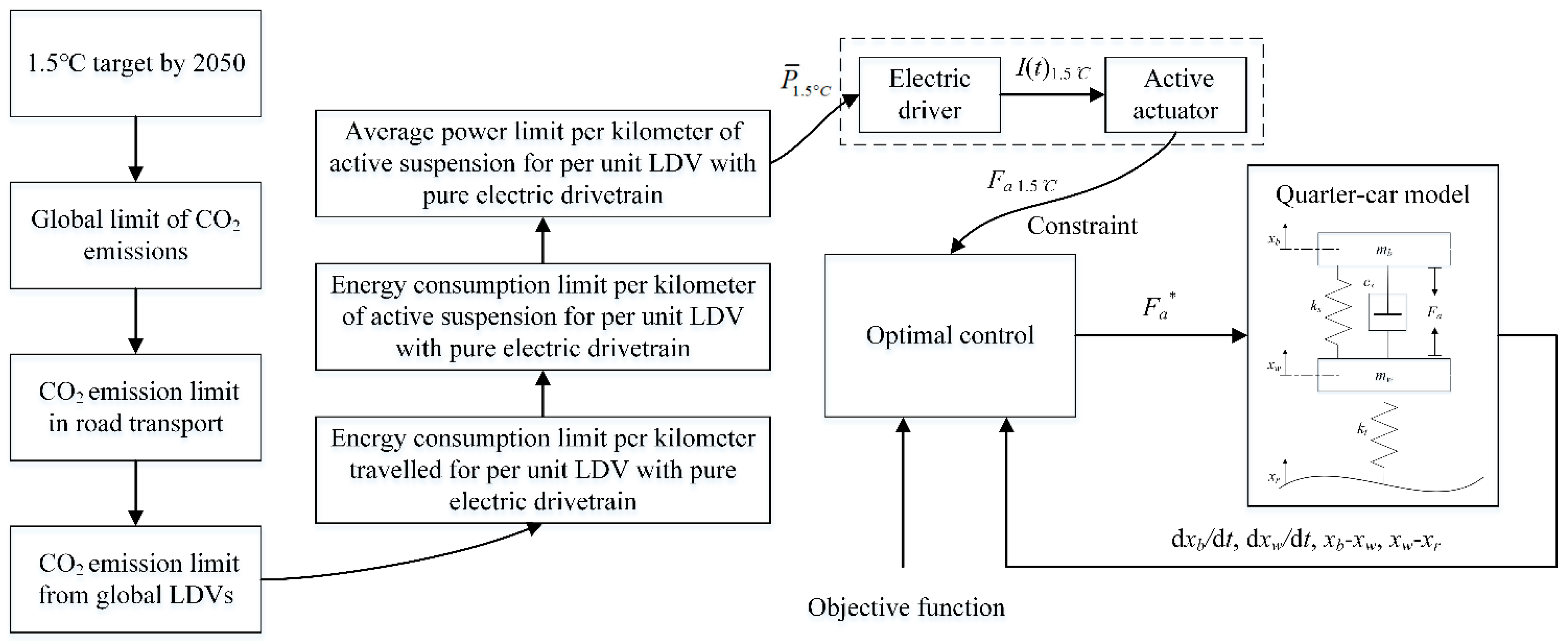
3. Case Study: Active Suspension Control for a BELDV

This section shows the specific application of the proposed control design framework for active suspension for a BELDV (or battery electric passenger car). Active suspension is a kind of electronically controllable suspension that can better suppress undesirable vibration from road roughness through controlling the active actuator force F_a.

Figure 2 shows the procedure for the application of the proposed control design framework to this case study. Firstly, based on the 1.5 °C target, the energy consumption limit of active suspension is obtained. Then, the optimal control design of active suspension is conducted with the constraint of the energy consumption limit of active suspension.

3.1. Energy Consumption Limit of Active Suspension

Based on Equations (1) to (5), the energy consumption limit of active suspension can be calculated combined with the data shown in

Table 1. Data used to obtain energy consumption limit of active suspension. BAU, business as usual; LDV, light-duty vehicle.

Variable	Value	Scenario/Year	Source/Note
CO2Emissions_Global1.5 °C (GtCO2)	10.9	1.5 °C	[3]
$\gamma$ (%)	19	1.5 °C	[3]
$\rho$ (%)	98	2016	[22]
$\lambda$ (%)	46	BAU	[18]
DLDVs (passenger km)	6.56 × 1012	BAU	[18]
CLDV (passenger/vehicle)	1		Assumption that one LDV is used by only one passenger
TS1 (%)	22.5	BAU	[16]
TS2 (%)	67.5	BAU	[16]
TS3 (%)	10	BAU	[16]
ES1,1 (%)	100	BAU	-
ES2,2 (%)	82.15	BAU	[23]
ES3,2 (%)	8.01	BAU	[23]
ES4,2 (%)	5.01	BAU	[23]
ES5,2 (%)	4.83	BAU	[23]
ES6,3 (%)	100	BAU	-
${\phi }_1:{\phi }_2:{\phi }_3$	0.54:1.5:0.74	2017	[16]
CF1 (g/kWh)	573.86	2017	[19]
CF2 (g/MJ)	83.16	2016	[16]
CF3 (g/MJ)	88.92	2016	[16]
CF4 (g/MJ)	70	2000	[16]
CF5 (g/MJ)	67.32	2016	[16]
CF6 (g/MJ)	100	2020	[16]
$\kappa$ (%)	50	2010, 2016	[20,21]

. The detailed steps are presented as follows:

3.1.1. Step1: CO₂Emissions_Global_{1.5 °C}

Adopted from [3], the global limit of CO₂ emissions at the 1.5 °C target by 2050 CO₂ Emissions_Global_{1.5 °C} is 10.9 GtCO₂.

3.1.2. Step2: CO₂Emissions_RoadTransport_{1.5 °C}

Using Equation (1), the limit of CO₂ emissions in the road transport sector under the 1.5 °C target in 2050 $C{O}_{2}Emissions\_RoadTranspor{t}_{1.5°\mathrm{C}}$ can be calculated as 2.0588 GtCO₂.

3.1.3. Step3: EC₁_VLDV_{1.5 °C}

Using Equation (2), the limit of CO₂ emissions from global light-duty vehicles (LDVs) (or passenger cars) under the 1.5 °C target in 2050 $C{O}_{2}Emissions\_VLDV{s}_{1.5°\mathrm{C}}$ can be calculated as 0.9474 GtCO₂.

It should be noted that C_LDV (passenger/vehicle) is assumed to be 1 (i.e., one LDV is used by only one passenger) in this study in order to obtain a strict energy consumption limit. Using Equations (3) to (5), the energy consumption per kilometer traveled for per unit LDV with a pure electric drivetrain $E{C}_1\_VLD{V}_{1.5°\mathrm{C}}$ can be calculated as 0.709 MJ/(vehicle km).

3.1.4. Step4: EC₁_Sub_{active-sus1.5 °C}

Based on [20,21], using Equation (6), the obtained energy consumption limit of active suspension for per unit LDV with pure electric drivetrain $E{C}_1\_Su{b}_{active-sus1.5°\mathrm{C}}$ is 0.355 MJ/(vehicle km), which provides the key constraint for the optimal control design under the 1.5 °C target. Note that $\kappa$ is obtained by the current energy consumption per kilometer of active suspension divided by the current energy consumption per kilometer of per unit BELDV. Referring to [20], the current energy consumption per kilometer of active suspension (148.9 Wh/km) is calculated based on the NEDC procedure. The current energy consumption per kilometer of per unit BELDV (297.4 Wh/km) is based on the NEDC procedure value adopted from [21].

3.2. Control Design

Under the constraint of the energy consumption limit of active suspension, the optimal control design of active suspension is conducted. The vertical quarter-car model is used in the optimal control design for improving the performance including the ride comfort, road holding ability, and suspension physical constraint satisfaction. The performance indexes corresponding to ride comfort, road holding ability, and suspension physical constraint satisfaction are body vertical acceleration, tire deflection, and suspension deflection, respectively.

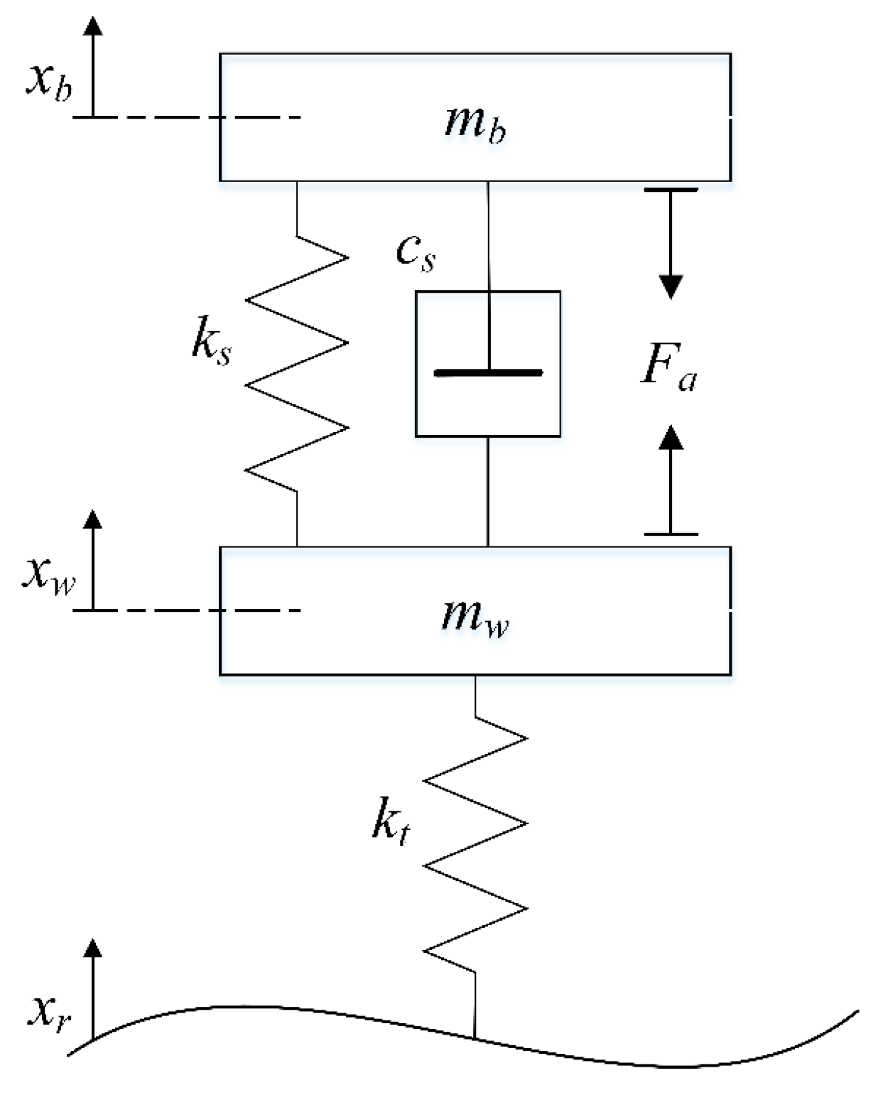
3.2.1. Vertical Quarter-Car Model

The linear vertical quarter-car model is a simplified suspension model based on the following assumptions: (a) the suspension deflection is within the limit stroke range and the suspension will not be penetrated during operation; (b) car seat dynamics are not considered, and the tire stiffness is constant; (c) the car seat is rigidly interconnected with the body, the axle and the tire are rigidly connected to each other; and (d) road excitation is consistent for the left and right wheels, and the suspension mass distribution factor is assumed to be 1 [24].

The vertical quarter-car model is depicted by Figure 3. It contains four state variables: the sprung mass velocity $x_1={\dot{x}}_b$, the unsprung mass velocity $x_2={\dot{x}}_w$, the sprung mass displacement $x_3=x_b-x_w$, and the unsprung mass displacement $x_4=x_w-x_r$. The model parameters are based on [25]: m_b = 240 kg, m_w = 36 kg, c_s = 980 N s/m, k_s = 16,000 N/m, and k_t = 160,000 N/m.

The system is described by the following state equations:

$$\{\begin{array}{c}{m}_b{\dot{x}}_1=-k_s{x}_3-c_s(x_1-x_2)-F_a\\ m_w{\dot{x}}_2=k_s{x}_3+c_s(x_1-x_2)-k_t{x}_4+F_a\\ {\dot{x}}_3=x_1-x_2\\ {\dot{x}}_4=x_2-{\dot{x}}_r\end{array}$$

(9)

where x_r is the road vertical displacement, ${\dot{x}}_r$ is the road vertical velocity, and F_a is the active actuator force (i.e., the control input).

In active suspension, the energy is consumed to generate the active actuator force F_a to protect the body from vibration due to road roughness. Thus, the energy consumption of active suspension can be calculated by Equation (10).

$$\{\begin{array}{c}P(t)=F_a({\dot{x}}_b-{\dot{x}}_w)\\ E{C}_{active-sus}={\displaystyle {\int }_0^{{\overline{t}}_{1\mathrm{k}\mathrm{m}}}P(t)dt}\end{array}$$

(10)

where P(t) is the power consumed by active suspension. $E{C}_{active-sus}$ is the energy consumed by active suspension per kilometer. ${\overline{t}}_{1\mathrm{k}\mathrm{m}}$ = 107 s is the average period taken by a BELDV traveling one kilometer under an NEDC.

Under the 1.5 °C target, the energy consumption per kilometer of active suspension is constrained by the limit $E{C}_1\_Su{b}_{active-sus1.5°\mathrm{C}}$, as shown in Equation (11).

$$E{C}_{active-sus}\le E{C}_1\_Su{b}_{active-sus1.5°\mathrm{C}}$$

(11)

The limit $E{C}_1\_Su{b}_{active-sus1.5°\mathrm{C}}$ can be represented by Equation (12).

$$E{C}_1\_Su{b}_{active-sus1.5°\mathrm{C}}=4\cdot {\overline{P}}_{1.5°\mathrm{C}}\cdot {\overline{t}}_{1\mathrm{k}\mathrm{m}}$$

(12)

where ${\overline{P}}_{1.5°\mathrm{C}}$ = 828.3 W is the average power limit of active suspension in the quarter-car under the 1.5 °C target.

Therefore, Equation (12) can be expressed as Equation (13).

$${\displaystyle {\int }_0^{{\overline{t}}_{1km}}P(t)dt}\le {\overline{P}}_{1.5°\mathrm{C}}\cdot {\overline{t}}_{1\mathrm{k}\mathrm{m}}.$$

(13)

In order to meet Equation (13), (14) is obtained.

$$P(t)\le {\overline{P}}_{1.5°\mathrm{C}}.$$

(14)

Considering Equations (10) and (14) together, the constraint on actuator force is expressed as:

$$-\left|F_a\left({\overline{P}}_{1.5°\mathrm{C}}\right)\right|\le F_a\left(P(t),t\right)\le \left|F_a\left({\overline{P}}_{1.5°\mathrm{C}}\right)\right|.$$

(15)

3.2.2. Design of Optimal Control

For the optimal control issue where the control variable u is constrained, Pontryagin’s Minimum Principle is utilized to find the optimal control input u^*.

The objective function is written as Equation (16).

$$J={\beta }_1{\displaystyle {\int }_0^{t_f}{\dot{x}}^2{}_1}dt+{\beta }_2{\displaystyle {\int }_0^{t_f}{(x_4-x_r)}^2}dt+{\beta }_3{\displaystyle {\int }_0^{t_f}{(x_3-x_4)}^2}dt+{\beta }_4{\displaystyle {\int }_0^{t_f}{u}^2}dt$$

(16)

where ${\dot{x}}_1$ is the body vertical acceleration, $x_4-x_r$ is the tire deflection, and $x_3-x_4$ is the suspension deflection. ${\beta }_1$, ${\beta }_2$, and ${\beta }_3$ are the weighting factors serving as tuning parameters that affect the compromise among ride comfort performance, road holding ability, and suspension physical constraint satisfaction. Small body vertical acceleration means good ride comfort. Small tire deflection and suspension deflection indicate good road holding performance. Their default values ${\beta }_1=1$, ${\beta }_2=1100$, and ${\beta }_3=100$ are adopted from [25]. The weighting factor of the control input ${\beta }_4=0.0001$ is based on [25].

In this case study, F_a is the control input and ${\dot{x}}_r$ is considered as the external disturbance. The linear vertical quarter-car model, described as Equation (9), is extended for the control design as:

$$\{\begin{array}{c}\begin{array}{c}\dot{x}=Ax+Bu+G{\dot{x}}_r\\ y=Cx+Du\end{array}\\ {x|}_0=0\end{array}$$

(17)

where

$$x=\left[\begin{array}{c}{x}_1\\ x_2\\ x_3\\ x_4\end{array}\right]A=\left[\begin{array}{cccc}-c_s/m_b& c_s/m_b& -k_s/m_b& 0\\ c_s/m_w& -c_s/m_w& k_s/m_w& -k_t/m_w\\ 1& -1& 0& 0\\ 0& 1& 0& 0\end{array}\right]B=\left[\begin{array}{c}-1/m_b\\ 1/m_w\\ 0\\ 0\end{array}\right]$$

$$C=\left[\begin{array}{cccc}-c_s/m_b& c_s/m_b& -k_s/m_b& 0\\ 0& 0& 1& 0\\ 0& 0& 0& 1\end{array}\right]D=\left[\begin{array}{c}-1/m_b\\ 0\\ 0\end{array}\right]u=F_{a}G=\left[\begin{array}{c}0\\ 0\\ 0\\ -1\end{array}\right]$$

The objective function is re-derived as Equation (18).

$$J=\frac{1}{2}{\displaystyle {\int }_0^{t_f}(x^{\mathrm{T}}Qx+u^{\mathrm{T}}Ru+x^{\mathrm{T}}Nu+u^{\mathrm{T}}{N}^{\mathrm{T}}x)dt}$$

(18)

where

$$Q=C^{\mathrm{T}}{Q}_{\mathrm{P}}C·R=R_1+R_2·N=C^{\mathrm{T}}{Q}_{\mathrm{P}}D·Q_{\mathrm{P}}=diag(\begin{array}{ccc}2{\beta }_1& 2{\beta }_3& 2{\beta }_2\end{array})·R_1=[2{\beta }_4]·R_2=D^{\mathrm{T}}{Q}_{\mathrm{P}}D.$$

The Hamiltonian function is given by Equation (19).

$$H=\frac{1}{2}{x}^{\mathrm{T}}Qx+\frac{1}{2}{u}^{\mathrm{T}}Ru+\frac{1}{2}{x}^{\mathrm{T}}Nu+\frac{1}{2}{u}^{\mathrm{T}}{N}^{\mathrm{T}}x+{\lambda }^{\mathrm{T}}(Ax+Bu)$$

(19)

where $\lambda ={\left[\begin{array}{cccc}{\lambda }_1& {\lambda }_2& {\lambda }_3& {\lambda }_4\end{array}\right]}^{\mathrm{T}}$ are the Lagrange multipliers, which evolve according to the co-state dynamics governed by Equation (20).

$$\{\begin{array}{c}\dot{\lambda }=-\frac{\partial H}{\partial x}\begin{array}{cc}& \lambda (t_f)=0\end{array}\\ \lambda =Sx\end{array}.$$

(20)

It can be seen from Equation (19) that H is the quadratic parabolic function of u, and there exists u ($-\left|F_a\left({\overline{P}}_{1.5°\mathrm{C}}\right)\right|\le u\le \left|F_a\left({\overline{P}}_{1.5°\mathrm{C}}\right)\right|$ according to Equation (15), making H have a minimum. Firstly, the control input u_min that minimizes H can be obtained by Equation (21), and the details about Equations (20) to (22) are presented in Appendix A.

$$\frac{\partial H}{\partial u}=0,$$

(21)

$$u_{\min }=-R^{-1}(B^{\mathrm{T}}\lambda +N^{\mathrm{T}}x).$$

(22)

Finally, according to Pontryagin’s Minimum Principle, the optimal actuator force is expressed as Equation (23).

$$F_a^{*}=u^{*}=\{\begin{array}{cc}-\left|F_a\left({\overline{P}}_{1.5°\mathrm{C}}\right)\right|& u_{\min }<-\left|F_a\left({\overline{P}}_{1.5°\mathrm{C}}\right)\right|\\ u_{\min }& -\left|F_a\left({\overline{P}}_{1.5°\mathrm{C}}\right)\right|\le u_{\min }\le \left|F_a\left({\overline{P}}_{1.5°\mathrm{C}}\right)\right|\\ \left|F_a\left({\overline{P}}_{1.5°\mathrm{C}}\right)\right|& u_{\min }>\left|F_a\left({\overline{P}}_{1.5°\mathrm{C}}\right)\right|\end{array}.$$

(23)

3.3. Evaluation

This section utilizes the widely used LQR method [8] as a basis for comparison to evaluate the proposed control design framework. Specifically, the performance and energy consumption of the proposed framework are compared with those of the LQR method.

3.3.1. A Widely Used LQR Optimal Control for Comparison

The LQR method is utilized to design the optimal control. By solving the Riccati Equation (24), matrix $\overline{P}$ can be obtained. Then the optimal control is obtained as Equation (25).

$$-\overline{P}A-A^{\mathrm{T}}\overline{P}+(\overline{P}B+N)R^{-1}(B^T\overline{P}+N^T)-Q=0,$$

(24)

$$u^{*}=-R^{-1}(B^{\mathrm{T}}\overline{P}+N^{\mathrm{T}})x.$$

(25)

3.3.2. Road Disturbance Model

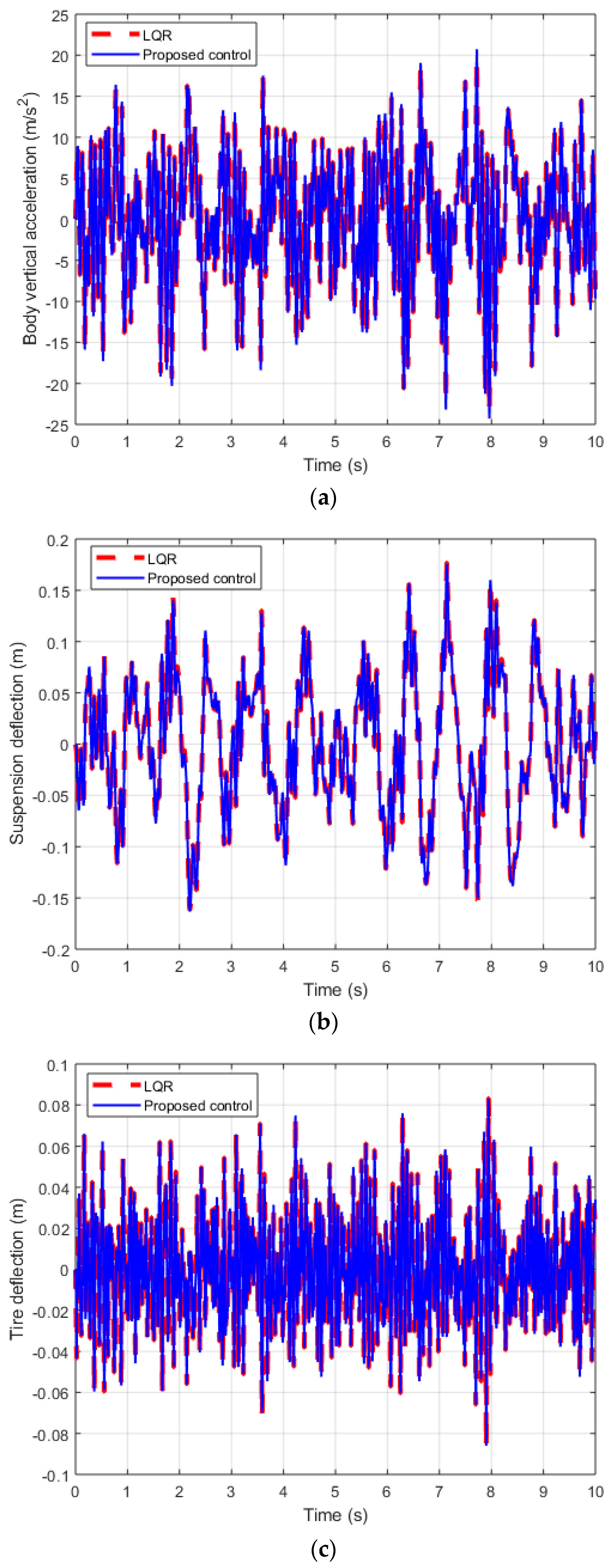
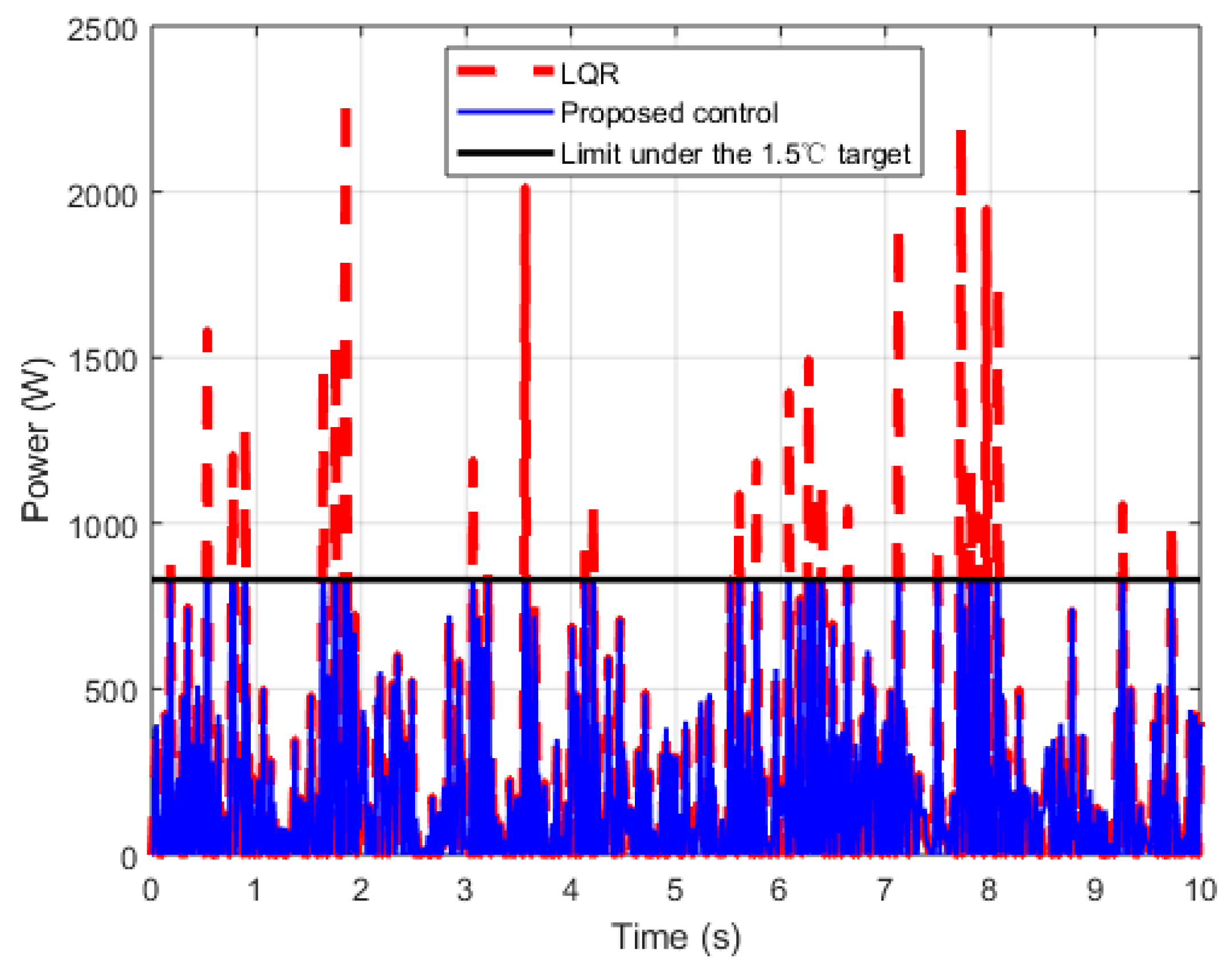
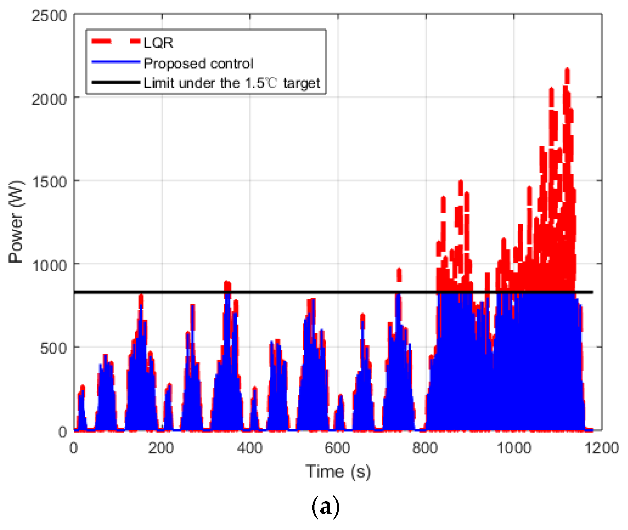
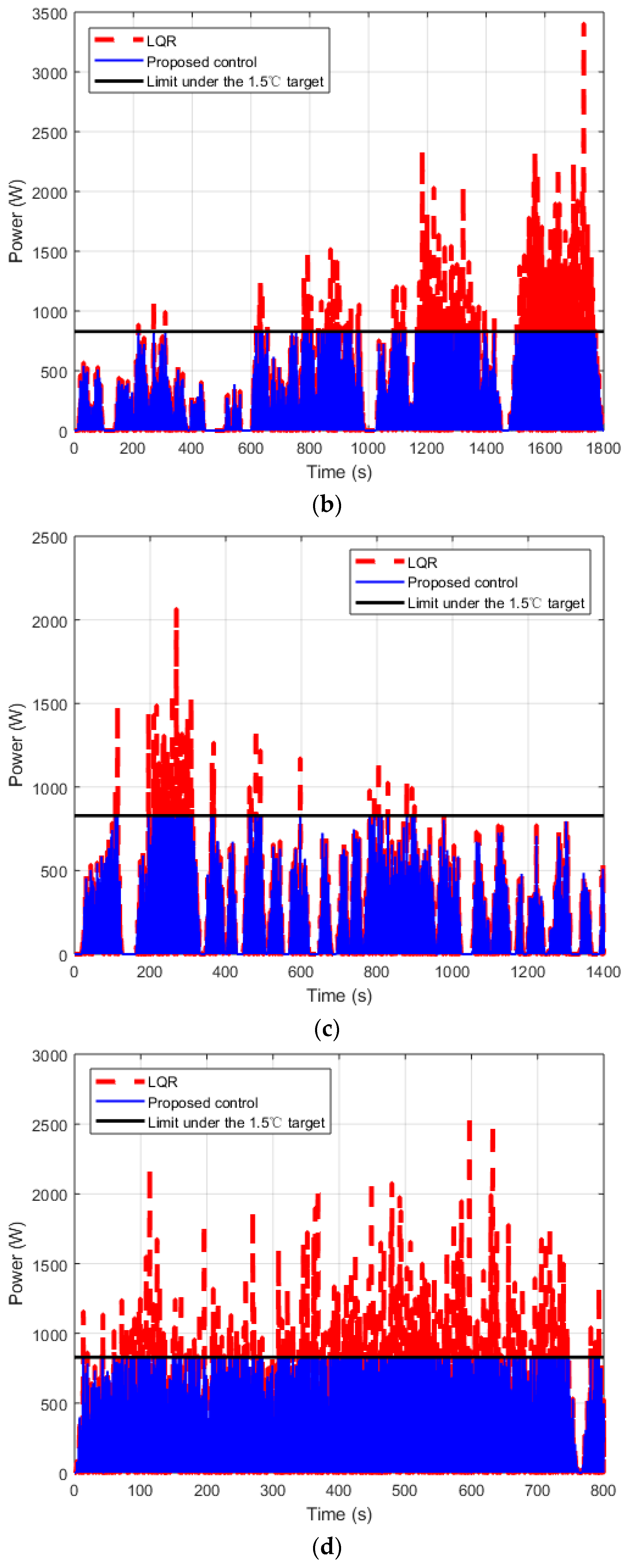
The evaluation is conducted under the following road disturbance [26]:

$${\dot{x}}_r(t)=0.111\left[40w_0(t)\sqrt{G_q(n_0)v(t)}-v(t)x_r(t)\right]$$

(26)

where ${\dot{x}}_r$ is the road vertical velocity, x_r is the road vertical displacement, w₀(t) is the Gaussian white noise with zero mean value, G_q (n₀) is the road roughness coefficient, n₀ represents the spatial frequency value, and v(t) represents the vehicle speed in m/s.

According to [27], road profiles are classified into levels A–H to describe various road roughness levels. The classification criteria for road levels A–H are shown in

Table 2. Classification standard of road levels A–H.

Level	Degree of Roughness Gq(n0) (10−6 m2/m−1) n0 = 0.1 m−1
	Lower Limit	Geometric Mean	Upper Limit
A	8	16	32
B	32	64	128
C	128	256	512
D	512	1024	2048
E	2048	4096	8192
F	8192	16,384	32,768
G	32,768	65,536	131,072
H	131,072	262,144	524,288

.

3.3.3. Results

The evaluation results are reflected by the root mean square (RMS) values of performance indexes under road disturbance, including body vertical acceleration, suspension deflection, and tire deflection. A small body vertical acceleration means good ride comfort. A small tire deflection and suspension deflection indicate good road holding performance.

Firstly, the road level F and vehicle speed 10 m/s were chosen to generate the road disturbance, because the road level F is generally the upper limit of road roughness for LDVs and 10 m/s is proper for a vehicle driving on the road level F. As shown in Figure 4, under this road disturbance, the proposed control is comparable to the LQR from the perspective of the performance index. The detailed RMS values of performance indexes are presented in

Table 3. Performance index root mean square (RMS) value comparison between the proposed control and the linear quadratic regulator (LQR).

Performance Index	LQR	Proposed Control
Body vertical acceleration (m/s2)	7.29	7.32
Suspension deflection (m)	0.0644	0.0645
Tire deflection (m)	0.0247	0.0247

. However, from the perspective of energy consumption, Figure 5 shows that the power consumption of the LQR exceeds the limit and does not meet the 1.5 °C target, while the proposed control is within the power limit under the 1.5 °C target.

Furthermore, the road level E and different driving cycles, including the NEDC, Worldwide Harmonized Light-Duty Driving Test Cycle (WLTC), Urban Dynamometer Driving Schedule (UDDS), and Highway Fuel Economy Test Cycle (HWFET), were combined to generate the road disturbance to evaluate the proposed control design framework under different combination scenarios, as presented in

Table 4. Different combination scenarios of road levels and driving cycle inputs.

Scenario	Road Level	Driving Cycle
1	E	New European Driving Cycle (NEDC)
2	E	Worldwide Harmonized Light-Duty Driving Test Cycle (WLTC)
3	E	Urban Dynamometer Driving Schedule (UDDS)
4	E	Highway Fuel Economy Test Cycle (HWFET)

.

Figure 6 illustrates the performance index comparison between different scenarios. For the RMS value of body vertical acceleration, the proposed control is slightly larger than the LQR. For the RMS values of suspension deflection and tire deflection, the proposed control is smaller than the LQR. In summary, the proposed control is comparable to the LQR in terms of performance.

As for energy consumption, as shown in Figure 7, the proposed control is within the 1.5 °C target power limit in these four scenarios, while the LQR exceeds the limit.

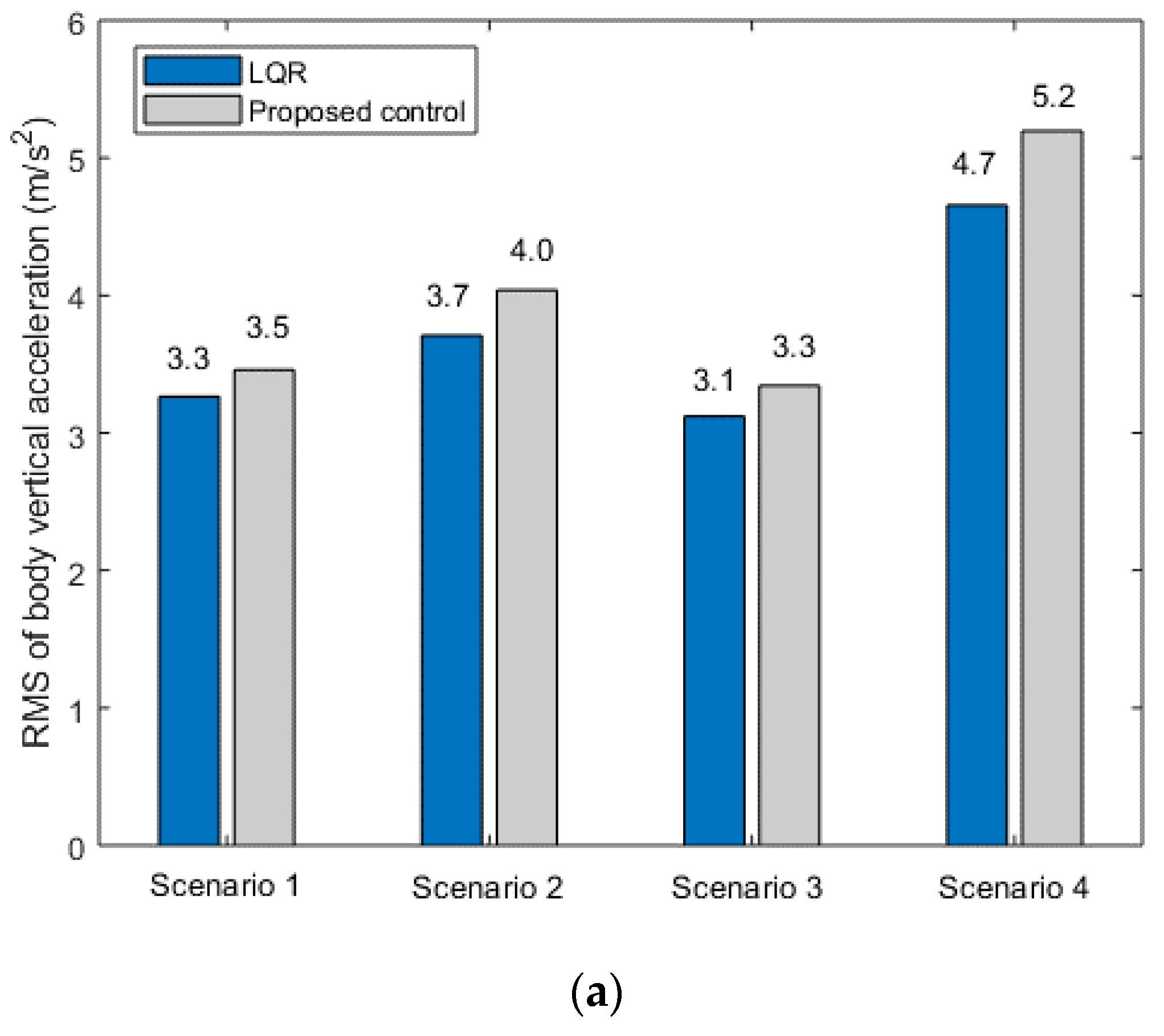
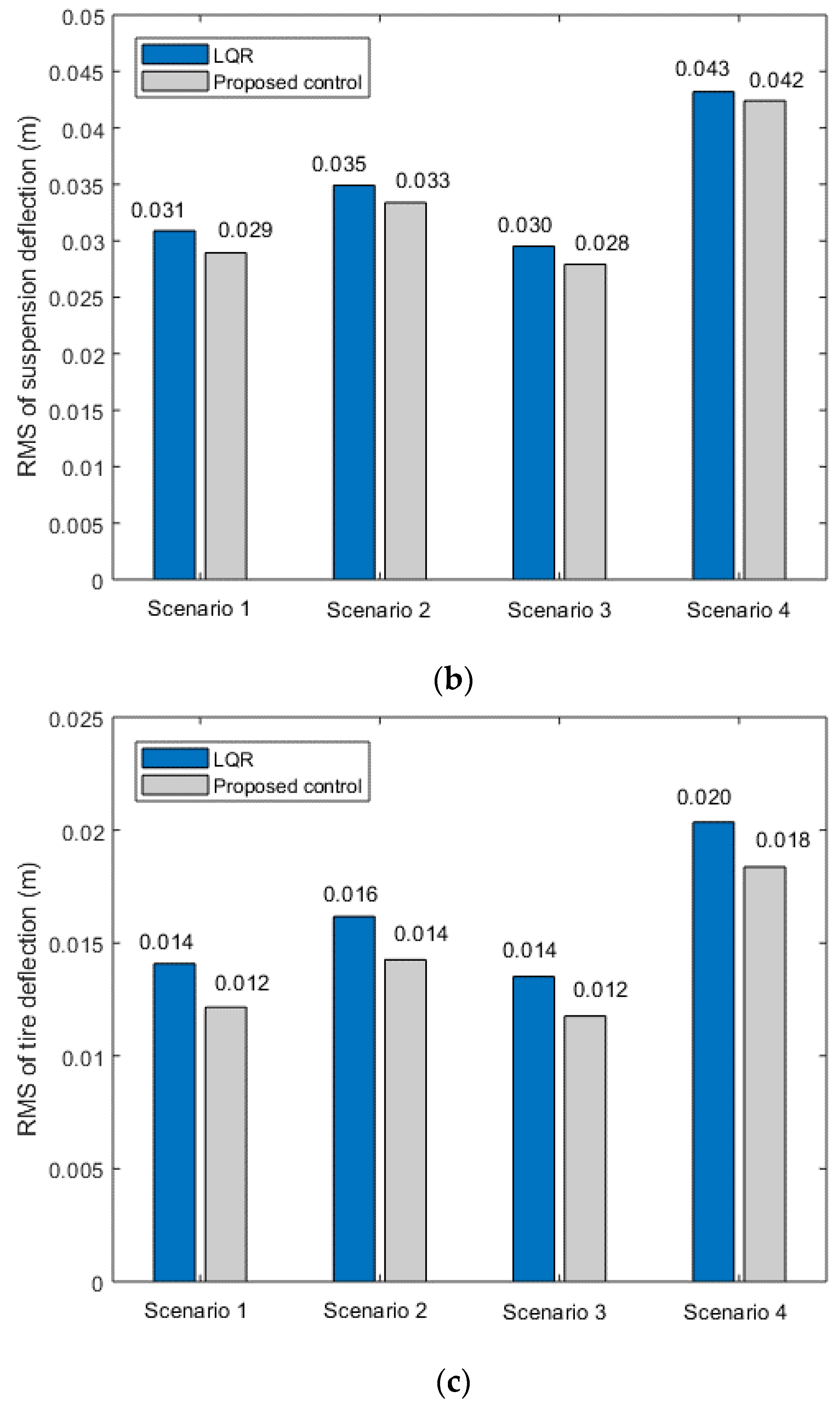
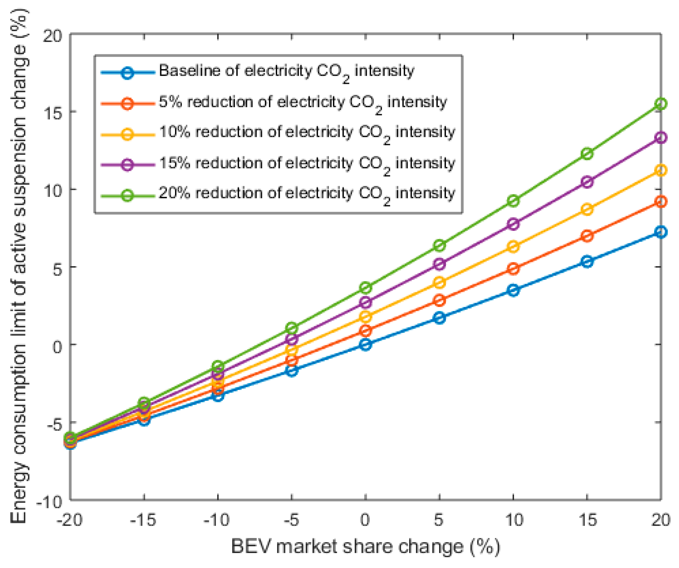
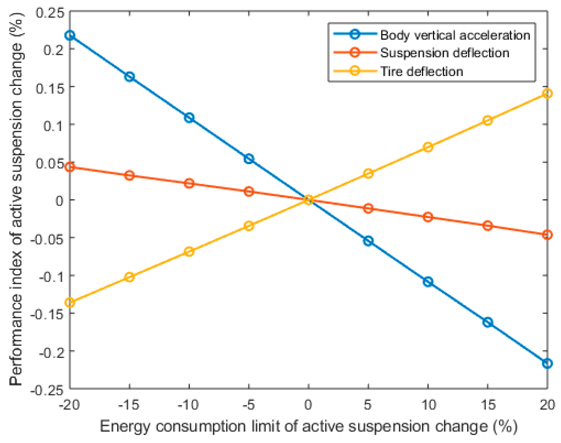
3.4. Sensitivity Analysis

Additional low-carbon policies and technologies will be implemented in the future. Technology penetration and CO₂ intensity are two main change factors. This case study is concerned with BELDVs. Therefore, the impacts of BEV market share and electricity CO₂ intensity on the energy consumption limit of active suspension under the 1.5 °C target are analyzed. Furthermore, the impacts of the 1.5 °C target active suspension energy consumption limit on the active suspension performance index are investigated. All the baselines concerning BEV market share, electricity CO₂ intensity, energy consumption limit of active suspension under the 1.5 °C target, and the active suspension performance index are the values from the above case study.

Figure 8 describes the impacts of BEV market share and electricity CO₂ intensity on the energy consumption limit of active suspension under the 1.5 °C target. To obtain Figure 8, firstly, with electricity CO₂ intensity maintained at baseline and BEV market share changing from −20 to 20%, the energy consumption limit of active suspension change relative to baseline can be determined based on the calculation in Section 3.1. This calculation gives the blue line in Figure 8. Then, with electricity CO₂ intensity decreasing 5% and BEV market share changing from −20 to 20%, the energy consumption limit of active suspension change relative to baseline can be calculated, giving the red line in Figure 8. The other three lines in Figure 8 were obtained through similar processes.

As shown in Figure 8, with the increase of BEV market share, the energy consumption limit of active suspension under the 1.5 °C target decreases. The rise of BEV market share change has a greater impact on the energy consumption limit of active suspension under the 1.5 °C target than the decline of this variable. In addition, the reduction of electricity CO₂ intensity raises the energy consumption limit of active suspension under the 1.5 °C target.

Figure 9 describes the effect of the 1.5 °C target active suspension energy consumption limit on the active suspension performance indexes including body vertical acceleration, suspension deflection, and tire deflection. With the consumption limit of active suspension changing from −20 to 20%, body vertical acceleration can be obtained, which is represented by the blue line in Figure 9. Similarly, the other two lines in Figure 9 were obtained.

As shown in Figure 9, with the rise of the 1.5 °C target active suspension energy consumption limit, body vertical acceleration and suspension deflection decrease while tire deflection increases. By contrast, body acceleration and tire deflection exhibit greater changes than suspension deflection. Still, all in all, the active suspension performance index is not sensitive to the 1.5 °C target active suspension energy consumption limit. That implies that the active suspension performance is hardly weakened, despite the constraint of the 1.5 °C target active suspension energy consumption limit.

Combining Figure 8 and Figure 9, it can be concluded that the active suspension performance index is not sensitive to BEV market share and electricity CO₂ intensity. This implies that the control effect of the proposed framework is hardly changed by BEV market share and electricity CO₂ intensity.

4. Discussion and Conclusions

Current studies have achieved energy savings of vehicle subsystems through various control strategies, but they do not measure whether these energy savings are sufficient. This work proposed a control design framework that uses the Paris Agreement as a benchmark to measure the adequacy of energy savings of vehicle subsystems. In detail, in this framework, the control is constrained by the necessity of meeting the 1.5 °C target in the Paris Climate Agreement.

First of all, the overarching methods of this control design framework were introduced, which involves two points. One is the conversion of the 1.5 °C target into a constraint on the energy consumption of a vehicle subsystem. The other is the optimal control design of the vehicle subsystem under this constraint.

Then we conducted a case study concerning the control design of active suspension in a BELDV to describe the specific application of the proposed control design framework. Based on the 1.5 °C target, the energy consumption limit (0.355 MJ/(vehicle km)) of active suspension was obtained. Under the constraint of the energy consumption limit of active suspension, the optimal control design of active suspension was conducted.

To evaluate the proposed control design framework, the widely used LQR method was utilized as a basis for comparison under different combination scenarios of road levels and driving cycle inputs. From the perspective of performance, the proposed control is comparable to LQR. From the perspective of energy consumption, the power consumption of LQR exceeds the limit and does not meet the 1.5 °C target, while the proposed control is within the power limit under the 1.5 °C target. Moreover, the impacts of BEV market share and electricity CO₂ intensity on the energy consumption limit of active suspension under the 1.5 °C target and active suspension performance index were investigated. We found that the control effect of the proposed framework is hardly changed by BEV market share and electricity CO₂ intensity.

These findings imply that the proposed control design framework can both ensure the performance and help to meet the 1.5 °C target in the Paris Climate Agreement. This work offers a method for measuring the adequacy of energy-saving control of vehicle subsystems. In addition, for the applicability of the proposed control design framework in industries, it might provide a method for the automotive industry to take action to contribute to the Paris Agreement.

For future research, since the embedded systems can conflict each other, it is suggested that more than one system be considered and the control distribution be optimized.

References

1. PricewaterhouseCoopers LLP. The World in 2050: Can Rapid Global Growth Be Reconciled with Moving to a Low Carbon Economy. 2008. Available online: https://www.pwc.com/gx/en/psrc/pdf/world_in_2050_carbon_emissions_psrc.pdf (accessed on 29 May 2019).
2. United Nations Framework Convention on Climate Change (UNFCCC). Paris Agreement–Pre 2020 Action. 2016. Available online: www.ec.europa.eu/clima/policies/international/negotiations/paris/index_en.htm (accessed on 10 June 2019).
3. Paris Process on Mobility and Climate (PPMC). Implications of 2DS and 1.5DS for Land Transport Carbon Emissions in 2050. 2016. Available online: http://www.ppmc-transport.org/implications-of-2ds-and-1-5ds-for-land-transport-carbon-emissions-in-2050/ (accessed on 31 May 2019).
4. World Energy Council (WEC). Global Transport Scenarios 2050. 2012. Available online: https://www.worldenergy.org/wp-content/uploads/2012/09/wec_transport_scenarios_2050.pdf (accessed on 31 May 2019).
5. Geng, G.; Shen, Q.; Jiang, H. ANFTS Mode Control for an Electronically Controlled Hydraulic Power Steering System on a Permanent Magnet Slip Clutch. Energies 2019, 12, 1739. [Google Scholar] [CrossRef]
6. Hanifah, R.A.; Toha, S.F.; Hassan, M.K.; Ahmad, S. Power reduction optimization with swarm based technique in electric power assist steering system. Energy 2016, 102, 444–452. [Google Scholar] [CrossRef]
7. Edrén, J.; Jonasson, M.; Jerrelind, J.; Trigell, A.S.; Drugge, L. Energy efficient cornering using over-actuation. Mechatronics 2019, 59, 69–81. [Google Scholar] [CrossRef] [Green Version]
8. Han, Z.; Xu, N.; Chen, H.; Huang, Y.; Zhao, B. Energy-efficient control of electric vehicles based on linear quadratic regulator and phase plane analysis. Appl. Energy 2018, 213, 639–657. [Google Scholar] [CrossRef]
9. Khayyam, H. Adaptive intelligent control of vehicle air conditioning system. Appl. Therm. Eng. 2013, 51, 1154–1161. [Google Scholar] [CrossRef]
10. Lim, T.H.; Shin, Y.; Kim, S.; Kwon, C. Predictive control of car refrigeration cycle with an electric compressor. Appl. Therm. Eng. 2017, 127, 1223–1232. [Google Scholar] [CrossRef]
11. Huang, Y.; Khajepour, A.; Ding, H.; Bagheri, F.; Bahrami, M. An energy-saving set-point optimizer with a sliding mode controller for automotive air-conditioning/refrigeration systems. Appl. Energy 2017, 188, 576–585. [Google Scholar] [CrossRef]
12. Li, L.; Li, X.; Wang, X.; Song, J.; He, K.; Li, C. Analysis of downshift’s improvement to energy efficiency of an electric vehicle during regenerative braking. Appl. Energy 2016, 176, 125–137. [Google Scholar] [CrossRef]
13. Ruan, J.; Walker, P.D.; Watterson, P.A.; Zhang, N. The dynamic performance and economic benefit of a blended braking system in a multi-speed battery electric vehicle. Appl. Energy 2016, 183, 1240–1258. [Google Scholar] [CrossRef]
14. Casavola, A.; Iorio, F.D.; Tedesco, F. A multiobjective H∞ control strategy for energy harvesting in regenerative vehicle suspension systems. Int. J. Control 2018, 91, 741–754. [Google Scholar] [CrossRef]
15. Hsieh, C.; Huang, B.; Golnaraghi, F.; Moallem, M. Regenerative Skyhook Control for an Electromechanical Suspension System Using a Switch-Mode Rectifier. IEEE Trans. Veh. Technol. 2016, 65, 9642–9650. [Google Scholar] [CrossRef]
16. Hao, H.; Geng, Y.; Sarkis, J. Carbon footprint of global passenger cars: Scenarios through 2050. Energy 2016, 101, 121–131. [Google Scholar] [CrossRef]
17. Gambhir, A.; Tse, L.; Tong, D.; Martinez-Botas, R. Reducing China’s road transport sector CO2 emissions to 2050: Technologies, costs and decomposition analysis. Appl. Energy 2015, 157, 905–917. [Google Scholar] [CrossRef]
18. Dhar, S.; Pathak, M.; Shukla, P.R. Transformation of India’s transport sector under global warming of 2 °C and 1.5 °C scenario. J. Clean. Prod. 2018, 172, 417–427. [Google Scholar] [CrossRef]
19. Mora, C.; Rollins, R.; Taladay, K.; Kantar, M.B.; Chock, M.K.; Shimada, M.; Franklin, E.C. Bitcoin emissions alone could push global warming above 2 °C. Nat. Clim. Change 2018, 8, 931–933. [Google Scholar] [CrossRef]
20. Savaresi, S.M.; Poussot-Vassal, C.; Spelta, C.; Sename, O.; Dugard, L. Semi-Active Suspension Control Design for Vehicles; Butterworth-Heinemann: Boston, MA, USA, 2010; pp. 23–25. [Google Scholar]
21. Fiori, C.; Ahn, K.; Rakha, H.A. Power-based electric vehicle energy consumption model: Model development and validation. Appl. Energy 2016, 168, 257–268. [Google Scholar] [CrossRef]
22. United Nations Framework Convention on Climate Change (UNFCC). Greenhouse Gas Inventory Data–Detailed Data by Party. 2016. Available online: https://di.unfccc.int/detailed_data_by_party (accessed on 10 June 2019).
23. Takeshita, T. Global Scenarios of Air Pollutant Emissions from Road Transport through to 2050. Int. J. Environ. Res. Public Health 2011, 8, 3032–3062. [Google Scholar] [CrossRef] [PubMed]
24. Yu, Z.; Xia, Q. Automobile Theory, 5th ed.; China Machine Press: Beijing, China, 2009; pp. 212–213. [Google Scholar]
25. Čorić, M.; Deur, J.; Xu, L.; Tseng, H.E.; Hrovat, D. Optimisation of active suspension control inputs for improved vehicle ride performance. Veh. Syst. Dyn. 2016, 54, 1004–1030. [Google Scholar] [CrossRef]
26. Wu, Z.; Chen, S.; Yang, L.; Zhang, B. Model of road roughness in time domain based on rational function. Trans. Beijing Inst. Technol. 2009, 29, 795–798. [Google Scholar]
27. GB/T 7031-2005/ISO 8086. Mechanical Vibration-Road Surface Profiles—Reporting of Measured Data. Available online: https://www.iso.org/obp/ui/#iso:std:iso:8608:ed-2:v1:en (accessed on 2 August 2019).
Figure 1. Framework of optimal control design for meeting the 1.5 °C target.
Energies 12 03170 g001
Figure 2. Full vehicle model of regenerative suspension. Framework of active suspension optimal control design for meeting the 1.5 °C target. LDV, light-duty vehicle.
Energies 12 03170 g002
Figure 3. Vertical quarter-car model.
Energies 12 03170 g003
Figure 4. Performance index comparison between the proposed control and the LQR. (a) Body vertical acceleration; (b) suspension deflection; (c) tire deflection.
Energies 12 03170 g004
Figure 5. Power consumption comparison between the proposed control and the LQR.
Energies 12 03170 g005
Figure 6. Performance index comparison between different scenarios. (a) Body vertical acceleration; (b) suspension deflection; (c) tire deflection.
Energies 12 03170 g006aEnergies 12 03170 g006b
Figure 7. Power consumption comparison between different scenarios. (a) Scenario 1; (b) Scenario 2; (c) Scenario 3; (d) Scenario 4.
Energies 12 03170 g007aEnergies 12 03170 g007b
Figure 8. The sensitivity of the 1.5 °C target active suspension energy consumption limit to technology penetration.
Energies 12 03170 g008
Figure 9. The sensitivity of the active suspension performance index to the 1.5 °C target active suspension energy consumption limit.
Energies 12 03170 g009