Modeling Future Energy Demand and CO2 Emissions of Passenger Cars in Indonesia at the Provincial Level


Abstract
1. Introduction
2. Methods
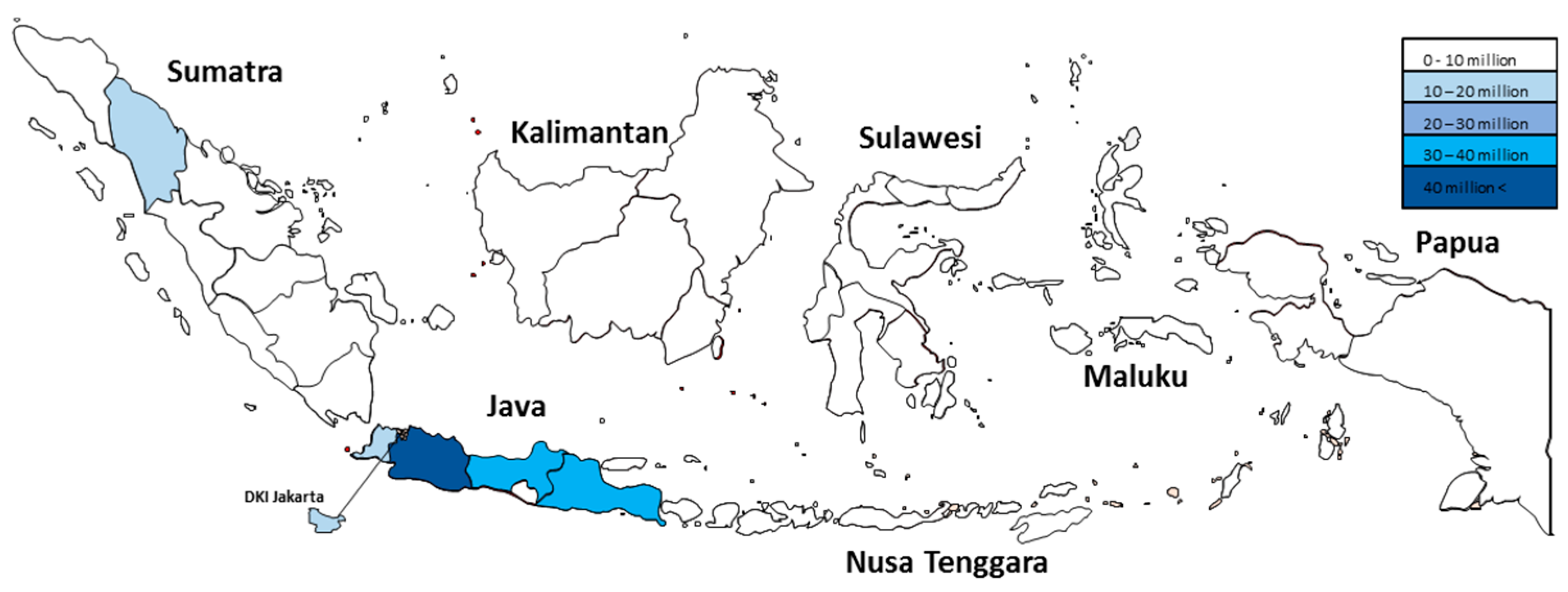
2.1. Provinces of Indonesia
2.2. Input Data
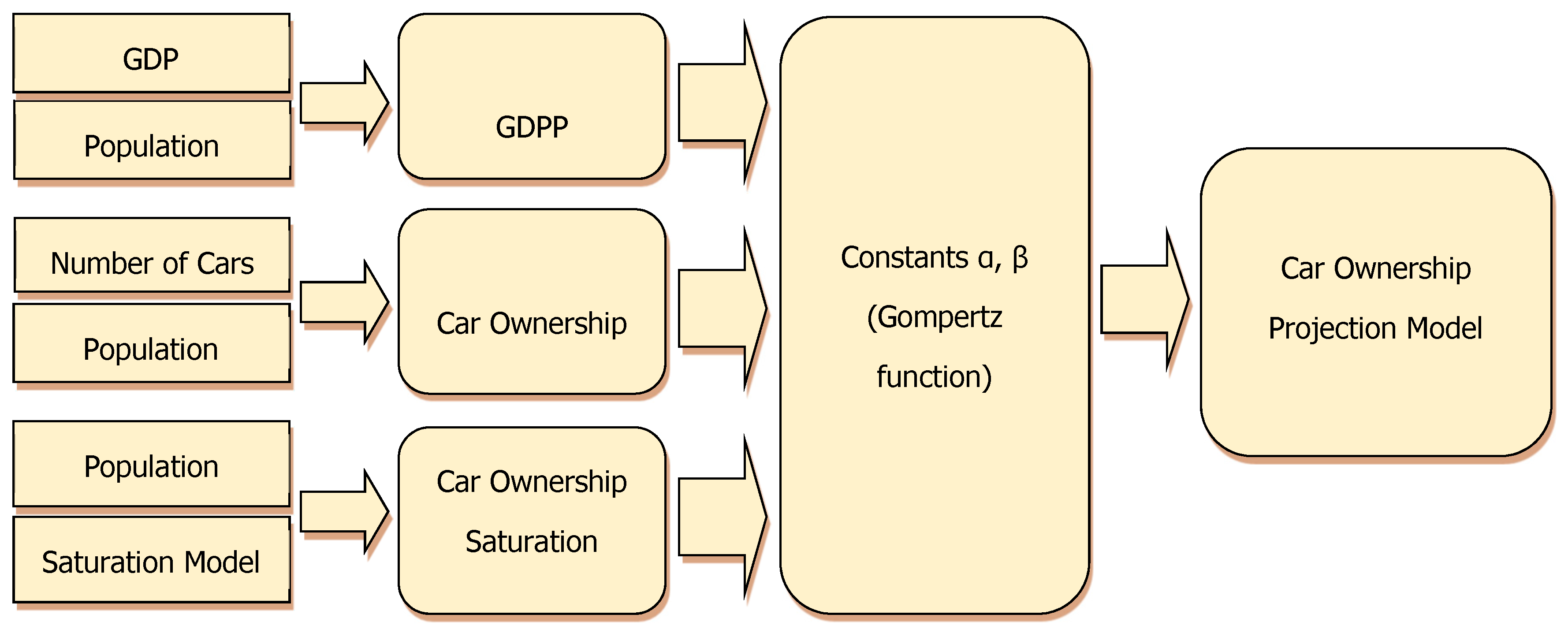
2.3. Car Ownership
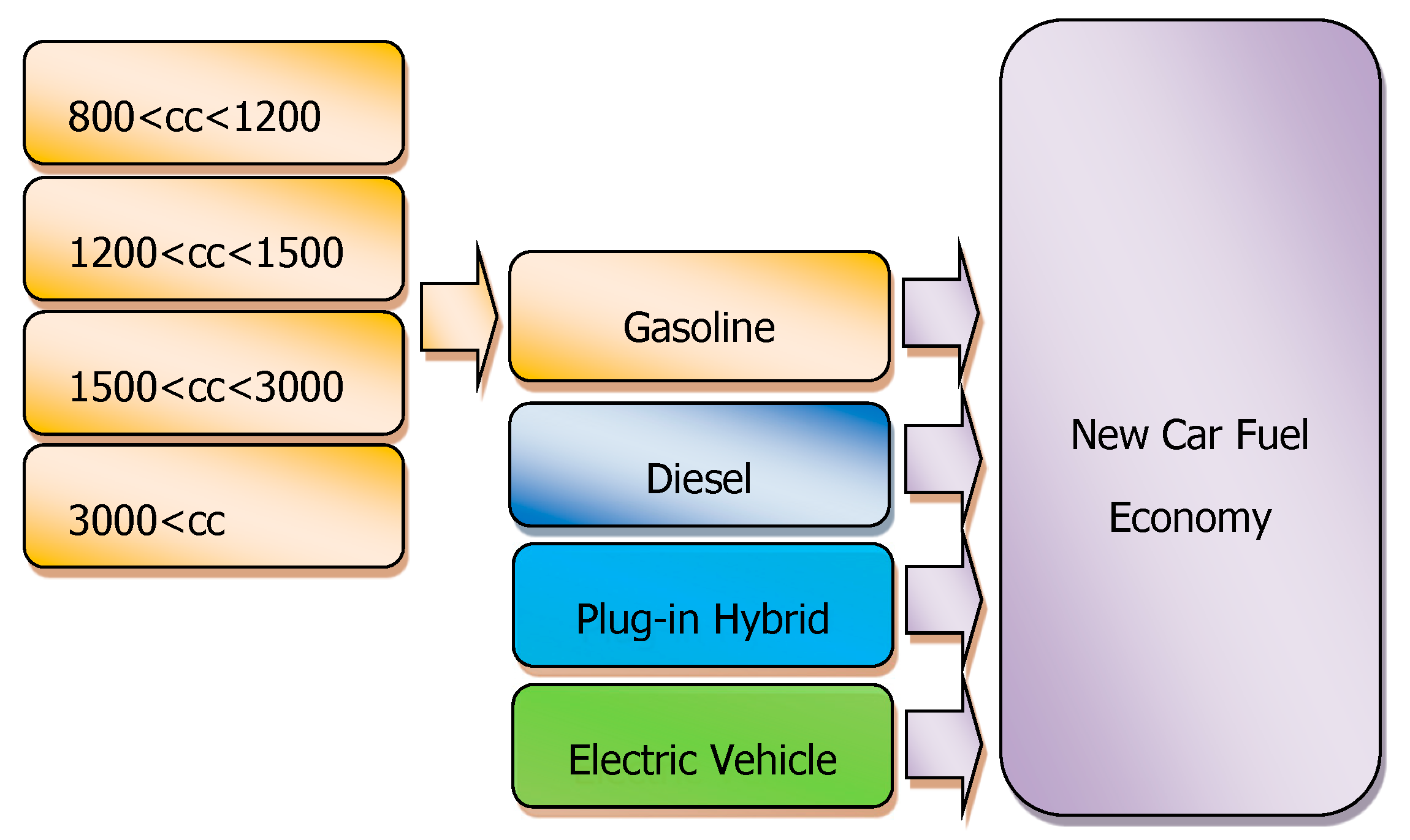
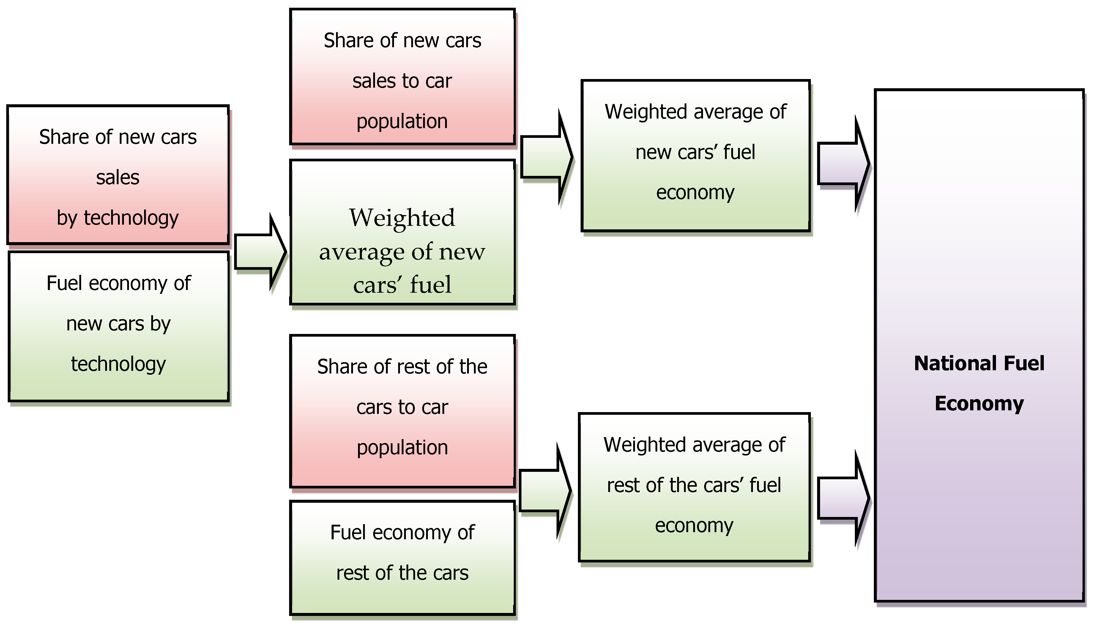
2.4. Car Fuel Economy
2.5. Vehicle Kilometers Traveled
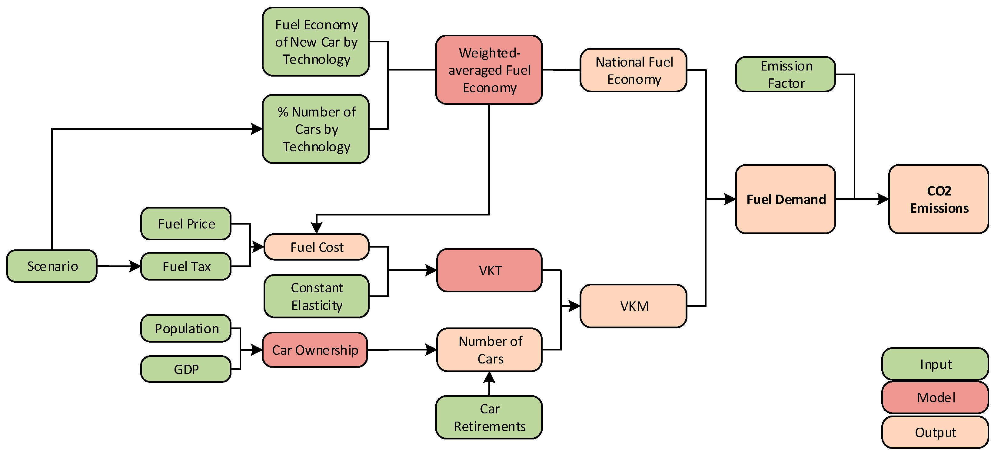
2.6. Energy Demand and CO2 Emissions
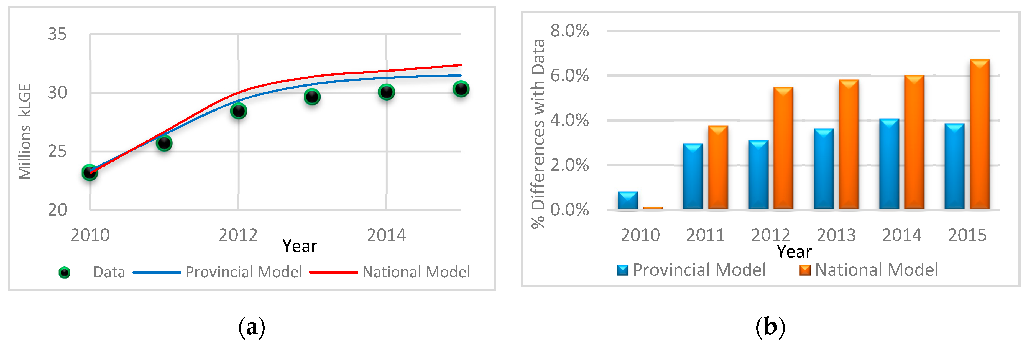
2.7. Model Validation
2.8. Scenarios
3. Results and Discussion
3.1. Historical Results
3.1.1. GDP Per Capita
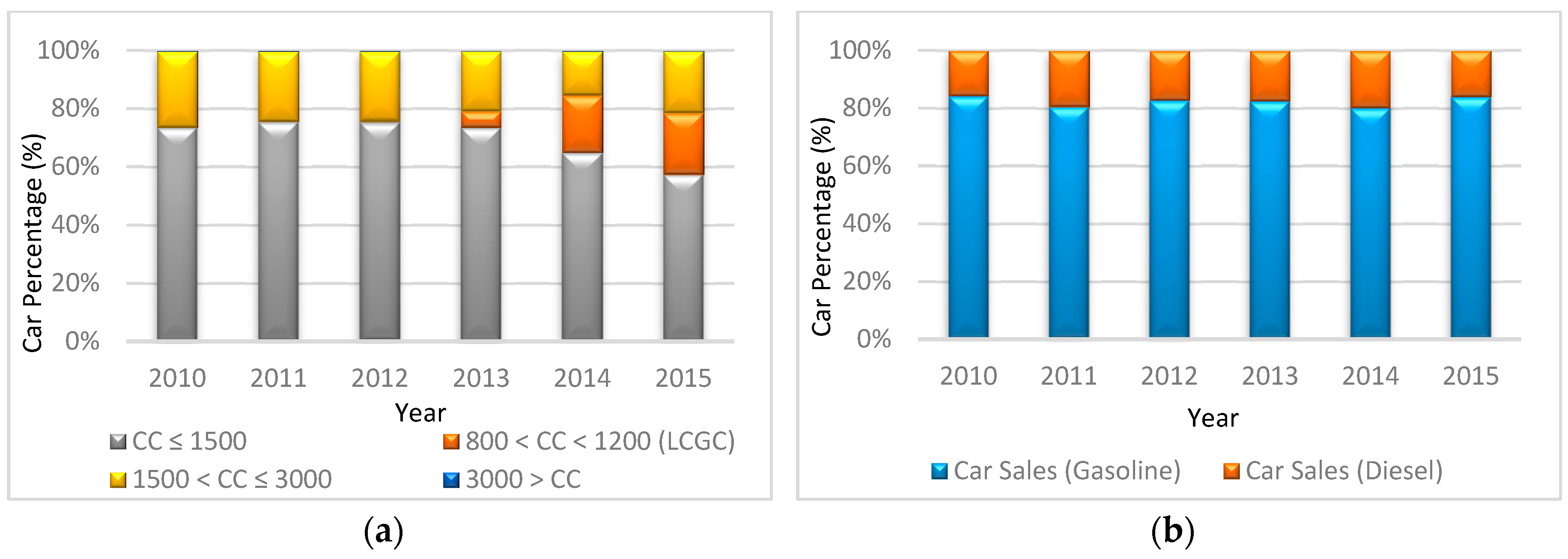
3.1.2. Car Ownership
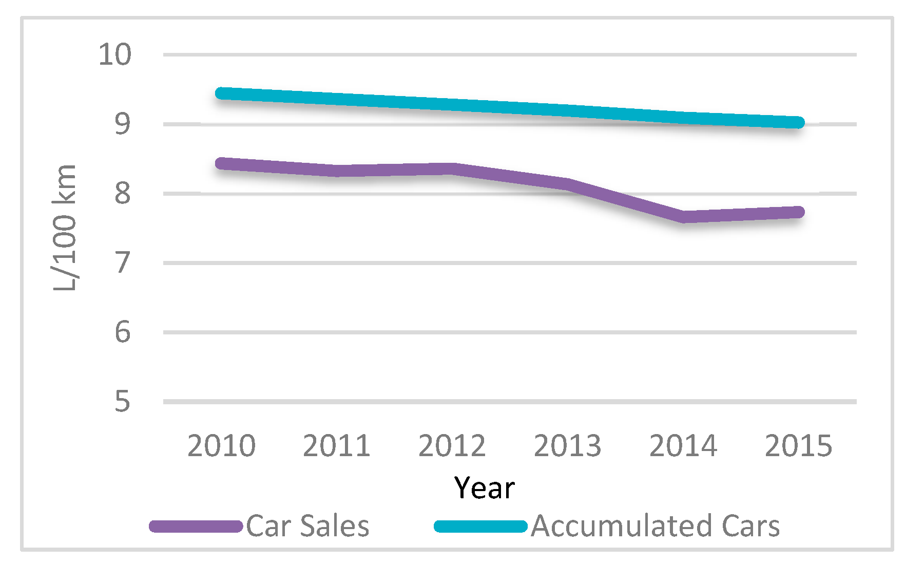
3.1.3. National Car Fuel Economy
3.1.4. Vehicle Kilometers Traveled
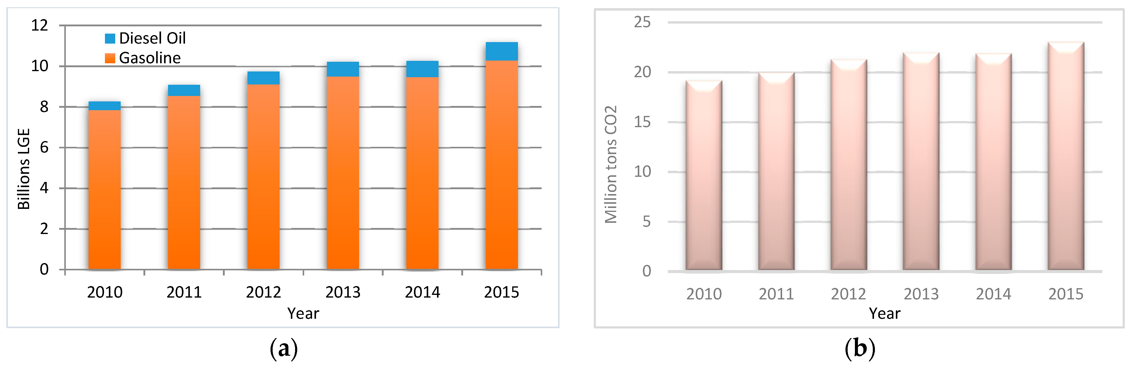
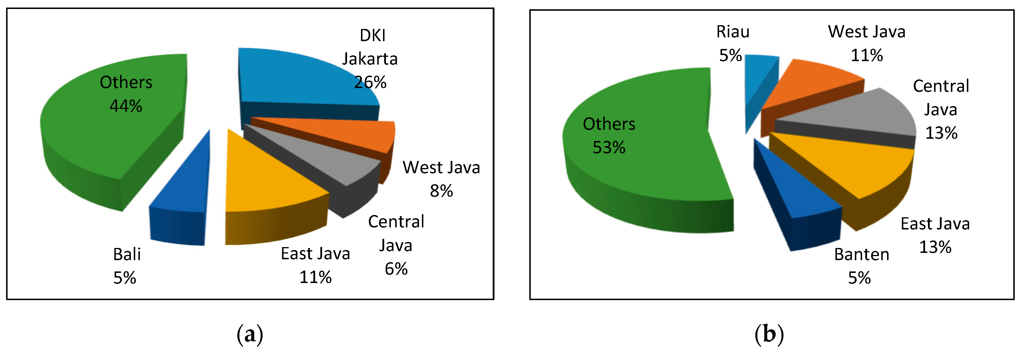
3.1.5. Energy Demand and CO2 Emissions
3.1.6. Model Validation
3.2. Projection Results
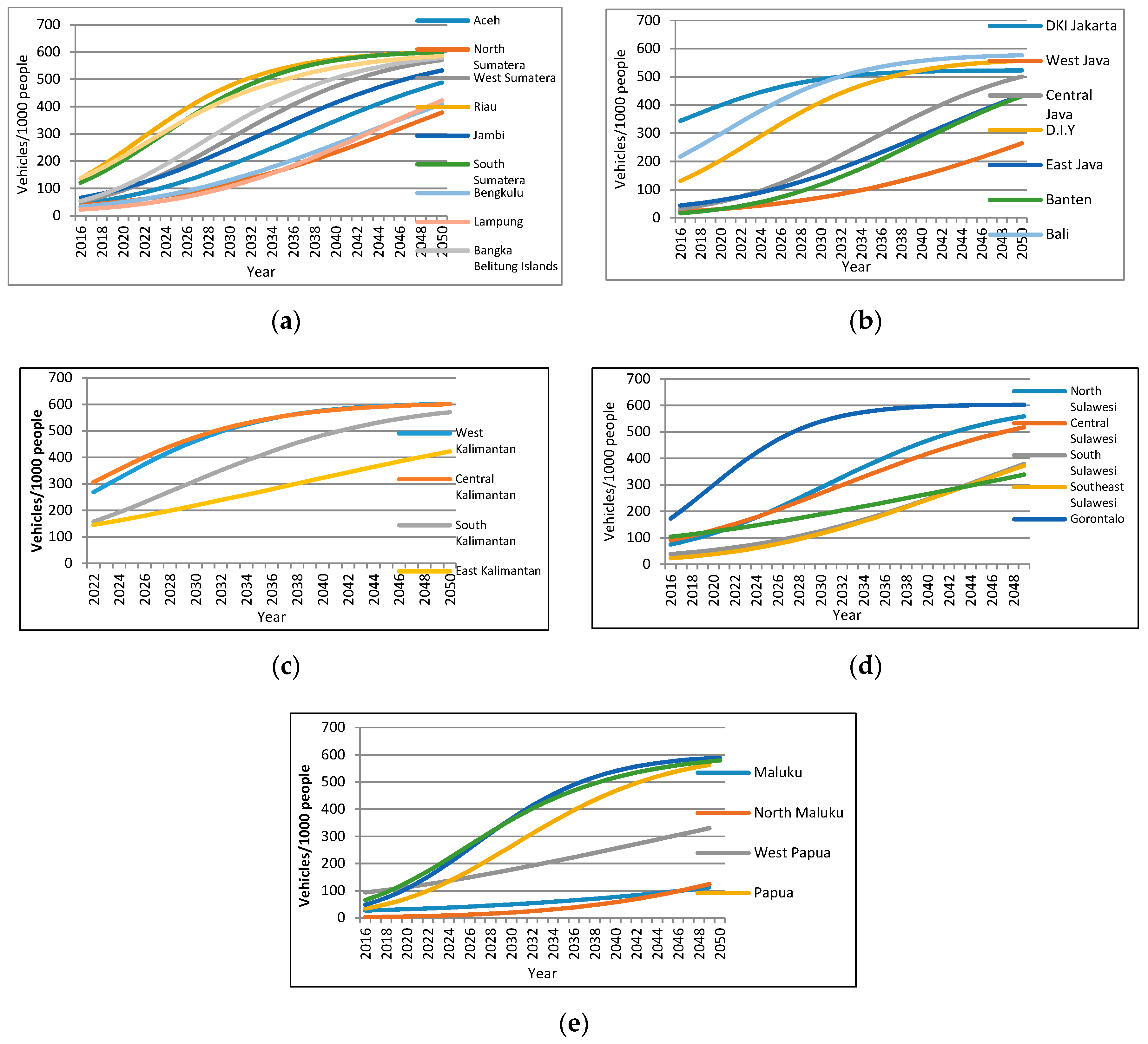
3.2.1. Projection of Car Ownership
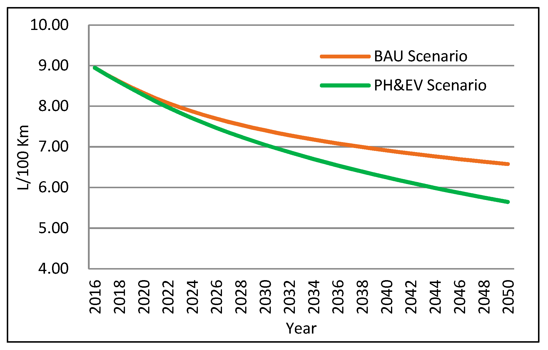
3.2.2. Impact of Policy Scenario
4. Conclusions
Author Contributions
Funding
Conflicts of Interest
Nomenclature
| BOE | Barrel oil equivalent |
| ASIF | Activity Structure Intensity Fuel |
| LCGC | Low Cost Green Car |
| CO | car ownership |
| CO* | saturated car ownership |
| GDPP | GDP per capita |
| D | population density |
| FE | fuel economy |
| FC | fuel cost |
| VKT | vehicle kilometer traveled |
| VKM | vehicle kilometers |
| ԑ | elasticity |
| EF | emission factor |
| E | energy demand |
| G | CO2 emission |
References
- Ministry of Energy and Mineral Resources Republic of Indonesia. Handbook of Energy & Economic Statistics of Indonesia, Head of Center for Energy and Mineral Resources Data and Information; Ministry of Energy and Mineral Resources Republic of Indonesia: Jakarta, Indonesia, 2016.
- Erahman, Q.F.; Purwanto, W.W.; Sudibandriyo, M.; Hidayatno, A. An assessment of Indonesia’s energy security index and comparison with seventy countries. Energy 2016, 111, 364–376. [Google Scholar] [CrossRef]
- Dargay, J.; Gately, D. Vehicle ownership to 2015: Implications for energy use and emissions. Energy Policy 1997, 25, 1121–1127. [Google Scholar] [CrossRef]
- Dargay, J.; Gately, D. Income’s effect on car and vehicle ownership, worldwide: 1960–2015. Transp. Res. Part A Policy Pract. 1999, 33, 101–138. [Google Scholar] [CrossRef]
- Dargay, J.; Gately, D. Modelling global vehicle ownership. In Proceedings of the Ninth World Conference on Transport Research, Seoul, Korea, 22–27 July 2001. [Google Scholar]
- Dargay, J.; Gately, D.; Sommer, M. Vehicle ownership and income growth, worldwide: 1960–2030. Energy J. 2007, 28, 143. [Google Scholar] [CrossRef]
- Leaver, L.; Samuelson, R.; Leaver, J. Potential for low transport energy use in developing Asian cities through compact urban development. In Proceedings of the Third IAEE Asian Conference, Kyoto, Japan, 20–22 February 2012. [Google Scholar]
- Wu, T.; Zhao, H.; Ou, X. Vehicle ownership analysis based on GDP per capita in China: 1963–2050. Sustainability 2014, 6, 4877–4899. [Google Scholar] [CrossRef]
- Ministry of Environment Republic of Indonesia. President Regulation No.61/2011. 2011. Available online: http://www.bappenas.go.id/files/6413/5228/2167/perpres-indonesia-ok__20111116110726__5.pdf (accessed on 10 December 2017).
- Ministry of Environment Republic of Indonesia. President Regulation No.71/2011. 2011. Available online: http://peraturan.go.id/perpres/nomor-71-tahun-2011-11e44c4f4f4b3a90bde2313232303234.html (accessed on 10 December 2017).
- International Energy Agency. Energy Technology Perspectives; International Energy Agency: Paris, France, 2012. [Google Scholar]
- International Energy Agency. Technology roadmap: Fuel Economy of Road Vehicles; International Energy Agency: Paris, France, 2012. [Google Scholar]
- Zhang, M.; Mu, H.; Li, G.; Ning, Y. Forecasting the transport energy demand based on PLSR method in China. Energy 2009, 34, 1396–1400. [Google Scholar] [CrossRef]
- Lu, I.J.; Lewis, C.; Lin, S.J. The forecast of motor vehicle, energy demand and CO2 emission from Taiwan’s road transportation sector. Energy Policy 2009, 37, 2952–2961. [Google Scholar] [CrossRef]
- Chai, J.; Lu, Q.Y.; Wang, S.Y.; Lai, K.K. Analysis of road transportation energy consumption demand in China. Transp. Res. Part D Transp. Environ. 2016, 48, 112–124. [Google Scholar] [CrossRef]
- Bhattacharyya, S.C. Energy Economics: Concepts, Issues, Markets and Governance; Springer Science & Business Media: Berlin, Germany, 2011. [Google Scholar]
- Eom, J.; Schipper, L. Trends in passenger transport energy use in South Korea. Energy Policy 2010, 38, 3598–3607. [Google Scholar] [CrossRef]
- Ma, L.; Liang, J.; Gao, D.; Sun, J.; Li, Z. The Future Demand of Transportation in China: 2030 Scenario based on a Hybrid Model. Procedia Soc. Behav. Sci. 2012, 54, 428–437. [Google Scholar] [CrossRef]
- Baptista, P.C.; Silva, C.M.; Farias, T.L.; Heywood, J.B. Energy and environmental impacts of alternative pathways for the Portuguese road transportation sector. Energy Policy 2012, 51, 802–815. [Google Scholar] [CrossRef]
- Ko, A.; Myung, C.L.; Park, S.; Kwon, S. Scenario-based CO2 emissions reduction potential and energy use in Republic of Korea’s passenger vehicle fleet. Transp. Res. Part A Policy Pract. 2014, 59, 346–356. [Google Scholar] [CrossRef]
- Widyaparaga, A.; Sopha, B.M.; Budiman, A.; Muthohar, I.; Setiawan, I.C.; Lindasista, A.; Soemardjito, J.; Oka, K. Scenarios analysis of energy mix for road transportation sector in Indonesia. Renew. Sustain. Energy Rev. 2017, 70, 13–23. [Google Scholar]
- Central Statistics Bureau Indonesia. Statistik Nasional. 2013. Available online: http://www.bps.go.id/menutab.php?tabel=1&kat=2&id_subyek=17 (accessed on 25 November 2017).
- Gabungan Industri Kendaraan Bermotor. Gaikindo Website. 2017. Available online: www.gaikindo.or.id (accessed on 25 November 2017).
- Central Statistics Bureau Indonesia. Proyeksi Penduduk Menurut Provinsi. 2017. Available online: https://www.bps.go.id/linkTabelStatis/view/id/1274 (accessed on 25 November 2017).
- Central Statistics Bureau Indonesia. Statistik Indonesia: Statistical Yearbook of Indonesia; Biro Pusat Statistik: Jakarta, Indonesia, 2016.
- Ministry of Industry Republic of Indonesia. Minister of Industry Regulation No.33/M-IND/PER/7/2013; Ministry of Industry Republic of Indonesia: Jakarta, Indonesia, 2013.
- Ministry of Industry Republic of Indonesia. Press Conference. 2013. Available online: http://www.kemenperin.go.id/artikel/6775/Menperin-Keluarkan-Peraturan-Mobil-LCGC (accessed on 10 December 2017).
- Automobile Catalog. 2012 Daihatsu Xenia Xi (Model for Asia) Specifications & Performance Data Review. 2017. Available online: http://www.automobile-catalog.com/car/2012/1223810/daihatsu_xenia_xi.html (accessed on 17 October 2017).
- Auto-data.net. Toyota Innova Fuel Economy. 2017. Available online: https://www.auto-data.net/en/?f=showCar&car_id=3435 (accessed on 17 October 2017).
- Australia, C.O. GreenVehicleGuide. Available online: https://www.greenvehicleguide.gov.au/ (accessed on 20 October 2017).
- International Energy Agency. International Comparison of Light-Duty Vehicle Fuel Economy: Evolution Over 8 Years from 2005 to 2013; International Energy Agency: Paris, France, 2014. [Google Scholar]
- International Energy Agency. Transport, Energy and CO2: Moving Towards Sustainability; International Energy Agency: Paris, France, 2009; p. 44. [Google Scholar]
- International Energy Agency. Fuel Economy Policies Implementation Tool (FEPIT); International Energy Agency: Paris, France, 2015. [Google Scholar]
- U.S. Energy Information Administration. Analysis & Projections of Petroleum Prices. 2017. Available online: https://www.eia.gov/analysis/projection-data.cfm#annualproj (accessed on 25 October 2017).
- Stratas Advisors. Global Refining Outlook: 2016–2035. 2016. Available online: https://stratasadvisors.com/~/media/Marketing%20Images/Newsroom%20Items/GlobalRefiningOutlook_Webinar_March10_2016.pdf?la=en (accessed on 15 October 2017).
- Ministry of Energy and Mineral Resources Republic of Indonesia. MEMR Regulation No.1713 K/12 MEM/2012; Ministry of Energy and Mineral Resources: Central Jakarta, Indonesia, 2012.
- Ministry of Environment Republic of Indonesia. Guidelines of National Greenhouse Gas Inventories. 2012. Available online: http://www.kemenperin.go.id/download/11219 (accessed on 10 December 2017).
- Ministry of Energy and Mineral Resources Republic of Indonesia. Faktor Emisi Pembangkit Listrik Sistem Interkoneksi. 2016. Available online: http://www.djk.esdm.go.id/pdf/Faktor%20Emisi%20Pembangkit%20Listrik/Faktor%20Emisi%20Pembangkit%20Listrik%20Tahun%202011-2014.pdf (accessed on 10 December 2017).
- International Energy Agency. Transport energy efficiency; International Energy Agency: Paris, France, 2010. [Google Scholar]
- Secretariat of Cabinet Republic Indonesia. President Regulation No.22/2017; Secretariat of Cabinet Republic Indonesia: Jakarta, Indonesia, 2017. [Google Scholar]
- International Energy Agency. Technology Roadmap: Electric and Plug-in Hybrid Electric Vehicles; International Energy Agency: Paris, France, 2011. [Google Scholar]
- Preece, R. Excise taxation of key commodities across South East Asia: A comparative analysis ahead of the ASEAN Economic Community in 2015. World Cust. J. 2012, 6, 3–16. [Google Scholar]
- Ministry of Energy and Mineral Resources Republic of Indonesia. MEMR Regulation No.32/2008. 2008. Available online: http://prokum.esdm.go.id/permen/2008/permen-esdm-32-2008.pdf (accessed on 10 December 2017).
- Ministry of Energy and Mineral Resources Republic of Indonesia. MEMR Regulation No.25/2013. 2013. Available online: http://prokum.esdm.go.id/permen/2013/Permen%20ESDM%2025%202013.pdf (accessed on 10 December 2017).
- Façanha, C.; Blumberg, K.; Miller, J. Global Transportation Energy and Climate Roadmap; The International Council for Clean Transportation: Washington, DC, USA, 2012. [Google Scholar]
- Cheah, L.; Heywood, J. Meeting, U.S. passenger vehicle fuel economy standards in 2016 and beyond. Energy Policy 2011, 39, 454–466. [Google Scholar] [CrossRef]


| Region | Province | Region | Province |
|---|---|---|---|
| Sumatra | Aceh | Kalimantan | West Kalimantan |
| North Sumatra | Central Kalimantan | ||
| West Sumatra | South Kalimantan | ||
| Riau | East Kalimantan | ||
| Jambi | Sulawesi | North Sulawesi | |
| South Sumatra | Central Sulawesi | ||
| Bengkulu | South Sulawesi | ||
| Lampung | Southeast Sulawesi | ||
| Bangka Belitung Islands | Gorontalo | ||
| Riau Islands | West Sulawesi | ||
| Java | DKI Jakarta | Nusa Tenggara–Maluku–Papua | West Nusa Tenggara |
| West Java | East Nusa Tenggara | ||
| Central Java | Maluku | ||
| D.I.Y | North Maluku | ||
| East Java | West Papua | ||
| Banten | Papua | ||
| Bali |
| Type of Car Technology | BAU Scenario (%) | Car Technology Scenario (%) | ||||||
|---|---|---|---|---|---|---|---|---|
| 2020 | 2030 | 2040 | 2050 | 2020 | 2030 | 2040 | 2050 | |
| Regular Gasoline | 83 | 83 | 83 | 83 | 78 | 68 | 48 | 33 |
| Diesel | 17 | 17 | 17 | 17 | 17 | 17 | 17 | 17 |
| Plug-in Hybrid (PH) | 0 | 0 | 0 | 0 | 5 | 10 | 25 | 35 |
| Electric Vehicle (EV) | 0 | 0 | 0 | 0 | 0 | 5 | 10 | 15 |
| Scenario | Annual Rate of Fuel Economy Improvement | Target Share of Car Sales to Total Car Sales in 2050 | Fuel Tax Rate | |
|---|---|---|---|---|
| Business as Usual (BAU) | Gasoline and Diesel Car 0.09% | No Change | 15% | |
| Car Technology | PH/EV | Gasoline, Diesel, PH/EV Car 0.09%; 0.09%; 1.40% | 50% of PH/EV | 15% |
| Fuel Taxes | Tax 30% | Gasoline and Diesel Car 0.09% | No Change | 30% |
| No. | Province | GDP Per Capita (Rp) | Annual Growth | |||
|---|---|---|---|---|---|---|
| 2000 | 2005 | 2010 | 2015 | |||
| 1 | Aceh | 4,995,043 | 5,568,355 | 6,427,395 | 8,208,249 | 4.29% |
| 2 | North Sumatra | 5,936,151 | 7,136,919 | 9,112,107 | 11,435,561 | 6.18% |
| 3 | West Sumatra | 5,387,147 | 6,411,608 | 7,987,615 | 10,095,631 | 5.83% |
| 4 | Riau | 14,034,330 | 15,108,162 | 17,531,364 | 18,746,113 | 2.24% |
| 5 | Jambi | 3,964,314 | 4,583,988 | 5,622,244 | 7,397,381 | 5.77% |
| 6 | South Sumatra | 5,988,369 | 6,917,533 | 8,535,492 | 10,555,139 | 5.08% |
| 7 | Bengkulu | 3,105,780 | 3,801,072 | 4,842,777 | 6,010,136 | 6.23% |
| 8 | Lampung | 3,448,223 | 4,097,222 | 5,028,805 | 6,344,406 | 5.60% |
| 9 | Bangka Belitung Islands | 7,168,132 | 7,949,017 | 8,709,608 | 10,456,111 | 3.06% |
| 10 | Riau Islands | 18,395,851 | 22,344,514 | 24,265,039 | 28,706,274 | 3.74% |
| 11 | DKI Jakarta | 27,160,473 | 32,812,888 | 41,037,969 | 52,793,584 | 6.29% |
| 12 | West Java | 5,484,062 | 6,165,875 | 7,454,209 | 9,245,740 | 4.57% |
| 13 | Central Java | 3,672,917 | 4,497,646 | 5,763,579 | 7,399,348 | 6.76% |
| 14 | D.I.Y | 4,317,566 | 5,140,272 | 6,068,938 | 7,463,150 | 4.86% |
| 15 | East Java | 5,842,889 | 7,110,540 | 9,111,499 | 12,144,534 | 7.19% |
| 16 | Banten | 6,535,249 | 7,187,098 | 8,284,732 | 9,923,154 | 3.46% |
| 17 | Bali | 5,702,601 | 6,227,553 | 7,391,742 | 9,499,575 | 4.44% |
| 18 | West Nusa Tenggara | 3,041,105 | 3,568,679 | 4,444,685 | 4,713,600 | 3.67% |
| 19 | East Nusa Tenggara | 1,992,050 | 2,285,129 | 2,666,020 | 3,214,568 | 4.09% |
| 20 | West Kalimantan | 4,803,628 | 5,533,075 | 6,875,073 | 8,405,443 | 5.00% |
| 21 | Central Kalimantan | 5,944,899 | 6,898,169 | 8,467,974 | 10,404,069 | 5.00% |
| 22 | South Kalimantan | 6,266,482 | 7,045,690 | 8,421,300 | 10,107,667 | 4.09% |
| 23 | East Kalimantan | 12,325,552 | 14,314,410 | 18,747,036 | 32,503,297 | 10.91% |
| 24 | North Sulawesi | 5,295,832 | 5,951,651 | 8,068,150 | 10,711,207 | 6.82% |
| 25 | Central Sulawesi | 3,977,784 | 4,940,970 | 6,660,685 | 8,922,062 | 8.29% |
| 26 | South Sulawesi | 3,506,238 | 4,526,019 | 6,352,030 | 8,623,764 | 9.73% |
| 27 | Southeast Sulawesi | 3,170,649 | 3,960,096 | 5,194,289 | 6,794,659 | 7.62% |
| 28 | Gorontalo | 1,764,308 | 2,162,664 | 2,792,392 | 3,668,652 | 7.20% |
| 29 | West Sulawesi | 1,076,863 | 3,030,552 | 4,073,206 | 5,507,867 | 27.43% |
| 30 | Maluku | 2,297,113 | 2,379,840 | 2,757,219 | 3,436,217 | 3.31% |
| 31 | North Maluku | 2,394,251 | 2,453,784 | 2,909,660 | 3,526,332 | 3.15% |
| 32 | West Papua | 1,238,184 | 8,227,709 | 12,232,275 | 19,351,973 | 97.53% |
| 33 | Papua | 6,013,255 | 6,968,230 | 8,195,795 | 8,575,849 | 2.84% |
| No. | Province | 2000 | 2005 | 2010 | 2015 |
|---|---|---|---|---|---|
| 1 | Aceh | 6 | 15 | 21 | 31 |
| 2 | North Sumatra | 14 | 18 | 25 | 36 |
| 3 | West Sumatra | 6 | 8 | 24 | 43 |
| 4 | Riau | 10 | 40 | 80 | 100 |
| 5 | Jambi | 9 | 17 | 30 | 51 |
| 6 | South Sumatra | 8 | 21 | 51 | 87 |
| 7 | Bengkulu | 7 | 10 | 19 | 27 |
| 8 | Lampung | 6 | 9 | 10 | 20 |
| 9 | Bangka Belitung Islands | 5 | 8 | 17 | 41 |
| 10 | Riau Islands | 10 | 28 | 73 | 93 |
| 11 | DKI Jakarta | 148 | 196 | 242 | 345 |
| 12 | West Java | 9 | 11 | 13 | 21 |
| 13 | Central Java | 6 | 6 | 13 | 25 |
| 14 | D.I.Y | 21 | 32 | 72 | 99 |
| 15 | East Java | 12 | 20 | 27 | 37 |
| 16 | Banten | 2 | 3 | 8 | 12 |
| 17 | Bali | 34 | 97 | 134 | 170 |
| 18 | West Nusa Tenggara | 3 | 7 | 23 | 31 |
| 19 | East Nusa Tenggara | 2 | 8 | 29 | 36 |
| 20 | West Kalimantan | 6 | 20 | 65 | 78 |
| 21 | Central Kalimantan | 3 | 26 | 83 | 101 |
| 22 | South Kalimantan | 11 | 24 | 43 | 58 |
| 23 | East Kalimantan | 15 | 30 | 56 | 71 |
| 24 | North Sulawesi | 11 | 16 | 32 | 65 |
| 25 | Central Sulawesi | 9 | 35 | 54 | 68 |
| 26 | South Sulawesi | 8 | 15 | 22 | 32 |
| 27 | Southeast Sulawesi | 1 | 4 | 9 | 17 |
| 28 | Gorontalo | 0 | 5 | 63 | 85 |
| 29 | West Sulawesi | 35 | 54 | 72 | 99 |
| 30 | Maluku | 16 | 20 | 21 | 27 |
| 31 | North Maluku | 1 | 1 | 1 | 3 |
| 32 | West Papua | 18 | 29 | 68 | 92 |
| 33 | Papua | 5 | 8 | 20 | 28 |
| No | Province | Pop. Density (Pop/Ha) | α | β | CO* (Vehicles/1000 People) | R2 |
|---|---|---|---|---|---|---|
| 1 | Aceh | 0.76 | −8.2 | −0.00000013 | 603.31 | 0.877 |
| 2 | North Sumatra | 1.77 | −5.0 | −0.00000005 | 599.06 | 0.997 |
| 3 | West Sumatra | 1.11 | −10.0 | −0.00000013 | 601.82 | 0.943 |
| 4 | Riau | 0.62 | −36.7 | −0.00000017 | 603.91 | 0.915 |
| 5 | Jambi | 0.58 | −7.5 | −0.00000016 | 604.06 | 0.919 |
| 6 | South Sumatra | 0.85 | −12.3 | −0.00000018 | 602.93 | 0.937 |
| 7 | Bengkulu | 0.85 | −6.8 | −0.00000013 | 602.92 | 0.951 |
| 8 | Lampung | 2.14 | −6.7 | −0.00000011 | 597.53 | 0.977 |
| 9 | Bangka Belitung Islands | 0.70 | −21.4 | −0.00000020 | 603.59 | 0.930 |
| 10 | Riau Islands | 1.43 | −24.9 | −0.00000010 | 600.57 | 0.791 |
| 11 | DKI Jakarta | 21.28 | −3.5 | −0.00000004 | 523.08 | 0.973 |
| 12 | West Java | 11.12 | −5.7 | −0.00000006 | 561.47 | 0.974 |
| 13 | Central Java | 9.91 | −7.9 | −0.00000013 | 565.96 | 0.957 |
| 14 | D.I.Y | 10.63 | −9.1 | −0.00000023 | 563.25 | 0.917 |
| 15 | East Java | 7.63 | −5.0 | −0.00000005 | 575.06 | 0.884 |
| 16 | Banten | 10.38 | −11.8 | −0.00000012 | 564.55 | 0.905 |
| 17 | Bali | 6.55 | −6.9 | −0.00000020 | 579.55 | 0.697 |
| 18 | West Nusa Tenggara | 2.18 | −18.0 | −0.00000040 | 597.36 | 0.899 |
| 19 | East Nusa Tenggara | 0.94 | −18.3 | −0.00000063 | 602.56 | 0.804 |
| 20 | West Kalimantan | 0.30 | −14.5 | −0.00000025 | 605.25 | 0.813 |
| 21 | Central Kalimantan | 0.14 | −19.1 | −0.00000025 | 605.91 | 0.799 |
| 22 | South Kalimantan | 0.93 | −9.1 | −0.00000014 | 602.62 | 0.870 |
| 23 | East Kalimantan | 0.17 | −4.5 | −0.00000003 | 605.81 | 0.651 |
| 24 | North Sulawesi | 1.52 | −6.8 | −0.00000011 | 600.12 | 0.969 |
| 25 | Central Sulawesi | 0.41 | −5.9 | −0.00000012 | 604.77 | 0.721 |
| 26 | South Sulawesi | 1.77 | −5.2 | −0.00000007 | 599.07 | 0.867 |
| 27 | Southeast Sulawesi | 0.56 | −9.5 | −0.00000015 | 604.14 | 0.955 |
| 28 | Gorontalo | 0.79 | −30.9 | −0.00000084 | 603.17 | 0.826 |
| 29 | West Sulawesi | 0.64 | −3.3 | −0.00000011 | 603.80 | 0.951 |
| 30 | Maluku | 0.23 | −4.2 | −0.00000009 | 605.53 | 0.850 |
| 31 | North Maluku | 0.30 | −10.4 | −0.00000018 | 605.22 | 0.928 |
| 32 | West Papua | 0.07 | −4.0 | −0.00000004 | 606.21 | 0.825 |
| 33 | Papua | 0.08 | −17.0 | −0.00000020 | 606.14 | 0.949 |
| No. | Province | 2012 | 2013 | 2014 | 2015 | Elasticity |
|---|---|---|---|---|---|---|
| 1 | Aceh | 8902 | 7867 | 7113 | 6647 | −0.646 |
| 2 | North Sumatra | 11,962 | 11,319 | 10,822 | 10,499 | −0.288 |
| 3 | West Sumatra | 15,432 | 13,916 | 12,791 | 12,085 | −0.541 |
| 4 | Riau | 9623 | 9142 | 8768 | 8525 | −0.268 |
| 5 | Jambi | 5827 | 5182 | 4710 | 4416 | −0.613 |
| 6 | South Sumatra | 6799 | 6110 | 5600 | 5281 | −0.559 |
| 7 | Bengkulu | 10,242 | 9574 | 9062 | 8733 | −0.352 |
| 8 | Lampung | 16,858 | 15,591 | 14,629 | 14,014 | −0.409 |
| 9 | Bangka Belitung Islands | 17,743 | 15,363 | 13,660 | 12,621 | −0.753 |
| 10 | Riau Islands | 10,563 | 9909 | 9406 | 9082 | −0.334 |
| 11 | DKI Jakarta | 4762 | 4334 | 4013 | 3811 | −0.492 |
| 12 | West Java | 33,674 | 31,320 | 29,523 | 28,371 | −0.379 |
| 13 | Central Java | 10,753 | 10,106 | 9608 | 9286 | −0.324 |
| 14 | D.I.Y | 5231 | 4638 | 4204 | 3935 | −0.629 |
| 15 | East Java | 10,641 | 10,024 | 9547 | 9239 | −0.313 |
| 16 | Banten | 48,432 | 44,062 | 40,793 | 38,728 | −0.494 |
| 17 | Bali | 6612 | 5917 | 5404 | 5084 | −0.581 |
| 18 | West Nusa Tenggara | 8213 | 7953 | 7748 | 7612 | −0.168 |
| 19 | East Nusa Tenggara | 6994 | 6594 | 6285 | 6085 | −0.308 |
| 20 | West Kalimantan | 7740 | 7131 | 6671 | 6378 | −0.428 |
| 21 | Central Kalimantan | 7889 | 7311 | 6872 | 6590 | −0.398 |
| 22 | South Kalimantan | 10,001 | 9326 | 8810 | 8478 | −0.365 |
| 23 | East Kalimantan | 10,525 | 8608 | 7307 | 6543 | −1.051 |
| 24 | North Sulawesi | 10,696 | 9600 | 8791 | 8284 | −0.565 |
| 25 | Central Sulawesi | 5368 | 4874 | 4506 | 4273 | −0.504 |
| 26 | South Sulawesi | 18,582 | 18,108 | 17,730 | 17,479 | −0.135 |
| 27 | Southeast Sulawesi | 8336 | 7906 | 7573 | 7356 | −0.276 |
| 28 | Gorontalo | 9325 | 8642 | 8122 | 7789 | −0.398 |
| 29 | West Sulawesi | 3945 | 3895 | 3854 | 3828 | −0.067 |
| 30 | Maluku | 11,336 | 10,035 | 9085 | 8497 | −0.638 |
| 31 | North Maluku | 38,195 | 35,925 | 34,174 | 33,042 | −0.320 |
| 32 | West Papua | 8690 | 8299 | 7994 | 7794 | −0.241 |
| 33 | Papua | 17,289 | 15,564 | 14,286 | 13,484 | −0.550 |
| No | Province | 2010 | 2011 | 2012 | 2013 | 2014 | 2015 |
|---|---|---|---|---|---|---|---|
| 1 | Aceh | 80,272,962 | 83,459,252 | 96,186,659 | 97,151,788 | 88,041,546 | 92,007,033 |
| 2 | North Sumatera | 368,195,076 | 398,778,700 | 428,807,615 | 433,495,984 | 434,806,571 | 471,777,332 |
| 3 | West Sumatera | 171,715,475 | 191,061,362 | 212,860,361 | 210,369,069 | 231,204,316 | 244,306,713 |
| 4 | Riau | 401,637,066 | 424,232,500 | 459,651,842 | 456,782,973 | 449,075,161 | 488,310,136 |
| 5 | Jambi | 51,014,129 | 57,683,445 | 65,676,461 | 71,232,337 | 65,564,801 | 68,754,473 |
| 6 | South Sumatera | 243,740,412 | 285,420,963 | 309,373,517 | 349,723,175 | 318,295,916 | 335,691,155 |
| 7 | Bengkulu | 30,708,475 | 32,460,514 | 37,205,988 | 39,572,877 | 37,694,000 | 40,625,685 |
| 8 | Lampung | 124,065,421 | 167,065,519 | 189,579,767 | 197,602,219 | 196,189,768 | 210,202,499 |
| 9 | Bangka Belitung Islands | 35,605,535 | 37,772,088 | 62,464,307 | 62,710,826 | 62,720,635 | 64,810,117 |
| 10 | Kepulauan Riau | 122,207,893 | 129,159,132 | 139,937,588 | 141,387,616 | 138,772,831 | 149,853,524 |
| 11 | DKI Jakarta | 1,041,349,357 | 1,128,301,346 | 1,212,311,139 | 1,199,831,839 | 1,153,330,676 | 1,207,272,570 |
| 12 | West Java | 1,733,899,566 | 2,105,777,600 | 2,302,590,272 | 2,435,271,958 | 2,371,599,183 | 2,548,918,144 |
| 13 | Central Java | 427,186,435 | 563,028,914 | 626,886,265 | 658,273,258 | 666,448,449 | 720,390,417 |
| 14 | D.I.Y | 121,431,212 | 128,677,346 | 139,728,931 | 133,105,959 | 124,060,828 | 129,877,218 |
| 15 | East Jawa | 1,011,926,496 | 1,069,281,965 | 1,145,698,694 | 1,128,630,903 | 1,102,302,720 | 1,193,007,164 |
| 16 | Banten | 386,896,273 | 421,268,116 | 454,630,752 | 497,883,116 | 461,856,866 | 490,402,758 |
| 17 | Bali | 323,614,972 | 342,779,339 | 354,166,716 | 328,268,247 | 308,332,155 | 324,423,028 |
| 18 | West Nusa Tenggara | 81,830,739 | 86,357,530 | 90,167,797 | 92,074,655 | 93,458,079 | 102,697,056 |
| 19 | East Nusa Tenggara | 90,600,494 | 95,731,381 | 95,951,047 | 92,317,948 | 92,448,663 | 100,106,854 |
| 20 | West Kalimantan | 208,164,352 | 220,190,058 | 223,421,205 | 208,194,952 | 201,069,751 | 214,994,820 |
| 21 | Central Kalimantan | 136,805,275 | 144,669,366 | 148,016,116 | 143,807,128 | 139,959,792 | 150,126,893 |
| 22 | South Kalimantan | 146,094,739 | 154,448,564 | 168,224,184 | 165,499,922 | 163,589,675 | 176,070,648 |
| 23 | East Kalimantan | 194,524,071 | 206,911,074 | 222,905,541 | 193,585,308 | 169,301,566 | 169,552,498 |
| 24 | North Sulawesi | 73,766,474 | 78,123,605 | 84,540,991 | 118,237,705 | 111,633,930 | 117,658,795 |
| 25 | Central Sulawesi | 71,377,751 | 75,552,719 | 77,884,330 | 72,505,069 | 70,734,641 | 75,027,803 |
| 26 | South Sulawesi | 312,293,952 | 353,372,892 | 370,622,887 | 393,444,364 | 386,676,987 | 426,360,187 |
| 27 | Southeast Sulawesi | 15,219,392 | 18,787,111 | 21,832,002 | 25,485,292 | 25,825,223 | 28,056,494 |
| 28 | Gorontalo | 58,001,180 | 61,335,857 | 65,203,277 | 61,777,834 | 63,334,762 | 67,934,623 |
| 29 | West Sulawesi | 31,033,577 | 35,094,179 | 36,785,788 | 39,566,758 | 39,304,488 | 43,651,669 |
| 30 | Maluku | 35,038,104 | 37,132,142 | 38,651,965 | 35,763,610 | 32,921,279 | 34,434,362 |
| 31 | North Maluku | 4,312,530 | 4,543,853 | 6,847,329 | 8,468,084 | 9,045,675 | 9,782,882 |
| 32 | West Papua | 42,763,281 | 45,158,205 | 46,431,041 | 46,741,345 | 51,636,318 | 56,308,624 |
| 33 | Papua | 93,191,714 | 98,682,995 | 101,732,042 | 96,536,439 | 101,630,751 | 107,288,022 |
| Indonesia | 8,270,484,380 | 9,282,299,634 | 10,036,974,419 | 10,235,300,557 | 9,962,867,999 | 10,660,682,198 | |
| No | Province | 2016 | 2020 | 2030 | 2040 | 2050 |
|---|---|---|---|---|---|---|
| 1 | Aceh | 1332 | 1701 | 4128 | 6749 | 8285 |
| 2 | North Sumatera | 5125 | 6406 | 13,544 | 23,550 | 33,210 |
| 3 | West Sumatera | 2964 | 4406 | 11,910 | 17,758 | 19,007 |
| 4 | Riau | 6887 | 10,596 | 20,416 | 22,872 | 21,605 |
| 5 | Jambi | 900 | 1138 | 2534 | 3770 | 4279 |
| 6 | South Sumatera | 4717 | 6533 | 13,263 | 15,422 | 14,630 |
| 7 | Bengkulu | 499 | 667 | 1603 | 2829 | 3833 |
| 8 | Lampung | 2353 | 3192 | 8688 | 17,472 | 25,492 |
| 9 | Bangka Belitung Islands | 861 | 1320 | 3537 | 4797 | 4901 |
| 10 | Riau Islands | 2291 | 3211 | 6062 | 7035 | 6842 |
| 11 | DKI Jakarta | 12,181 | 12,428 | 15,171 | 14,914 | 13,635 |
| 12 | West Java | 27,079 | 33,387 | 72,478 | 131,456 | 198,790 |
| 13 | Central Java | 9183 | 14,281 | 42,067 | 73,286 | 87,673 |
| 14 | D.I.Y | 1726 | 2199 | 4119 | 4763 | 4560 |
| 15 | East Java | 14,251 | 18,439 | 41,458 | 70,599 | 92,029 |
| 16 | Banten | 7127 | 10,982 | 36,683 | 73,275 | 99,262 |
| 17 | Bali | 4190 | 4825 | 7407 | 7905 | 7391 |
| 18 | West Nusa Tenggara | 1632 | 3249 | 9989 | 13,504 | 13,306 |
| 19 | East Nusa Tenggara | 1875 | 3242 | 8277 | 10,790 | 10,870 |
| 20 | West Kalimantan | 3592 | 5197 | 10,415 | 11,926 | 11,252 |
| 21 | Central Kalimantan | 2523 | 3408 | 6035 | 6717 | 6347 |
| 22 | South Kalimantan | 2418 | 3428 | 7869 | 10,995 | 11,600 |
| 23 | East Kalimantan | 2561 | 2366 | 3658 | 4721 | 5423 |
| 24 | North Sulawesi | 1358 | 1772 | 3999 | 5737 | 6167 |
| 25 | Central Sulawesi | 1023 | 1240 | 2415 | 3366 | 3756 |
| 26 | South Sulawesi | 5192 | 6934 | 15,327 | 26,892 | 37,333 |
| 27 | Southeast Sulawesi | 384 | 574 | 1600 | 2960 | 4066 |
| 28 | Gorontalo | 1398 | 2089 | 3604 | 3708 | 3402 |
| 29 | West Sulawesi | 470 | 554 | 844 | 1095 | 1270 |
| 30 | Maluku | 357 | 352 | 525 | 721 | 950 |
| 31 | North Maluku | 108 | 163 | 546 | 1351 | 2604 |
| 32 | West Papua | 590 | 668 | 1034 | 1358 | 1591 |
| 33 | Papua | 1332 | 2258 | 7260 | 11,323 | 12,256 |
| Indonesia | 130,478 | 173,204 | 388,465 | 615,618 | 777,617 | |
| No | Province | 2016 | 2020 | 2030 | 2040 | 2050 |
|---|---|---|---|---|---|---|
| 1 | Aceh | 119,148,323 | 141,523,449 | 303,607,934 | 461,464,806 | 540,244,217 |
| 2 | North Sumatera | 458,543,142 | 533,014,420 | 996,144,764 | 1,610,238,179 | 2,165,457,146 |
| 3 | West Sumatera | 265,192,718 | 366,591,863 | 875,942,962 | 1,214,204,525 | 1,239,355,128 |
| 4 | Riau | 616,226,815 | 881,589,123 | 1,501,512,434 | 1,563,904,525 | 1,408,724,650 |
| 5 | Jambi | 80,552,871 | 94,647,348 | 186,339,112 | 257,809,352 | 279,043,157 |
| 6 | South Sumatera | 422,063,720 | 543,568,995 | 975,487,176 | 1,054,481,349 | 953,949,811 |
| 7 | Bengkulu | 44,636,584 | 55,464,461 | 117,917,482 | 193,412,673 | 249,924,630 |
| 8 | Lampung | 210,516,097 | 265,594,157 | 638,973,126 | 1,194,670,091 | 1,662,176,551 |
| 9 | Bangka Belitung Islands | 77,063,962 | 109,808,609 | 260,164,030 | 328,000,084 | 319,551,372 |
| 10 | Kepulauan Riau | 204,942,989 | 267,180,562 | 445,877,246 | 481,031,935 | 446,116,423 |
| 11 | DKI Jakarta | 1,089,849,014 | 1,034,018,568 | 1,115,802,771 | 1,019,749,331 | 889,080,510 |
| 12 | West Java | 2,422,887,664 | 2,777,829,389 | 5,330,535,379 | 8,988,375,156 | 12,962,040,540 |
| 13 | Central Java | 821,685,057 | 1,188,229,370 | 3,093,896,625 | 5,010,986,595 | 5,716,720,151 |
| 14 | D.I.Y | 154,409,331 | 182,962,705 | 302,952,178 | 325,705,446 | 297,304,363 |
| 15 | East Jawa | 1,275,065,275 | 1,534,166,702 | 3,049,075,086 | 4,827,280,936 | 6,000,723,531 |
| 16 | Banten | 637,695,462 | 913,691,429 | 2,697,915,219 | 5,010,194,194 | 6,472,332,110 |
| 17 | Bali | 374,879,124 | 401,436,895 | 544,728,515 | 540,503,534 | 481,907,250 |
| 18 | West Nusa Tenggara | 146,061,501 | 270,335,225 | 734,625,142 | 923,360,040 | 867,604,144 |
| 19 | East Nusa Tenggara | 167,767,743 | 269,777,612 | 608,735,560 | 737,792,520 | 708,745,604 |
| 20 | West Kalimantan | 321,358,616 | 432,411,794 | 766,017,330 | 815,450,870 | 733,708,303 |
| 21 | Central Kalimantan | 225,759,254 | 283,570,145 | 443,844,722 | 459,285,481 | 413,845,972 |
| 22 | South Kalimantan | 216,361,886 | 285,199,263 | 578,752,860 | 751,783,980 | 756,379,095 |
| 23 | East Kalimantan | 229,105,517 | 196,859,130 | 269,020,170 | 322,828,260 | 353,611,885 |
| 24 | North Sulawesi | 121,545,236 | 147,408,264 | 294,134,362 | 392,257,298 | 402,148,817 |
| 25 | Central Sulawesi | 91,562,634 | 103,195,605 | 177,637,834 | 230,150,517 | 244,921,880 |
| 26 | South Sulawesi | 464,591,258 | 576,928,440 | 1,127,220,035 | 1,838,777,953 | 2,434,305,858 |
| 27 | Southeast Sulawesi | 34,396,473 | 47,753,362 | 117,644,424 | 202,392,077 | 265,101,108 |
| 28 | Gorontalo | 125,043,868 | 173,800,532 | 265,064,967 | 253,555,081 | 221,825,482 |
| 29 | West Sulawesi | 42,066,227 | 46,053,319 | 62,040,380 | 74,887,606 | 82,830,661 |
| 30 | Maluku | 31,965,517 | 29,320,690 | 38,589,159 | 49,286,590 | 61,960,934 |
| 31 | North Maluku | 9,620,306 | 13,548,369 | 40,155,478 | 92,387,460 | 169,790,491 |
| 32 | West Papua | 52,763,586 | 55,606,413 | 76,011,800 | 92,843,257 | 103,709,345 |
| 33 | Papua | 119,173,052 | 187,851,251 | 533,985,506 | 774,195,128 | 799,173,697 |
| Indonesia | 11.674.500.823 | 14,410,937,457 | 28,570,351,767 | 42,093,246,828 | 50,704,314,820 | |
© 2019 by the authors. Licensee MDPI, Basel, Switzerland. This article is an open access article distributed under the terms and conditions of the Creative Commons Attribution (CC BY) license (http://creativecommons.org/licenses/by/4.0/).
Share and Cite
Erahman, Q.F.; Reyseliani, N.; Purwanto, W.W.; Sudibandriyo, M. Modeling Future Energy Demand and CO2 Emissions of Passenger Cars in Indonesia at the Provincial Level. Energies 2019, 12, 3168. https://doi.org/10.3390/en12163168
Erahman QF, Reyseliani N, Purwanto WW, Sudibandriyo M. Modeling Future Energy Demand and CO2 Emissions of Passenger Cars in Indonesia at the Provincial Level. Energies. 2019; 12(16):3168. https://doi.org/10.3390/en12163168
Chicago/Turabian StyleErahman, Qodri Febrilian, Nadhilah Reyseliani, Widodo Wahyu Purwanto, and Mahmud Sudibandriyo. 2019. "Modeling Future Energy Demand and CO2 Emissions of Passenger Cars in Indonesia at the Provincial Level" Energies 12, no. 16: 3168. https://doi.org/10.3390/en12163168
APA StyleErahman, Q. F., Reyseliani, N., Purwanto, W. W., & Sudibandriyo, M. (2019). Modeling Future Energy Demand and CO2 Emissions of Passenger Cars in Indonesia at the Provincial Level. Energies, 12(16), 3168. https://doi.org/10.3390/en12163168