Performance Enhancement of Micro Grid System with SMES Storage System Based on Mine Blast Optimization Algorithm

Abstract

Frequency control represents a critically significant issue for the enhancement of the dynamic performance of isolated micro grids. The micro grid system studied here was a wind–diesel system. A new and robust optimization technique called the mine blast algorithm (MBA) was designed for tuning the PID (proportional–integral–differential) gains of the blade pitch controller of the wind turbine side and the gains of the superconducting magnetic energy storage (SMES) controller. SMES was implemented to release and absorb active power quickly in order to achieve a balance between generation and load power, and thereby control system frequency. The minimization of frequency and output wind power deviations were considered as objective functions for the PID controller of the wind turbine, and the diesel frequency and power deviations were used as objective functions for optimizing the SMES controller gains. Different case studies were considered by applying disturbances in input wind, load power, and wind gust, and sensitivity analysis was conducted by applying harsh conditions with varying fluid coupling parameter of the wind–diesel hybrid system. The proposed MBA–SMES was compared with MBA (tuned PID pitch controller) and classical PI control systems in the Matlab environment. Simulation results showed that the MBA–SMES scheme damped the oscillations in the system output responses and improved the system performance by reducing the overshoot by 75% and 36% from classical and MBA-based systems, respectively, reduced the settling time by 45% compared to other systems, and set the final steady-state error of the frequency deviation to zero compared to other systems. The proposed scheme was extremely robust to disturbances and parameter variations.

1. Introduction

Remote areas mainly depend on diesel generator units to meet their load demand. In addition, some critical loads as nuclear research reactors and others need effective isolation away from any interruptions or quality problems that might take place in the distribution network. Due to the cost, transportation of fuels, and the emission of undesirable gases from diesel generator engines [1], renewable resources are the solution for supplying remote areas’ demand. The disadvantages of the photovoltaic systems are their low conversion efficiency with high cost compared to wind power systems [2]. Wind power has many advantages, as it is clean, produces no air pollution, and is a renewable natural resource.

Diesel generators can be operated in conjunction with wind systems in isolated communities, and act as a standby power source to share load demand in cases of disturbance and wind energy shortage. Diesel generators are not efficient when operating at load factor below 40%–50% of their nominal power [3]. Diesel–wind systems are famous hybrid power systems. These systems help to reduce fuel and generation costs. In addition, the emissions of undesirable gases can be reduced and minimized [4]. Also, the combination adds a great advantage to the system, where the required cost of connection between the national grid to remote regions is high [5,6].

Wind–diesel systems enhance system reliability [7] because the diesel generators generate power equal to the difference between wind and load power [8]. According to the wind power penetration ratio, there are three types of hybrid system: low, medium, and high penetration [9] (i.e., the ratio of annual wind energy to annual demand energy). If energy penetration is below 20%, the wind–diesel system is considered as low penetration. If the ratio falls between 20% and 50%, the system is classified as medium energy penetration. In high wind penetration, if the system is able to disconnect the diesel generator during operation.

One objective of power quality in micro grid systems is to supply the required load demand of isolated communities with the required power and voltage and constant frequency within the specified standard allowable limits. It is known that wind turbine power has a strong relation with wind speed; wind energy varies quickly from one moment to another. Also, the load demands of isolated communities change frequently, which affects the system frequency. This frequency change significantly decreases power quality and system reliability. Controlling system frequency is based on controlling the active power load–generation mismatch power. Wind turbine blade pitch control is robust, and there are effective approaches to control wind turbines to ensure a constant supply of wind energy and achieve balance in generation and demand power.

Many researchers have proposed various techniques for wind turbine blade pitch control, as follows. A pitch controller was proposed for the wind turbine and the governor in the diesel unit to damp frequency fluctuations in [10,11]. A proportional–integral (PI) controller was proposed in [12,13]. Optimization of the wind pitch controller for frequency control was designed [14,15,16,17] based on the genetic algorithm. A fuzzy logic controller was proposed for controlling the hybrid system [18,19,20], and a second type was based on artificial neural networks [21]. The particle swarm algorithm (PSO) is applied in [22,23,24]. Genetic algorithm and PSO are used in [25,26]. The bee colony optimization algorithm (BCO) is introduced in [27]. Bacterial forging optimization (BFO) is designed in [28]. H_∞ control has been applied to control the pitch angle, as in [29,30]. The differential evaluation algorithm technique is used for tuning the PI pitch controller in [31,32]. The modified harmony search algorithm (MHSA) technique is used to tune the PI controller in [33]. The imperialist competitive algorithm is designed in [34]. A relay-based technique is proposed in [35]. Gases Brownian motion optimization (GBMO) is proposed in [36]. Distributed model predictive (DMP) control is used by the authors in [37]. The modified bat-inspired algorithm (MBIA) is applied in [38].

At present, energy storage units are used with renewable sources to act as backup units and store power when generated power is greater than the load power and discharge their power to the system in peak periods of load demand. This action reduces levels of fluctuations. So, energy storage maintains acceptable limits of the system’s frequency [39,40]. One of the most efficient storage systems is superconducting magnetic energy storage (SMES). SMES stores energy by direct currents passing through a superconducting coil. This current develops magnetic flux. Electric energy can be stored as circulating current; it can be released or delivered instantaneously from the SMES unit from fractions of a second to hours [41]. The main advantage of SMES is its ability to release large amounts of power within a small amount of time (fraction of cycle) [42], and then completely recharge in few minutes. Its efficiency can reach 98% or more. The switching time between charging and discharging is about 17 ms. It has a quick and high-power response, and moreover it is economical; the estimated lifetime of SMES systems is about 20 years [43]. This paper presents a robust control methodology for a wind–diesel–SMES system. Two controllers were designed to enhance the system performance. The first PID (proportional–integral–differential) controller was designed to control the blade pitch system to maintain constant wind energy supply and thereby control the system frequency. Then, SMES is implemented to quickly absorb the active power fluctuations.

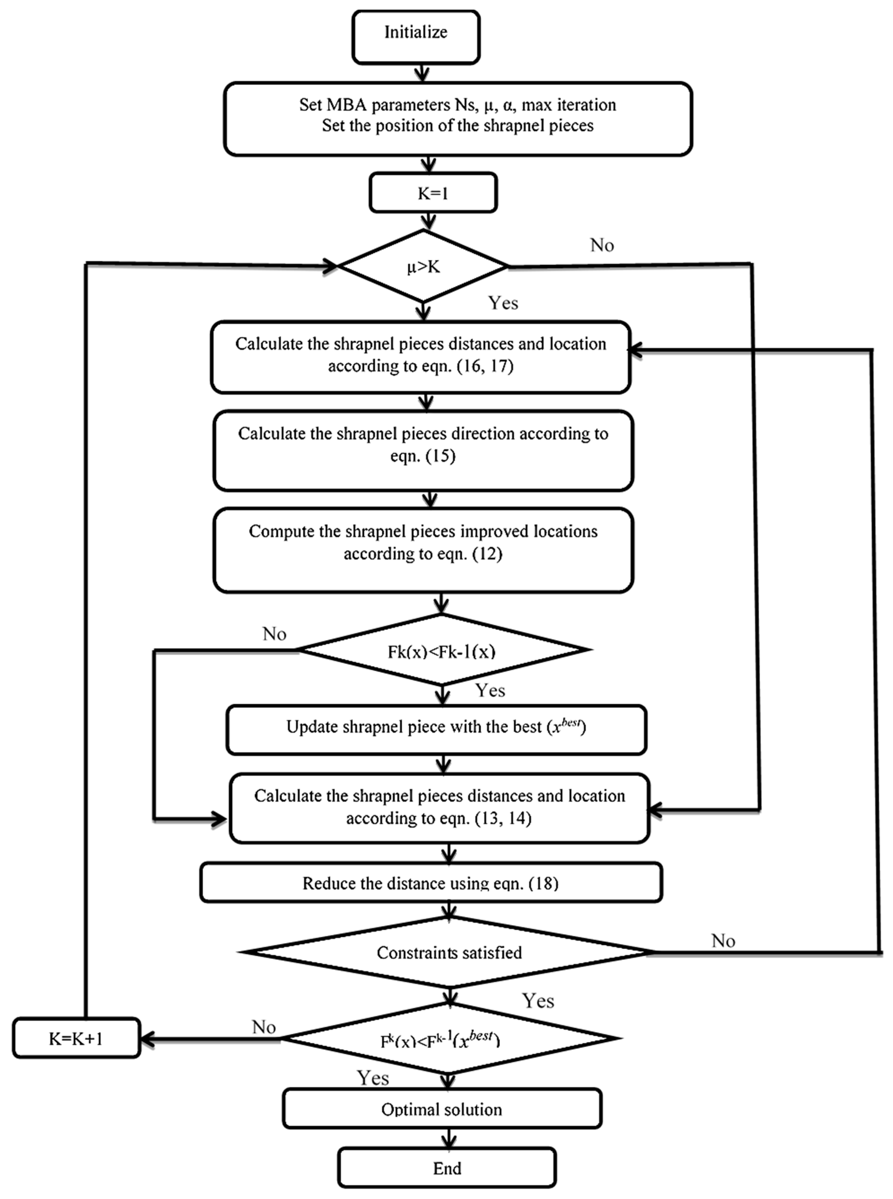
The mine blast algorithm (MBA) is a population-based algorithm, and it was first introduced in [44,45,46] as an offline algorithm. MBA was proposed and designed to solve complex control tasks. It is used in [44,46] to solve truss structure problems; results clearly illustrated the effectiveness of the method for solving problems of many design parameters and criteria. In addition, it has a fast rate of convergence to reach the optimal (best) solution and also has low burden (function computational evaluations), verifying MBA’s potential to solve complicated problems compared to other systems such as genetic algorithm and PSO. In [45], a comparative study showed that MBA was more effective than other recognized optimization algorithms in terms of computational effort and function value for sixteen engineering problems. It was applied in [47] to obtain the optimal sizing for photovoltaic (PV) fuel cells and wind turbines to supply a certain load; MBA saved 24.82%, 11.5576%, and 8.95% in the yearly cost compared with PSO, BCO, and cuckoo search algorithm, respectively. MBA was used to find the best design networks [48] of water distribution systems for minimizing the network construction costs. The cost was 5% lower (reduced from €2.17 to €2.064 million) than a conventional system. It has also been used to obtain the maximum power point of partially shaded photovoltaic systems [49], and results showed that the MBA tracker was more reliable and efficient compared to adaptive neuro-fuzzy, fuzzy logic, and PSO-based systems. In [50], optimal gain scheduling of the voltage source converters in high-voltage direct current systems was obtained to ensure the desired dynamic behavior and stability improvement. Load frequency control was designed based on a PID controller tuned by MBA for multi-interconnected areas [51], the system was robust compared to antlion, artificial bee colony, hybrid differential evolution PSO, and hybrid PSO pattern search optimizers [52]. MBA was applied to a variable-speed wind generator to evaluate the optimal parameters of the rotor current PI controller for setting rotor current close to the desired reference one and tracking the reference system frequency. Based on the above discussion, it can be said that MBA is a simple robust technique that converges quickly and requires few design control parameters.

This paper is subdivided as follows. The system model is discussed and given in Section 2. In Section 3 the design of the controller with an objective fitness function is provided. The MBA algorithm is detailed in Section 4. Results and discussion are explained in Section 5, and the conclusions are discussed in Section 6.

2. System Modeling

2.1. Basic Wind–Diesel System

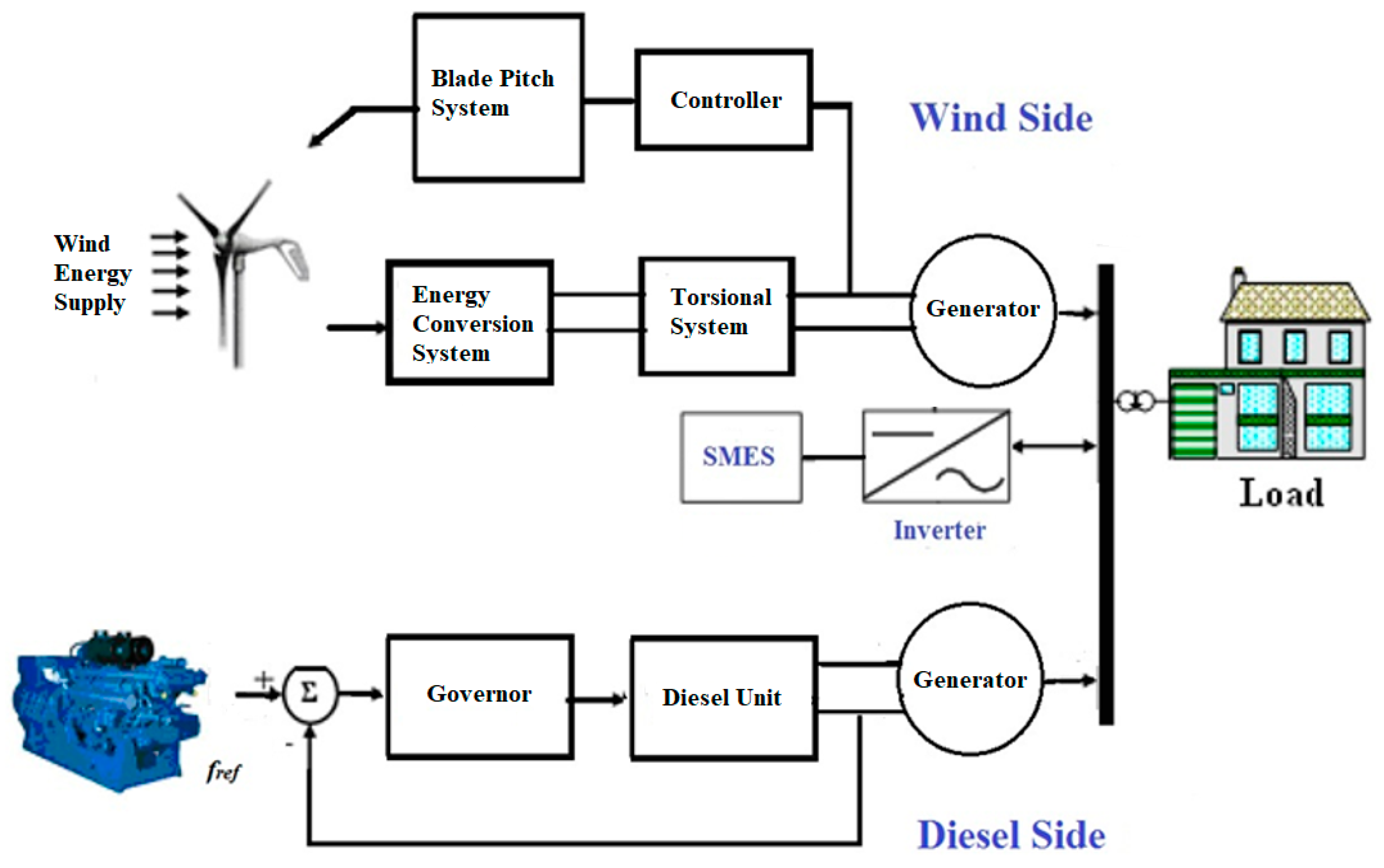
The basic diagram of the hybrid wind–diesel system [31,53,54] is shown in Figure 1. The system consists of a 200 kW diesel generator controlled by a speed governor system and a 150 kW wind turbine generator controlled by a blade pitch controller. The diesel generator, wind generator, and power system parameters under study are listed [31,53,54] in Appendix A in

Table A1. Wind, diesel, and SMES data.

Wind generator rating	150 kW
Diesel generators rating	200 kW
Load demand power	350 kW
Inertia constant of wind system, $H_w$	3.5 s
Inertia constant of diesel system, $H_d$	8.5 s
Fluid coupling of the hybrid wind and diesel system, $K_{fc}$	16.2 pu kW/Hz
Governor gain, $K_d$	16.5 pu kW/Hz
Governor time constant $T_1$	0.025 s
The hydraulic pitch actuator gain $K_{p2}$	1.25
The time constant of hydraulic pitch actuator $T_{p1}$	0.6 s
The time constant of pitch actuator $T_{p2}$	0.041 s
Gain of data fit pitch response, $K_{p3}$	1.4
Blade pitch characteristic gain, $K_{pc}$	0.08 pu kW/deg
SMES time constant $T_{sm}$	0.03 s

. The wind turbine and diesel generators’ transfer functions and model are completely illustrated in [31,53,54].

The inertia of the diesel generators and load are lumped together. The diesel governor and throttle compare the system speed (frequency) to a reference speed and compensate for speed error by changing the fuel rate.

2.2. Blade Pitch System

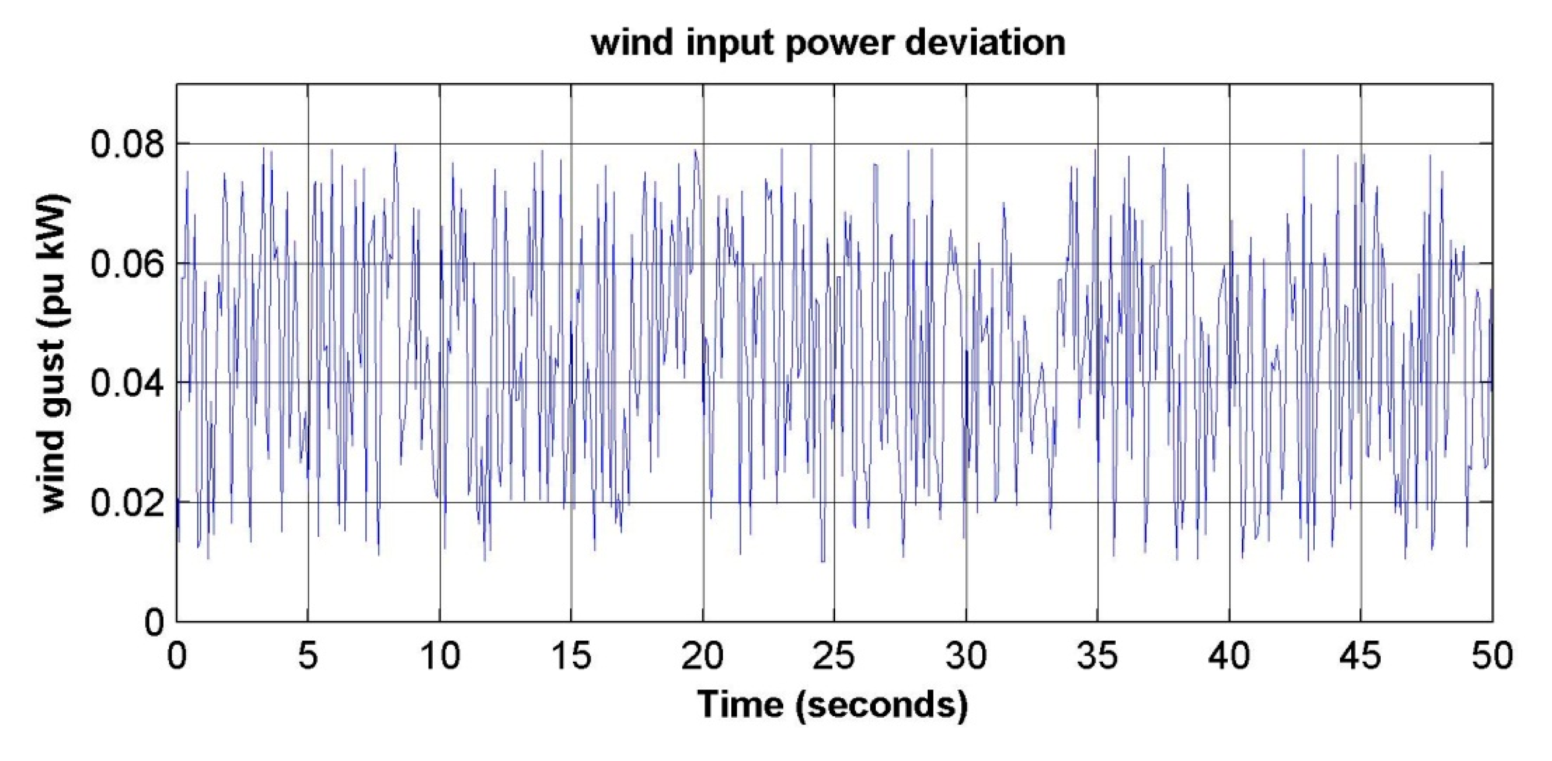
As mentioned in [55], pitch occurs when there is a variation of the wind speed. Thus, pitch angle control of the blades is a must for ensuring the continuity of energy production by reducing the turbine output power to its nominal level (power control) and protecting the turbine devices from extra high power (safety constraints) during high wind speed. In real systems, this control is basically based on using an anemometer on the nacelle to measure the wind speed and its direction. In the proposed study, the anemometer is simulated by an input variation in wind input power [53], as any variation in the wind speed will be reflected into a variation in the turbine input power ($\Delta P_w$).

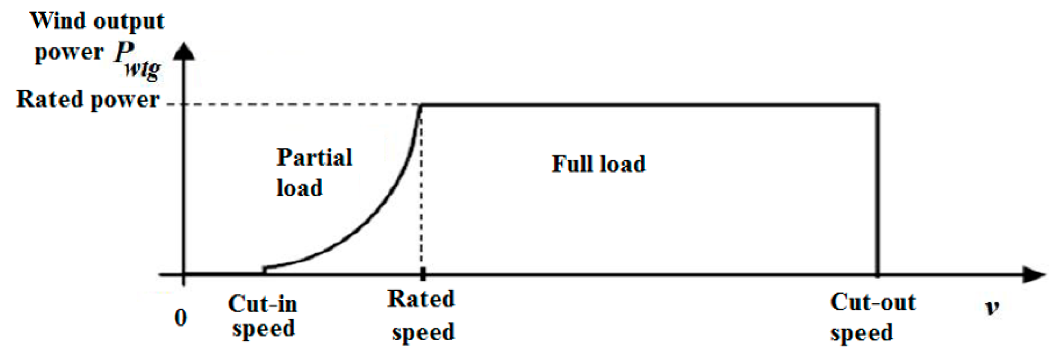
The blade angle of the wind turbine is controlled by the microprocessor-based controller. Pitch angle can be controlled according to power speed curve shown in Figure 2. The pitch control system can be illustrated by subdividing the power speed curve into four regions [29]:

(1) Below cut-in speed

When the wind speed is less than the cut in speed (3–3.5 m/s according to the wind turbine design), the value of the pitch angle must be increased to the maximum value, as the turbine output power is the smallest at this point. $P_{wtg}$ = 0 kW, so the pitch angle is fixed at 90° as the turbine output is the smallest.

(2) From cut-in to speed at which rated power occurs (partial load region)

When the wind speed is between cut in and the speed at which rated power can be obtained, the value of the pitch angle must be set at value at which the maximum power can be captured from the wind. The range of $P_{wtg}$ is from 0 to 150 kW, so the pitch angle is fixed at 10°, as energy is largest at this angle.

(3) From speed at which the rated power is captured to cut-out

When the wind speed is higher than the rated speed, the power is higher than the nominal value, so the value of the pitch angle must be increased to reduce the turbine output power. Thus, the rated electric power can still be produced. $P_{wtg}$ = 150 kW, so the pitch angle is varied from 10° to 90°.

(4) Above cut-out speed

When the wind speed is higher than its cut-out value, the value of the pitch angle must be increased to disconnect the wind turbine and set the output power to zero. $P_{wtg}$ = 0 kW, so the pitch angle is fixed at 90° for safety.

The pitch system consists of a hydraulic pitch actuator for changing the angle of the blades, a PID controller that is altered by the error signal between the power set point ($P_{\max }$) and the actual power $P_{wtg}$. It can be modeled as in [31,53,54]. The power reference set point ($P_{\max }$) can be controlled and adjusted from 25 to 150 kW. When wind turbine $P_{wtg}$ provides less power than the reference power, there will be an error difference which alters the hydraulic actuator system. Then, pitch angle control becomes active and compares the generated power to $P_{\max }$ (the power set point) and compensates for power error by changing the blade angle and thus the mechanical power; this error sets the blades’ angle to 10° (fully feathered position at shutdown). When the power output exceeds $P_{\max }$, the pitch control will be active to control for constant $P_{\max }$ power output. The specified transfer function programmed in the microprocessor controller contains a proportional–integral coefficient–differential controller.

2.3. Superconducting Magnetic Energy Storage (SMES) System

The SMES system can be modeled by a first-order function [56] with a time constant $T_{sm}$ = 0.03 s. The controller was designed as first-order compensator with a single feedback input signal, diesel frequency deviation, $\Delta f_d$.

The system block diagram is illustrated in Figure 3 [31,53,54].

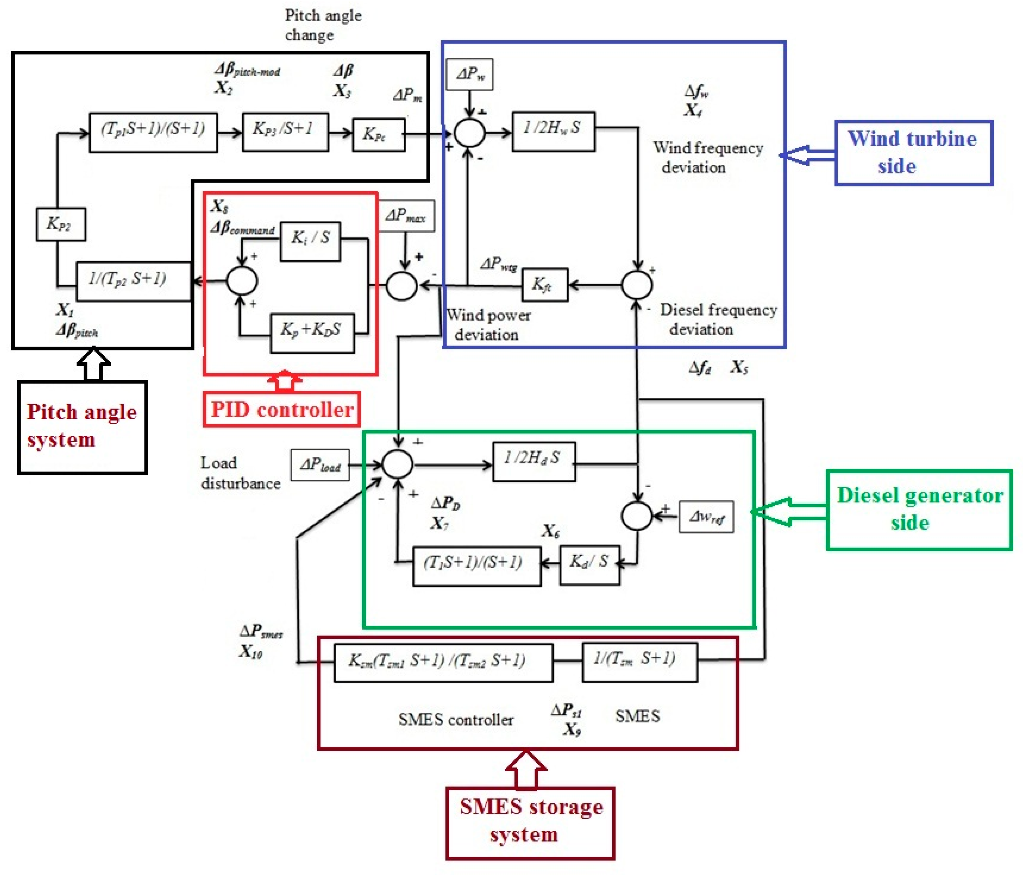
The wind–diesel dynamic behavior is modeled by the set of differential equations represented in state space as follows:

$$X^{•}=AX+BU,$$

(1)

$$Y=CX+DU,$$

(2)

where $X$ is the system state variables, it is a vector of tenth order whose elements are illustrated in Figure 3. $U$ is the system control input. $Y$ is the system output vector. A, B, C, and D are the coefficient matrices of the hybrid system.

$$U=[\Delta P_w\hspace{1em}\Delta P_{load}],$$

(3)

$$Y^{}=[\Delta f_w\hspace{1em}\Delta f_d\hspace{1em}\Delta P_d\hspace{1em}\Delta P_{wtg}\hspace{1em}\Delta P_{smes}],$$

(4)

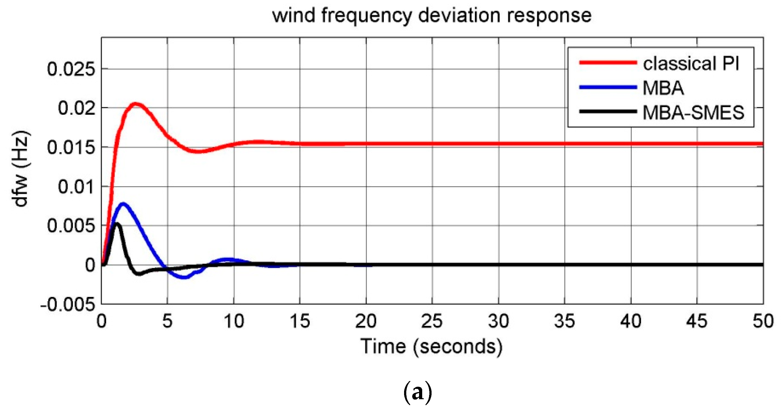
where $\Delta P_w$ and $\Delta P_{load}$ are the changes in wind and load power;

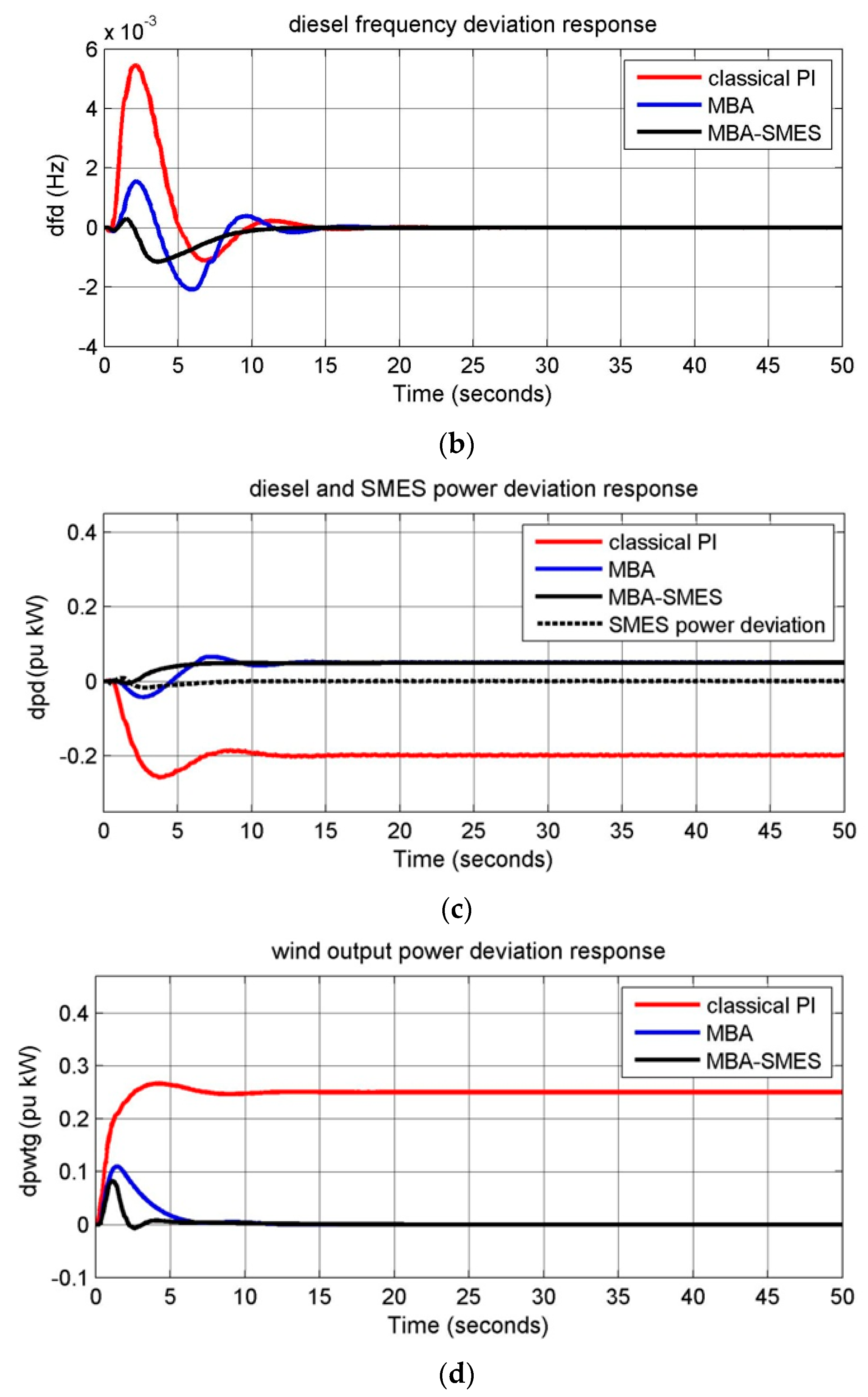
$\Delta f_w$ and $\Delta f_d$ are the change in wind and diesel frequency;

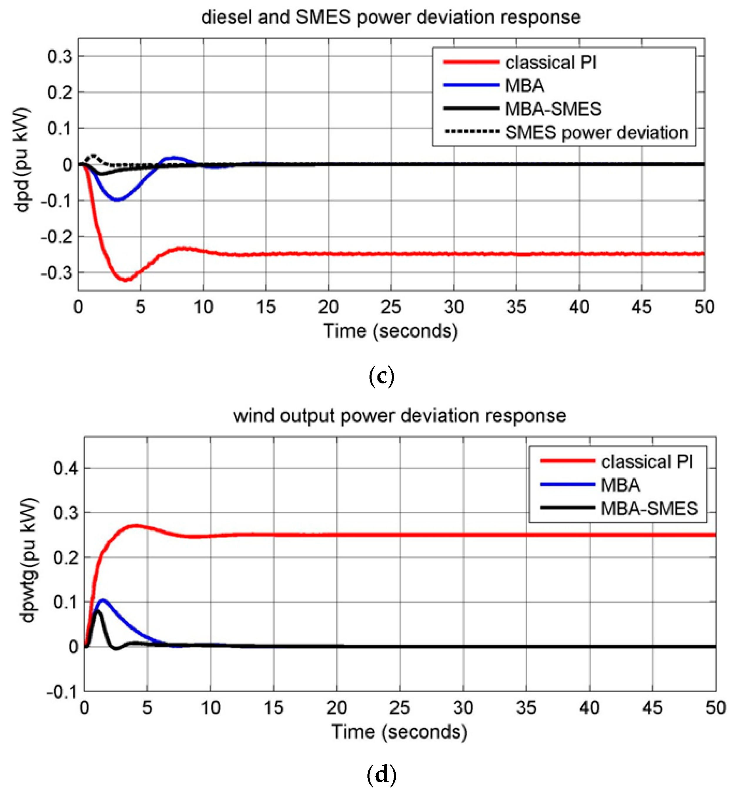
$\Delta P_d$ is the deviation in diesel power;

$\Delta P_{wtg}$ is the deviation in wind power; and

$\Delta P_{smes}$ is the deviation in SMES power.

3. Control System and Objective Fitness Function

At present, PID controllers are one of the most used industrial controllers, due to their robustness and simplicity to be understood. These systems can be designed in various structures (e.g., PID and PI) to control the wind turbine pitch angle for achieving superior dynamic performance of the wind–diesel system. In this paper, a PID controller was selected for controlling the pitch angle. The control input to the pitch actuator is formed as:

$$U_1(t)=K_p.ACE(t)+K_I{\displaystyle \underset{0}{\overset{t}{\int }}ACE{(t)}_{}}dt+K_D\frac{dACE(t)}{dt},$$

(5)

where ACE is the area control error, and $ACE(t)=(\Delta P_{\max }-\Delta P_{wtg})$.

$K_p$, $K_I$, and $K_D$ are the proportional, integral, and derivative gains. If the turbine power $P_{wtg}$ = $P_{\max }$, then $\Delta P_{\max }$ = 0. As the reference speed $w_{ref}$ is constant for the diesel generator, then the reference speed change $\Delta w_{ref}$ = 0. The system parameters including gains and time constants are listed in Appendix A. The objective function is formulated in the algorithm based on the required constraints and specifications. The performance index is the integral of absolute error (IAE) and it is used as a fitness function to find the optimal values for controllers. Thus, the objective fitness function can be rewritten as:

$$J_1={\displaystyle \underset{0}{\overset{t}{\int }}(\left|\Delta P_{wtg}\right|+\left|\Delta f_w\right|)}dt.$$

(6)

Based on Equation (6), the problem is formulated as:

Minimize $J_1$, subject to,

$$\begin{array}{l}{K}_p{}^{\min }\le K_p\le K_p{}^{\max }\\ K_I{}^{\min }\le K_I\le K_I{}^{\max }\\ K_D{}^{\min }\le K_D\le K_D{}^{\max }\end{array}$$

(7)

The range selected in the algorithm for $K_p$, $K_I$, and $K_D$ is from 0 to 120.

Also, the MBA system is used to minimize the SMES controller based on the following objective function:

$$J_2={\displaystyle \underset{0}{\overset{t}{\int }}(\left|\Delta P_D\right|+\left|\Delta f_d\right|)}dt,$$

(8)

subject to:

$$\begin{array}{l}{K}_{sm}{}^{\min }\le K_{sm}\le K_{sm}{}^{\max }\\ T_{sm1}{}^{\min }\le T_{sm1}\le T_{sm1}{}^{\max }\\ T_{sm2}{}^{\min }\le T_{sm2}\le T_{sm2}{}^{\max }\end{array}$$

(9)

where the ranges of SMES gain and time constants ($K_{sm}$, $T_{sm1}$, and $T_{sm2}$) are [10–40], [0.1–2], and [0.01–0.1], respectively.

4. Mine Blast Algorithm

4.1. Algorithm Basic Concept

The main idea is based on mine explosion, where the shrapnel pieces collide with mine bombs, resulting in their explosion. Assume that the field has bombs with different explosion powers and sizes planted underground, and the aim is to find mine locations and clear them. The one that has the most explosive and dominant effect at point x * (optimal point) has the greatest fitness function. When a mine bomb explodes, the shrapnel pieces spread and the fitness f(x) of each piece is evaluated and calculated. The existence of more explosive mines is indicated by their causalities. Each shrapnel piece collides with other bombs, leading to the explosion of the remaining mines. This collision leads to finding the most explosive and dominant mine.

4.2. Proposed Method

The MBA algorithm [45] chooses the initial point(s) randomly using the upper and lower limits. The first shot point is defined by $X_0^f$. The superscript $f$ represents the first shot point ($f$ = 1, 2, 3, 4…). The initial population (N_pop) produces a number of shrapnel pieces (individuals), and then the algorithm creates $X_0$ randomly as follows:

$$X_0=lb+rand\times (ub-lb),$$

(10)

where $X_0,ub$ and $lb$ are the first shot point and gain’s upper and lower state limits, respectively, and rand is a randomly generated number.

The current location $X_1$ of a mine bomb is given by the following equation:

$$X_1=\left\{X_m\right\}\hspace{1em}m=1,2,3,...,N_d,$$

(11)

and the new location $X_{n+1}^{}$ is:

$$X_{n+1}^f=X_{e(n+1)}^f+\exp (-\sqrt{\frac{m_{n+1}^f}{d_{n+1}^f}})X_n^f,\hspace{1em}n=0,1,2,...,$$

(12)

where $X_{n+1}^f$, $d_{n+1}^f$ are the location and distance of the exploded mine bomb. $m_{n+1}^f$ is the direction of the shrapnel. The mine location $X_{e(n+1)}^f$ is given as:

$$X_{e(n+1)}^f=d_e^f\times rand\times \cos (\theta ),\hspace{1em}n=0,1,2,...,$$

(13)

where $\theta$ is the angle of shrapnel pieces, and it equals to $360/N_s$. The algorithm explores the search space in 360° in every iteration based on $\theta$ and $d_n^f$ to get the optimal solution. The distance $d_{n+1}^f$ and the direction $m_{n+1}^f$ of shrapnel pieces are given as:

$$d_{n+1}^f=\sqrt{{(X_{n+1}^f-X_n^f)}^2+{(F_{n+1}^f-F_n^f)}^2}\hspace{1em}n=0,1,2,\dots ,$$

(14)

$$m_{n+1}^f=\frac{(F_{n+1}^f-F_n^f)}{(X_{n+1}^f-X_n^f)}\hspace{1em}n=0,1,2,\dots ,$$

(15)

where ($X_n^f$) is the previous solutions and $F$ is the fitness function value for $X$. The algorithm sets the initial distance $d_0^{}$ of shrapnel as $d_0^{}=(ub-lb)$. The proposed algorithm searches within the initial distance range $LB\langle d_0^{}\langle UB$. The exploration factor ($\mu$) is introduced, and if $\mu$ is higher than $K$, the exploration process starts. The exploration equations are:

$$d_{(n+1)}^f=d_e^f\times {(\left|randn\right|)}^2\hspace{1em}n=0,1,2,...,$$

(16)

$$X_{e(n+1)}^f=d_{n+1}^f\times \cos (\theta ),\hspace{1em}n=0,1,2,....$$

(17)

Using $\mu$, the shrapnel piece distance is modified using Equation (14). The value of $\mu$ determines the process intensity. Then, the value of $\mu$ is set to a high value to search in more regions. The initial distance $d_0^f$ is reduced. This reduction allows the algorithm to obtain the optimal solution. In general, the reduction in $d_n^f$ is given as:

$$d_n^f=\frac{d_{n-1}^f}{\exp (K/\alpha )},\hspace{1em}n=0,1,2,...,$$

(18)

where $K$ and $\alpha$ are the iteration number and reduction factor. The steps of MBA are summarized [45] and its flowchart is illustrated in Figure 4.

5. Simulation Results

Three systems are designed in this paper based on the Matlab environment, and they can be defined as:

(1) Classical PI controller:

The blade pitch controller of the hybrid wind–diesel system is not tuned.

(2) MBA system:

The blade pitch controller of the hybrid wind–diesel system is tuned based on the MBA algorithm.

(3) MBA–SMES:

The blade pitch and SMES controllers of the hybrid wind–diesel–SMES system are tuned based on the MBA algorithm. The three systems were designed and compared.

Five case studies were designed and investigated. The first case was studied based on considering the input wind power disturbance only in order to show the effect of wind speed variation (simulated in the change of input wind power). The second case was studied by considering both changes in wind and load input powers, to show the effect of wind speed and load demand variations. In third case, the hybrid systems were subjected to (random wind input power) wind gust. The fourth case was done by applying harsh operating conditions including disturbances in input wind, load power, and fluid coupling parameter variation. Finally, a detailed sensitivity analysis was made based on fluid coupling change from −30% to 30% of its nominal value. These case studies are discussed to show the effectiveness and robustness of the MBA–SMES scheme. The wind, diesel, and SMES data are defined in Table A1.

5.1. Case 1

A step increase of the wind power input 25% (system base of 350 kW) was applied to the system. Figure 5 shows the frequency and power deviations for both diesel and wind generators, including the diesel frequency deviation. In the case of the classical PI controller and as shown in Figure 5a, the maximum overshoot (M.O) of wind frequency deviation was large (0.0217 Hz) and took a longer time (2.609 s), reaching steady state in approximately 15 s. This indicates that the wind pitch system and the diesel governor did not work well. Contrarily, MBA and MBA–SMES controllers have the ability to reduce frequency deviation significantly by reducing the peak overshoot and settling time of the system response. The system performance parameters are listed in

Table 1. Wind frequency deviation performance parameters. ess: steady-state error; M.O: maximum overshoot; R.T: rise time; S.T: settling time, T.O.S: time of over shoot, U.S: under shoot.

Wind Frequency Performance Parameters Under$\mathbf{\Delta }{\mathit{P}}_{\mathit{w}}$= 0.25 pu kW	Phase of Comparison	Classical System	MBA System	MBA–SMES System
	M.O (Hz)	0.02174	0.00877	0.00559
	T.O.S (s)	2.60942	2.10438	1.34680
	U.S (Hz)	1.42 × 10−2	−1.87 × 10−3	3.44 × 10−7
	R.T (s)	0.69267	0.02932	0.00551
	S.T (s)	13.923	13.657	6.217
	ess (Hz)	1.54 × 10−2	2.37 × 10−5	4.52 × 10−7

, and the MBA–SMES maximum overshoot was about 0.00559 Hz, about 0.25 of classical and 0.63 of MBA systems, reaching its peak value (T.O.S) in 1.346 s (approximately 0.5 of classical and 0.64 of MBA systems) and its rise time (R.T) was about 0.00551 s and its settling time (S.T) was 6.217 s (0.007 of classical and 0.18 of MBA systems). As shown in Figure 5a, it is clear that the MBA–SMES system steady-state error (ess) reached zero compared to the MBA system (Hz) and classical system. Figure 5b and

Table 2. Diesel frequency deviation performance parameters.

Diesel Frequency Performance Parameters Under$\mathbf{\Delta }{\mathit{P}}_{\mathit{w}}$= 0.25 pu kW	Phase of Comparison	Classical System	MBA System	MBA–SMES System
	M.O (Hz)	0.00678	0.00309	0.00113
	T.O.S (s)	1.92034	2.27596	1.56472
	U.S (Hz)	−0.00137	−0.00216	−0.00024
	R.T (s)	4.28 × 10−4	7.98 × 10−5	4.23 × 10−6
	S.T (s)	16.070	14.705	12.915
	ess (Hz)	−1.25 × 10−6	−3.31 × 10−8	−1.51 × 10−8

illustrate the diesel frequency response; the proposed system reduced the max overshoot to 0.00113 Hz (0.0035 of classical and 0.0022 of MBA systems) in 1.56472 s (0.8148 of classical and 0.6875 of MBA systems), the rise time was about 4.23 × 10⁻⁶ s (0.0988 of classical and 0.18 of MBA systems) and the settling time was 12.915 s (0.8037 of classical and 0.8783 of MBA systems).

Figure 5c shows the diesel power deviations of the three systems with the SMES power deviation of the proposed MBA–SMES system. The SMES unit responded to system disturbances in order to damp the power oscillations rapidly. The diesel power deviation’s performance parameters are listed in

Table 3. Diesel power deviation performance parameters.

Diesel Power Performance Parameters Under$\mathbf{\Delta }{\mathit{P}}_{\mathit{w}}$=0.25 pu kW	Phase of Comparison	Classical System	MBA System	MBA–SMES System
	M.O (Hz)	0.32209	0.09848	0.02663
	T.O.S (s)	3.76956	3.12945	1.84922
	U.S (Hz)	−0.32209	−0.02663	−0.00781
	R.T (s)	1.15669	0.04055	0.00036
	S.T (s)	19.965	14.445	10.914
	ess (Hz)	−2.45 × 10−1	1.97 × 10−5	−4.41 × 10−6

. In addition, Figure 5d illustrates the wind output power deviations of the three systems. The difference of output power reference of wind turbine was set to zero (pu kW). For the classical system, the blade pitch system set the output power deviation to 25% due to the input disturbance, and then this controller did not work well. On the other hand, the proposed system based on MBA–SMES damped the output power oscillations in a very short time and their blade pitch controller set the output power deviation to zero (pu kW) by setting the M.O to 0.07923 Hz (0.0827 of classical and 0.2704 of MBA systems) and the S.T to 6.412 s (0.4993 of classical and 0.558 of MBA systems). MBA with the SMES unit enhanced the performance of the system as listed in

Table 4. Wind output power deviation performance parameters.

Wind Power Parameters Under$\mathbf{\Delta }{\mathit{P}}_{\mathit{w}}$= 0.25 pu kW	Phase of Comparison	Classical System	MBA System	MBA–SMES System
	M.O (Hz)	0.27048	0.10383	0.07923
	T.O.S (s)	3.98293	1.49359	1.06685
	U.S (Hz)	2.27 × 10−1	−4.41 × 10−3	−5.51 × 10−5
	R.T (s)	1.51862	0.00113	0.00088
	S.T (s)	12.842	11.491	6.412
	ess (Hz)	2.50 × 10−1	1.75 × 10−6	1.37 × 10−6

.

5.2. Case 2

The proposed system was tested to confirm its effectiveness. The operating conditions were represented as 5% change in load power with 25% change in wind input power. Results are presented in Figure 6 showing the system dynamic response of the three control schemes including the wind frequency, diesel frequency, diesel output power, and wind output power. From Figure 6a and

Table 5. Wind frequency deviation performance parameters.

Wind Frequency Performance Parameters Under$\mathbf{\Delta }{\mathit{P}}_{\mathit{w}}$= 0.25 pu kW$\mathbf{\Delta }{\mathit{P}}_{\mathit{l}\mathit{o}\mathit{a}\mathit{d}}$= 0.05 pu kW	Phase of Comparison	Classical System	MBA System	MBA–SMES System
	M.O (Hz)	0.02050	0.00775	0.00525
	T.O.S (s)	2.5641	1.6382	1.1396
	U.S (Hz)	0.01422	−0.00163	−0.00119
	R.T (s)	0.75442	0.00048	0.00032
	S.T (s)	9.407	11.271	7.914
	ess (Hz)	1.54e-02	4.63 × 10−8	1.51 × 10−8

, the wind frequency deviation response was clearly enhanced by decreasing M.O to 0.00525 Hz (0.25 times of classical and 0.67 of MBA systems), R.T to 0.00032 s (4.21 × 10⁻⁴ of classical and 0.6545 MBA systems), and S.T to 7.91445 s (0.8413 of classical and 0.7022 MBA systems).

More illustrative results can be obtained from Figure 5b to Figure 6d and in the tables below (

Table 6. Diesel frequency deviation performance parameters.

Diesel Frequency Performance Parameters Under$\mathbf{\Delta }{\mathit{P}}_{\mathit{w}}$= 0.25 pu kW$\mathbf{\Delta }{\mathit{P}}_{\mathit{l}\mathit{o}\mathit{a}\mathit{d}}$= 0.05 pu kW	Phase of Comparison	Classical System	MBA System	MBA–SMES System
	M.O (Hz)	5.13675	4.91168	3.63247
	T.O.S (s)	−0.00110	−0.00208	−0.00115
	U.S (Hz)	0.02637	0.03174	0.00011
	R.T (s)	13.004	14.561	12.436
	S.T (s)	2.1367	5.91168	3.63247
	ess (Hz)	−1.09 × 10−6	−2.49 × 10−7	7.54 × 10−8

,

Table 7. Diesel power deviation performance parameters.

Diesel Power Performance Parameters Under$\mathbf{\Delta }{\mathit{P}}_{\mathit{w}}$= 0.25 pu kW$\mathbf{\Delta }{\mathit{P}}_{\mathit{l}\mathit{o}\mathit{a}\mathit{d}}$= 0.05 pu kW	Phase of Comparison	Classical System	MBA System	MBA–SMES System
	M.O (Hz)	0.2576375	0.0652	0.05002
	T.O.S (s)	3.7749287	6.98005	4.8575
	U.S (Hz)	−0.2576375	0.04244	0.04516
	R.T (s)	1.2329223	1.31724	3.61641
	S.T (s)	10.894785	12.3499	9.3131
	ess (Hz)	−0.199296	0.050165	0.050001

and

Table 8. Wind output power deviation performance parameters.

Wind Power Performance Under$\mathbf{\Delta }{\mathit{P}}_{\mathit{w}}$= 0.25 pu kW$\mathbf{\Delta }{\mathit{P}}_{\mathit{l}\mathit{o}\mathit{a}\mathit{d}}$= 0.05 pu kW	Phase of Comparison	Classical System	MBA System	MBA–SMES System
	M.O (Hz)	0.26646	0.10946	0.08300
	T.O.S (s)	4.20227	1.42450	1.13960
	U.S (Hz)	2.28 × 10−1	−7.84 × 10−6	−6.39 × 10−3
	R.T (s)	1.51 × 101	2.86 × 10−3	2.09 × 10−5
	S.T (s)	12.828	11.205	6.456
	ess (Hz)	2.50 × 10−1	4.79 × 10−6	−9.76 × 10−7

). As in Figure 6c, the MBA–SMES system set the output power deviation to 0.05 pu kW with M.O to 3.63247 Hz (0.67 of MBA system). Moreover, Figure 6d illustrates the wind power deviations of all systems. The difference of turbine output power reference was set to zero (pu kW). The proposed system based on MBA–SMES damped the output power oscillations and the blade pitch controller set the output power deviation to zero (pu kW) by setting the M.O to 0.083005 Hz (0.1 of MBA systems) and the S.T to 6.455 s (0.576 of MBA systems).

This improvement was because the SMES system discharged its power in a very short time, as can be seen in Figure 6c. This action aided the main system in withstanding the disturbances in load and wind power. In addition, the steady-state error reached zero.

5.3. Case 3

The studied systems were subjected to wind gust (random wind input power) as seen in Figure 7. As mentioned previously, using an anemometer is necessary to measure the wind speed and its direction. In this study, the input change in wind speed measured by the anemometer was simulated by variation in the wind input power, as any variation in the wind speed will be reflected into a variation in the turbine input power ($\Delta P_w$). The simulation results in Figure 8 show that the MBA–SMES system was better than that of the classical and MBA systems. As illustrated in Figure 8a, the wind frequency deviation of the MBA–SMES system oscillated between −0.4 × 10⁻³ and 0.4 × 10⁻³ Hz around zero, while the MBA system oscillates between −1.2 × 10⁻³ and 1.1 × 10⁻³ Hz around zero and the classical system oscillated between −2.5 × 10⁻³ and 4.5 × 10⁻³ Hz around 2.5 × 10⁻³ Hz. The MBA–SMES system gave the better response for the frequency and power deviation responses compared to other systems. This also can be seen in the remaining figures (Figure 8b–d).

5.4. Case 4

The systems were tested under harsh conditions to confirm their effectiveness. The operating conditions were represented as 5% change in load power with 25% change in input wind power and 25% decrease in $K_{fc}$. $K_{fc}$ was selected because it is the dominant parameter in the hybrid system [20]. Results are presented in Figure 9a–d and show that the system dynamic response of the proposed MBA-based control scheme could withstand these severe operating conditions. It can be verified from

Table 9. Wind frequency deviation performance parameters.

System Frequency Performance parameters Under$\mathbf{\Delta }{\mathit{P}}_{\mathit{w}}$= 0.25 pu kW$\mathbf{\Delta }{\mathit{P}}_{\mathit{l}\mathit{o}\mathit{a}\mathit{d}}$= 0.05 pu kW$K_{fc}$= 1.25$K_{fc}$	Phase of Comparison	Classical System	MBA System	MBA–SMES System
	M.O (Hz)	0.01768	0.00653	0.00451
	T.O.S (s)	2.38784	1.59189	1.08538
	U.S (Hz)	0.01122	−0.00165	−0.00094
	R.T (s)	6.79 × 10−1	9.95 × 10−4	2.53 × 10−5
	S.T (s)	9.4343	12.6615	8.5455
	ess (Hz)	1.23 × 10−2	4.68 × 10−8	−1.27 × 10−7

that the MBA–SMES system decreased the maximum overshoot to 0.0045 Hz (0.2549 of classical and 0.689 of MBA based systems) and the settling time to 8.54552 s. The simulation results prove the robustness and effectiveness of the proposed MBA–SMES-based controller over MBA and PI classical systems.

5.5. Case 5

In this case, systems were tested under parameter variation conditions to confirm their effectiveness. The fluid coupling coefficient was selected as mentioned above (the control system response is sensitive to this parameter). The operating conditions were represented as 5% change in load power, 25% change in wind input power, and a variation in $K_{fc}$ from −30% to 30%. The performance index used was the IAE. Results are presented in Figure 10 and Figure 11 and show the system dynamic response of the systems. As the fluid coupling decreased, the IAE values of the classical PI system increased sharply. However, the values of the proposed MBA–SMES scheme were much lower, and almost constant.

Table 10. System frequency performance parameters under fluid coupling variation.

		Wind and Diesel Frequencies
		$\mathbf{\Delta }{\mathit{f}}_{\mathit{w}}$				$\mathbf{\Delta }{\mathit{f}}_{\mathit{d}}$
		M.O (Hz)	R.T (s)	S.T (s)	ess (Hz)	M.O (Hz)	R.T (s)	S.T (s)	ess (Hz)
$K_{fc}$	−30	0.0069	2.59 × 10−5	7.406	−2.10 × 10−7	0.0012	0.00096	12.239	4.95 × 10−7
	−15	0.0059	2.81 × 10−6	7.419	−1.87 × 10−8	0.0012	0.00016	12.335	2.24 × 10−7
	0	0.0053	3.18 × 10−4	7.914	1.52 × 10−8	0.0012	0.00011	12.436	7.55 × 10−8
	15	0.0048	1.79 × 10−6	8.406	−1.16 × 10−8	0.0012	0.00033	12.471	2.39 × 10−7
	30	0.0044	2.76 × 10−5	8.473	−1.33 × 10−7	0.0012	0.00055	12.283	5.16 × 10−7

shows the MBA–SMES system’s response under fluid coupling variation. At the change in $K_{fc}$ equal to −30% and 30%, the steady state error change was 1.25%. For rise time, the change from base case (no fluid coupling change) did not exceed 0.5%. The settling time change did not exceed 5%. From the discussion it can be observed that all performance parameters varied within acceptable limits and were approximately equal to the obtained values with the nominal system. So, the MBA–SMES based system was robust for fluid coupling variation and effective compared to other systems.

6. Conclusions

A robust MBA-based control scheme of the isolated hybrid wind–diesel system was designed in this paper to tune the gains of two controllers. The first were the PID gains of the blade pitch controller and the second were those of the SMES controller. The MBA–SMES system was compared with the classical PI- and MBA-based controllers. Five case studies were considered in the simulation under load and input wind power disturbances and harsh conditions with parameter variation for the fluid coupling of the wind and diesel generators. The simulation results confirmed the effectiveness and robustness of the proposed MBA–SMES system compared with other systems. The main improvements can be summarized in the following points.

• The proposed MBA–SMES system was able to damp the output deviation in frequencies and power of the system, reducing overshoot and settling time. For wind frequency, the MBA–SMES maximum overshoot was reduced to 0.00559 Hz (0.25 of classical system), it reached its peak value in 1.346 s (approximately 0.5 of classical), the rise time was about 0.00551 s (0.008 of classical system), meaning that the reduction percent reached 75% of the classical system. Its settling time was 6.2166 s (0.4465 of classical system).
• The main improvements were due to the existence of SMES system, which aided the main system in responding to the disturbances. For wind frequency, MBA–SMES reduced overshoot to 0.00637 Hz (0.63 of MBA system) in 1.346 s (0.64 of MBA system). This means that the reduction percent reached 36% that of the MBA system, the rise time was 0.00551 s (0.19 of MBA system), and the settling time was 6.2166 s (0.18 of MBA system).
• The MBA–SMES based system was robust to fluid coupling variation and was effective compared to other systems. At the change in $K_{fc}$ ranging from −30% to 30%, the steady state error change was 1.25%. For rise time, the change from base case did not exceed 0.5%. The settling time change did not exceed 5%. Values of the performance parameters varied within acceptable limits, and were near the obtained values with the nominal system parameters.
• The MBA optimization algorithm was a very robust technique; it had better selectivity than the gains of PID blade pitch and SMES controllers. Also, this algorithm is simple and converged quickly during the optimization process.

It is recommended to use MBA after modification for solving multi-objective optimization systems to optimize the hybrid system under multi-objective functions such as the mechanical stress on the wind turbine blades. In addition, wind–diesel control systems can be combined with photovoltaic systems, battery storage, fuel cells, etc., enlarging the scale of hybrid systems from small-scale (micro-grid of 350 kW capacities) to medium- and large-scale power systems.

References

1. Hunter, R.; Elliot, G. Wind-Diesel Systems. A Guide to Technology and Its Implementation; University Press: Cambridge, UK, 1994. [Google Scholar]
2. Senjyu, T.; Omine, E.; Hayashi, D.; Sekine, H.; Funabashi, T. Application of decentralized control for remote power system stabilization by installing renewable energy power plant. IEEJ Trans. Electr. Electron. Eng. 2008, 3, 473–481. [Google Scholar] [CrossRef]
3. Khelif, A.; Talha, A.; Belhamel, M.; Arab, A.H. Feasibility study of hybrid Diesel-PV power plants in the southern of Algeria: Case study on AFRA power plant. Int. J. Electr. Power Energy Syst. 2013, 43, 553–564. [Google Scholar] [CrossRef]
4. Kassem, A.M.; Yousef, A.M. Robust control of an isolated hybrid wind-diesel power system using Linear Quadratic Gaussian approach. Int. J. Electr. Power Energy Syst. 2011, 33, 1092–1100. [Google Scholar] [CrossRef]
5. Hu, Y.; Morales, J.M.; Pineda, S.; Sánchez, M.J.; Solana, P. Dynamic multi-stage dispatch of isolated wind diesel power systems. Energy Convers. Manag. 2015, 103, 605–615. [Google Scholar] [CrossRef]
6. Bernal-Agustín, J.L.; Dufo-Lopez, R. Simulation and optimization of stand-alone hybrid renewable energy systems. Renew. Sustain. Energy Rev. 2009, 13, 2111–2118. [Google Scholar] [CrossRef]
7. Lipman, N.H. Overview of wind/diesel systems. Renew. Energy 1994, 5, 595–617. [Google Scholar] [CrossRef]
8. Das, D.; Roy, A.; Sinha, N. GA Based Frequency Controller for Solar Thermal-Diesel-Wind Hybrid Energy Generation/Energy Storage System. Int. J. Electr. Power Energy Syst. 2012, 43, 262–279. [Google Scholar] [CrossRef]
9. Sebastian, R.; Alzola, R. Simulation of an Isolated Wind Diesel System with Battery Energy Storage. Int. J. Electr. Power Syst. Res. 2011, 81, 677–686. [Google Scholar] [CrossRef]
10. Tripathy, S.C.; Kalantar, M.; Balasubramanian, R. Dynamics and stability of a hybrid wind-diesel power system. Energy Convers. Manag. 1992, 33, 1063–1072. [Google Scholar] [CrossRef]
11. Tripathy, S.C.; Kalantar, M.; Balasubramanian, R. Stability simulation and parameter optimization of a hybrid wind-diesel power generation system. Int. J. Energy Res. 1992, 16, 31–42. [Google Scholar] [CrossRef]
12. Bhatti, T.S.; Bansal, N.K. Load frequency control of isolated wind diesel hybrid power systems. Energy Convers. Manag. 1997, 38, 829–837. [Google Scholar] [CrossRef]
13. Bhatti, T.S.; Al-Ademi, A.A.F.; Bansal, N.K. Dynamics and control of isolated wind-diesel power systems. Int. J. Energy Res. 1995, 19, 729–740. [Google Scholar] [CrossRef]
14. Supriyadi, C.; Nandar, A. Parameter Optimization of Pitch Controller for Robust Frequency Control in an Isolated Wind-diesel Hybrid Power System Using Genetic Algorithm. TELKOMNIKA 2008, 6, 145–154. [Google Scholar]
15. Lotfy, M.; Senjyu, T.; Farahat, M.; Abdel-Gawad, A.; Yona, A. A Frequency Control Approach for Hybrid Power System Using Multi-Objective Optimization. Energies 2017, 10, 80. [Google Scholar] [CrossRef]
16. Supriyadi, A.N.C.; Takano, H.; Murata, J.; Goda, T.; Hashiguchi, T. Adaptive frequency control for hybrid wind-diesel power system using system estimator. In Proceedings of the IEEE International Conference on Power System Technology (POWERCON), Auckland, New Zealand, 30 October–2 November 2012; pp. 1–6. [Google Scholar]
17. Supriyadi, A.; Nandar, A. Robust PI control of smart controllable load for frequency stabilization of microgrid power system. Renew. Energy 2013, 56, 16–23. [Google Scholar]
18. Tarkeshwar, M.; Mukherjee, V. A novel quasi-oppositional harmony search algorithm and fuzzy logic controller for frequency stabilization of an isolated hybrid power system. Int. J. Electr. Power Energy Syst. 2015, 66, 247–276. [Google Scholar] [CrossRef]
19. Lasheen, A.; Elshafei, A. Wind-turbine collective-pitch control via fuzzy predictive algorithm. Renew. Energy 2016, 87, 298–306. [Google Scholar] [CrossRef]
20. Viveiros, C.; Melício, R.; Igreja, J.; Mendes, V.M.F. Performance assessment of a wind energy conversion system using a hierarchical controller structure. Energy Convers. Manag. 2015, 93, 40–48. [Google Scholar] [CrossRef]
21. Dahbi, A.; Nait-Said, N.; Nait-Said, M.S. A novel combined MPPT pitch angle control for wide range variable speed wind turbine based on neural network. Int. J. Hydrogen Energy 2015, 41, 9427–9442. [Google Scholar] [CrossRef]
22. Kumari, N.; Jha, A.N. Frequency Response Enhancement of Hybrid Power System by Using PI Controller Tuned with PSO Technique. Int. J. Adv. Comput. Res. 2014, 4, 116–122. [Google Scholar]
23. Ali, R.; Mohamed, T.; Qudaih, Y.; Mitani, Y. A New Load Frequency Control Approach in an Isolated Small Power Systems Using Coefficient Diagram Method. Int. J. Electr. Power Energy Syst. 2014, 56, 110–116. [Google Scholar] [CrossRef]
24. Borhanazad, H.; Mekhilef, S.; Ganapathy, V.G.; Delshad, M.M.; Mirtaheri, A. Optimization of micro-grid system using MOPSO. Renew. Energy 2014, 71, 295–306. [Google Scholar] [CrossRef]
25. Behera, S.; Subudhi, B.; Pati, B.B. Design of PI controller in pitch control of wind turbine: A comparison of PSO and PS algorithm. Int. J. Renew. Energy Res. 2016, 6, 271–281. [Google Scholar]
26. Farag, K.; Abo-Elyousr, F.K.; Elnozahy, A.A. Bi-objective economic feasibility of hybrid micro-grid systems with multiple fuel options for islanded areas in Egypt. Renew. Energy 2018, 128, 37–56. [Google Scholar]
27. Chaiyatham, T.; Ngamroo, I.; Pothiya, S.; Vachirasricirikul, S. Design of Optimal Fuzzy Logic-PID Controller Using Bee Colony Optimization for Frequency Control in an Isolated Wind-Diesel System. In Proceedings of the Transmission and Distribution Conference and Exposition: Asia and Pacific, Seoul, Korea, 26–30 October 2009. [Google Scholar]
28. Mishra, S.; Mallesham, G.; Jha, A. Design of Controller and Communication for Frequency Regulation of a Smart Microgrid. IET Renew. Power Gener. 2012, 6, 6248–6258. [Google Scholar] [CrossRef]
29. Howlader, A.M.; Izumi, Y.; Uehara, A.; Urasaki, N.; Senjyu, T.; Saber, A. A robust H controller based frequency control approach using the wind battery coordination strategy in a small power system. Int. J. Electr. Power Energy Syst. 2014, 58, 190–198. [Google Scholar] [CrossRef]
30. Muhando, B.E.; Wies, R.W. Nonlinear H constrained feedback control for grid-interactive WECS under high stochasticity. IEEE Trans. Energy Convers. 2011, 26, 1000–1009. [Google Scholar] [CrossRef]
31. Barisal, A.K.; Nayak, S.K. Load frequency control of wind diesel hybrid power system using DE algorithm. In Proceedings of the 10th International Conference on Intelligent Systems and Control (ISCO), Coimbatore, India, 7–8 January 2016; pp. 1–6. [Google Scholar]
32. Ramli, M.A.M.; Bouchekara, H.R.E.H.; Alghamdi, A.S. Optimal sizing of PV/wind/diesel hybrid microgrid system using multi-objective self-adaptive differential evolution algorithm. Renew. Energy 2018, 121, 400–411. [Google Scholar] [CrossRef]
33. Khooban, M.H.; Niknam, T.; Blaabjerg, F.; Davari, P.; Dragicevic, T. A robust adaptive load frequency control for micro-grids. ISA Trans. 2016, 65, 220–229. [Google Scholar] [CrossRef]
34. Shabani, H.; Vahidi, B.; Ebrahimpour, M. A robust PID controller based on imperialist competitive algorithm for load-frequency control of power systems. ISA Trans. 2013, 52, 88–95. [Google Scholar] [CrossRef]
35. Padhan, D.G.; Majhi, S. A new control scheme for PID load frequency controller of single-area and multi-area power systems. ISA Trans. 2013, 52, 242–251. [Google Scholar] [CrossRef]
36. Zamani, A.; Barakati, S.M.; Yousofi-Darmian, S. Design of a fractional order PID controller using GBMO algorithm for load–frequency control with governor saturation consideration. ISA Trans. 2016, 64, 55–66. [Google Scholar] [CrossRef]
37. Zheng, A.; Zhou, J.; Xu, Y.; Zhang, Y.; Qian, Z. A distributed model predictive control based load frequency control scheme for multi-area interconnected power system using discrete-time Laguerre functions. ISA Trans. 2017, 68, 127–140. [Google Scholar] [CrossRef]
38. Ali, S.; Yang, G.; Huang, C. Performance optimization of linear active disturbance rejection control approach by modified bat inspired algorithm for single area load frequency control concerning high wind power penetration. ISA Trans. 2018, 81, 163–176. [Google Scholar] [CrossRef]
39. Gampa, S.R.; Das, D. Real power and frequency control of a small isolated power system. Int. J. Electr. Power Energy Syst. 2015, 64, 221–232. [Google Scholar] [CrossRef]
40. Pan, I.; Das, S. Kriging Based Surrogate Modeling for Fractional Order Control of Microgrids. IEEE Trans. Smart Grid 2015, 6, 36–44. [Google Scholar] [CrossRef]
41. Ribeiro, P.; Johnson, B.; Crow, M.; Arsoy, A.; Liu, Y. Energy Storage Systems for Advanced Power Applications. Proc. IEEE 2001, 89, 1744–1756. [Google Scholar] [CrossRef]
42. Antony, A.P.; Shaw, D.T. Empowering the electric grid: Can SMES coupled to wind turbines improve grid stability? Renew. Energy 2016, 89, 224–230. [Google Scholar] [CrossRef]
43. Schainker, R. Executive Overview: Energy Storage Options for a Sustainable Energy Future. In Proceedings of the IEEE Power Engineering Society General Meeting, Denver, CO, USA, 6–10 June 2004. [Google Scholar]
44. Sadollah, A.; Bahreininejad, A.; Eskandar, H.; Hamdi, M. Mine blast algorithm for optimization of truss structures with discrete variables. Comput. Struct. 2012, 10, 49–63. [Google Scholar] [CrossRef]
45. Sadollah, A.; Bahreininejad, A.; Eskandar, H.; Hamdi, M. Mine blast algorithm: A new population based algorithm for solving constrained engineering optimization problems. Appl. Soft Comput. 2013, 13, 2592–2612. [Google Scholar] [CrossRef]
46. Sadollah, A.; Eskandar, H.; Bahreininejada, A.; Kim, J.H. Water cycle, Mine blast and improved mine blast algorithms for discrete sizing optimization of truss structures. Comput. Struct. 2015, 149, 1–16. [Google Scholar] [CrossRef]
47. Fathy, A. A reliable methodology based on mine blast optimization algorithm for optimal sizing of hybrid PV-wind-FC system for remote area in Egypt. Renew. Energy 2016, 95, 367–380. [Google Scholar] [CrossRef]
48. Sadollah, A.; Yoo, D.G.; Kim, J.H. Improved mine blast algorithm for optimal cost design of water distribution systems. Eng. Optim. 2014, 47, 1602–1618. [Google Scholar] [CrossRef]
49. Fathy, A.; Rezk, H. A novel methodology for simulating maximum power point trackers using mine blast optimization and teaching learning based optimization algorithms for partially shaded photovoltaic system. J. Renew. Sustain. Energy 2016, 8, 023503. [Google Scholar] [CrossRef]
50. Ramadan, H.S.; Fathy, A.; Becherif, M. Optimal gain scheduling of VSC-HVDC system sliding mode control via artificial bee colony and mine blast algorithms. IET Gener. Transm. Distrib. 2018, 12, 661–669. [Google Scholar]
51. Fathy, A.; Kassem, A.M.; Abdelaziz, A.Y. Optimal design of fuzzy PID controller for deregulated LFC of multiarea power system via mine blast algorithm. Comput. Appl. 2018, 1–21. [Google Scholar] [CrossRef]
52. Fathy, A.; El-baksawi, O. PI Controller Parameters Design of Doubly Fed Induction Generator Based on Mine Blast Algorithm. In Proceedings of the IEEE International Conference on Power and Energy (PECON), Melaka City, Malaysia, 28–30 November 2016; pp. 740–745. [Google Scholar]
53. Lotfy, M.E.; Senjyu, T.; Abdel-Fattah; Farahat, M.; Abdel-Gawad, A.F.; Yona, A. Enhancement of a Small Power System Performance Using Multi-Objective Optimization. IEEE Access 2017, 5, 6212–6224. [Google Scholar] [CrossRef]
54. Das, D.; Adityaa, S.; Kothari, D. Dynamics of Diesel and Wind Turbine Generators on an Isolated Power System. International. J. Electr. Power Energy Syst. 1999, 21, 183–189. [Google Scholar] [CrossRef]
55. Abdeldjalil, D.; Nasreddine, N.S.; Mohamed-said, N.S. A novel combined MPPT-pitch angle control for wide range variable speed wind turbine based on neural network. Int. J. Hydrogen Energy 2016, 41, 9427–9442. [Google Scholar]
56. Mitani, Y.; Tsuji, K.; Murakami, Y. Application of Superconducting Magnet Energy Storage to Improve Power System Dynamic Performance. IEEE Trans. Power Syst. 1988, 3, 1418–1425. [Google Scholar] [CrossRef]
Figure 1. Basic wind–diesel–SMES (superconducting magnetic energy storage) system.
Energies 12 03110 g001
Figure 2. Output power vs. wind speed characteristic.
Energies 12 03110 g002
Figure 3. Hybrid wind–diesel block diagram system. PID: proportional–integral–differential.
Energies 12 03110 g003
Figure 4. Flow chart of the mine blast algorithm (MBA).
Energies 12 03110 g004
Figure 5. The system transient response curves for deviation in (a) wind frequency, (b) diesel frequency, (c) diesel output power, and (d) wind output power for 25% change in wind input power.
Energies 12 03110 g005aEnergies 12 03110 g005b
Figure 6. The system transient response curves for deviation in (a) wind frequency, (b) diesel frequency, (c) diesel output power, and (d) wind output power for 5% step load change and 25% change in input wind power.
Energies 12 03110 g006aEnergies 12 03110 g006b
Figure 7. Random wind input power.
Energies 12 03110 g007
Figure 8. The system transient response curves for deviation in (a) wind frequency, (b) diesel frequency, (c) diesel output power, and (d) wind output power for random input wind power.
Energies 12 03110 g008aEnergies 12 03110 g008b
Figure 9. The system transient response curves deviation in (a) wind frequency, (b) diesel frequency, (c) diesel output power, and (d) wind output power for 5% step load change with 25% change in input wind power and 25% K f c .
Energies 12 03110 g009aEnergies 12 03110 g009b
Figure 10. Integral of absolute error (IAE) for wind frequency deviation under the change in K f c .
Energies 12 03110 g010
Figure 11. IAE for diesel frequency deviation under change in K f c .
Energies 12 03110 g011