1. Introduction
The level of global CO
2 emissions associated with energy production is constantly increasing. An increase in CO
2 emissions by 1.4% was observed in 2017 compared to 2016, which is an increase of 460 million Mg, and the highest global CO
2 emissions to date amount to 32.5 billion Mg. The increase in carbon dioxide emissions associated with energy production is a serious warning and shows that global efforts carried out so far to combat climate change are insufficient and are not able to achieve the objectives of the Paris Agreement [
1]. The results of the work of the International Panel on Climate Change (IPCC) clearly show that without additional measures to reduce greenhouse gas emissions, the global average atmospheric temperatures at the earth’s surface will increase from 3.7 °C to 4.8 °C in 2100 compared to the level from before the industrial era [
2].
Scenarios where the atmospheric CO
2 concentration is approximately 450 ppm by 2100 are consistent with maintaining global temperatures below 2 °C. Such scenarios foresee a significant reduction in greenhouse gas emissions in the coming decades and require radical changes in energy systems and the systematic introduction of low-carbon technologies [
3]. The Sustainable Development Scenario developed by the International Energy Agency (IEA) sets the path to achieving long-term climate goals. In the near future, this scenario assumes a slight increase in the volume of CO
2 emissions, reaching the peak level, and then a sharp decline by 2020. Regarding the energy sector, this scenario requires an increase in the volume of energy produced from renewable sources by an average of 700 TWh per year, an increase of 80% compared to an increase of 380 TWh registered in 2017. It was estimated that the share of energy from low-emission sources must increase by 1.1% annually. In addition, this scenario assumes that carbon capture, utilization and storage (CCUS) technologies will play an important role in reducing CO
2 emissions in the industrial and energy sectors [
4]. The key factor limiting the possibility of using carbon capture and storage (CCS) technology in climate plans is the availability and recognition of appropriate geological formations and structures for underground CO
2 storage. Numerous analyses have been developed on a global, regional and local scale regarding the geological potential of CO
2 storage. Estimates of the global geological potential of CO
2 storage can vary widely, as work is ongoing to improve the calculation methodology and develop an international classification system [
5]. Several studies have suggested that there is a large global potential for efficient storage of large amounts of CO
2 in geological formations and structures, such as deep saline aquifers and depleted oil and gas fields. The estimated global CO
2 storage capacity is more than fifty times the current global CO
2 emissions, which means there is a sufficiently large potential to inject carbon dioxide into geological formations for at least the next 50 years, assuming current annual CO
2 emission levels [
3].
CO
2 has been used to support oil production (EOR) since the 1950s [
6]. Research related to the use of technologies for the capture and geological storage of CO
2 began approximately 20 years ago. Studies carried out so far have confirmed that CO
2 can be stored in geological formations and structures by a number of different CO
2 trapping mechanisms, depending on the type of formation used [
7,
8,
9,
10,
11,
12,
13,
14,
15,
16,
17,
18].
The Intergovernmental Panel on Climate Change (IPCC) has estimated the potential capacity of geological CO
2 storage in the world to be at least 1678 billion Mg of CO
2, of which approximately 60% is deep saline aquifers [
4]. Compared with oil and gas deposits, deep saline aquifers are less well-known, and therefore, the characteristics of deep saline aquifers on a regional scale are currently the main objective in the search for suitable sites for geological storage of CO
2 [
19].
Research in the scope of carbon capture and storage (CCS) in Poland includes theoretical work in the field of modeling the process of CO
2 injection into geological formations [
20,
21,
22,
23,
24], as well as experiments of small-scale CO
2 injection into the Borzęcin gas field [
25] and the coal deposit in Kaniów [
26]. In addition, intensive actions were carried out in Poland regarding the possibility of CO
2 storage in saline aquifers [
27,
28,
29,
30,
31].
In the works by Wójcicki [
32], Bromek et al. [
33] and Jureczka et al. [
34], a number of formations and structures located on the territory of Poland were analyzed in terms of the potential for safe CO
2 storage in saline aquifers in the Upper Silesian Coal Basin (USCB, Poland).
The research by Dubiński and Solik-Heliasz [
35,
36] presents the general geological conditions for CO
2 storage and the geological and mining conditions for underground CO
2 storage in the Upper Silesia region (Poland), as well as the potential sites for geological storage of CO
2 that were selected in this region [
37].
The CCS technology in Poland is covered by the Directive of the European Parliament and the EU Council. The selection of an appropriate underground geological formation for permanent CO2 storage must be preceded by a detailed characterization and assessment of the potential CO2 storage reservoirs and surrounding rock mass in accordance with the criteria set out in the directive. Determining the characteristics of the dynamic behavior of carbon dioxide stored in a rock mass is an essential stage in the process of assessing a potential CO2 reservoir. Dynamic modeling includes a series of simulations of the process of CO2 injection and storage in a reservoir using a three-dimensional static geological model of the rock mass.
Available software packages for simulation of phenomena related to the geological storage of carbon dioxide are mainly based on source codes for reservoir simulators used in the oil and gas industry. Jiang [
38] conducted a comparison of available reservoir simulators used for numerical analyses of geological CO
2 storage. The analysis shows that numerical simulations depend on the type of simulator used and are characterized by the physical models, numerical methods and specific discretization methods used.
This articles aims to present the results of numerical simulations of the CO
2 storage process in saline aquifers of the selected regions of the Upper Silesian Coal Basin (Poland) using the ECLIPSE reservoir simulator from Schlumberger [
39]. As part of the research, 26 simulations of CO
2 injection processes were performed using numerical models of real deposit structures developed using the Petrel software from Schlumberger [
40].
2. Materials and Methods
First, the scope of the research included determining the initial conditions in the rock mass within the potential CO2 storage site. Injection parameters and location of injection wells were determined. A series of simulations of the injection process was carried out to obtain information on injection efficiency and CO2 flux properties, vertical profiles of CO2 concentration as a function of time, the process of CO2 flow in the rock mass (including phase behavior), tightness of overburden deposits, storage capacity and pressure gradients at the storage site.
The next stage of the work included the assessment of the sensitivity of the model to some initial parameters, including temperature and degree of hydrodynamic openness of the structure. As part of the risk assessment of the modeled process, the critical parameters influencing potential CO2 leakage were identified, including maximum pressure in the reservoir and maximum injection rate.
2.1. Description of the Simulation Model
Static 3D geological models of potential carbon dioxide storage sites located in the Cracow Sandstone Series, the Upper Silesian Sandstone Series, as well as the Dębowiec formation (Upper Silesian Coal Basin—Poland), were developed using the Petrel 2010.1 software (Schlumberger Petrel—Geoscience Core).
To build a lithological model, Sequential Indicator Simulation algorithm, belonging to a group of stochastic algorithms, was applied.
Basic input material applied to build a 3D lithological model of the deposit included lithological data from boreholes. The lithofacies from the available core profiles were given numerical codes. Then, such processed data were implemented in the structural model which had been prepared before.
The results of well logs, in discrete form, were scaled up (Scale up well logs procedure). Statistical algorithm Most of, which assigns a given interval to a lithological type which is the most common in the averaging interval, was applied for the lithological data. Accuracy of matching the average data in the model depends mainly on the vertical resolution of the model, i.e. its division into litho-stratigraphic layers.
The basic input material used to build these models included the results of laboratory tests on samples of cores from boreholes. Based on the available data, borehole models were calculated, i.e., borehole data regarding reservoir parameters were subjected to averaging (upscaling). In the case of upscaling the effective porosity, arithmetic averaging was used, and permeability—geometric mean.
In the process of modeling the variability of effective porosity and permeability, other algorithms were used than in the case of the lithological model. The use of stochastic sequence algorithm Sequential Gaussian Simulation did not allow obtaining satisfactory results. In order to achieve the most continuous variability of parameters, the deterministic Kriging method in the Gslib variant was used. Both during the modeling of the distribution of effective porosity and permeability, ordinary kriging was used. Modeling was performed separately for individual sequences using the control procedure of the previously developed lithological model. Additionally, it was assumed that vertical permeability is 10% of the horizontal permeability.
A compositional version of the Schlumberger ECLIPSE simulator designed for simulation of reservoir processes (ECLIPSE 300) was used to perform numerical simulations. The compatibility of the ECLIPSE simulator with the Petrel Reservoir Engineering Core software package ensured the possibility of performing detailed analyses of the CO2 storage process, as well as visualization of the obtained results.
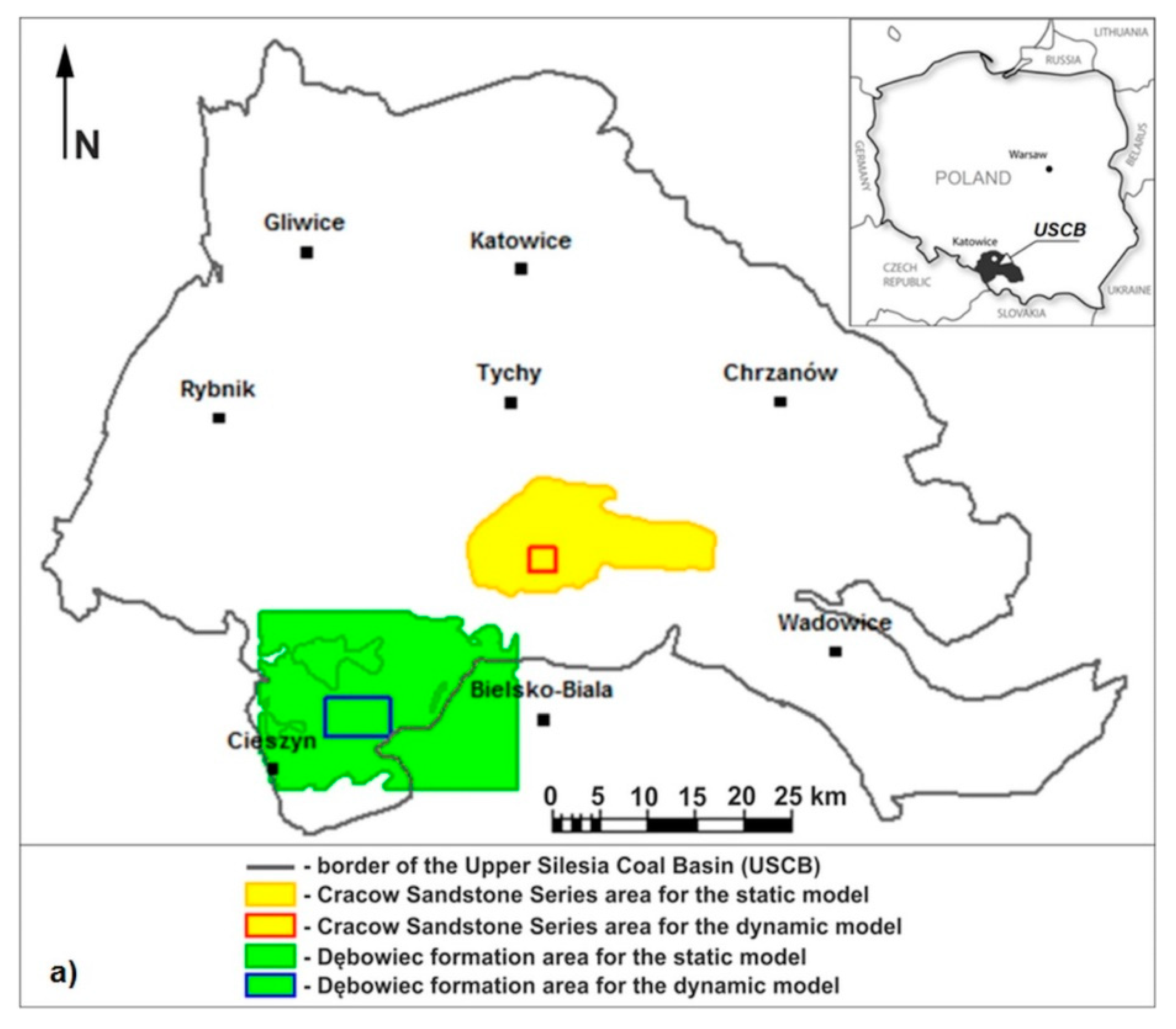
2.1.1. Location of the Study Area
Based on the initial stratigraphic and hydrogeological analysis, the potential for carbon dioxide storage in the USCB area is shown only by two Carboniferous lithostratigraphic complexes - the Upper Silesian Sandstone Series and the Cracow Sandstone Series—as well as the Dębowiec formation, which lies in the bottom part of the Miocene.
Potential geological structures for carbon dioxide storage in the USCB region also include the roof part of the carbonate series (lower Carboniferous) and terrigenous series of the Lower Devonian and Cambrian; however, these series are located at great depths (usually significantly exceeding 2000 m) and are very poorly recognized [
41].
The selected areas are located in the southern part of the USCB. The first area is located in the Cracow Sandstone Series north of Bielsko-Biała (the area of Ćwiklice), while the second area, selected in the Dębowiec formation, is west of Bielsko-Biała (
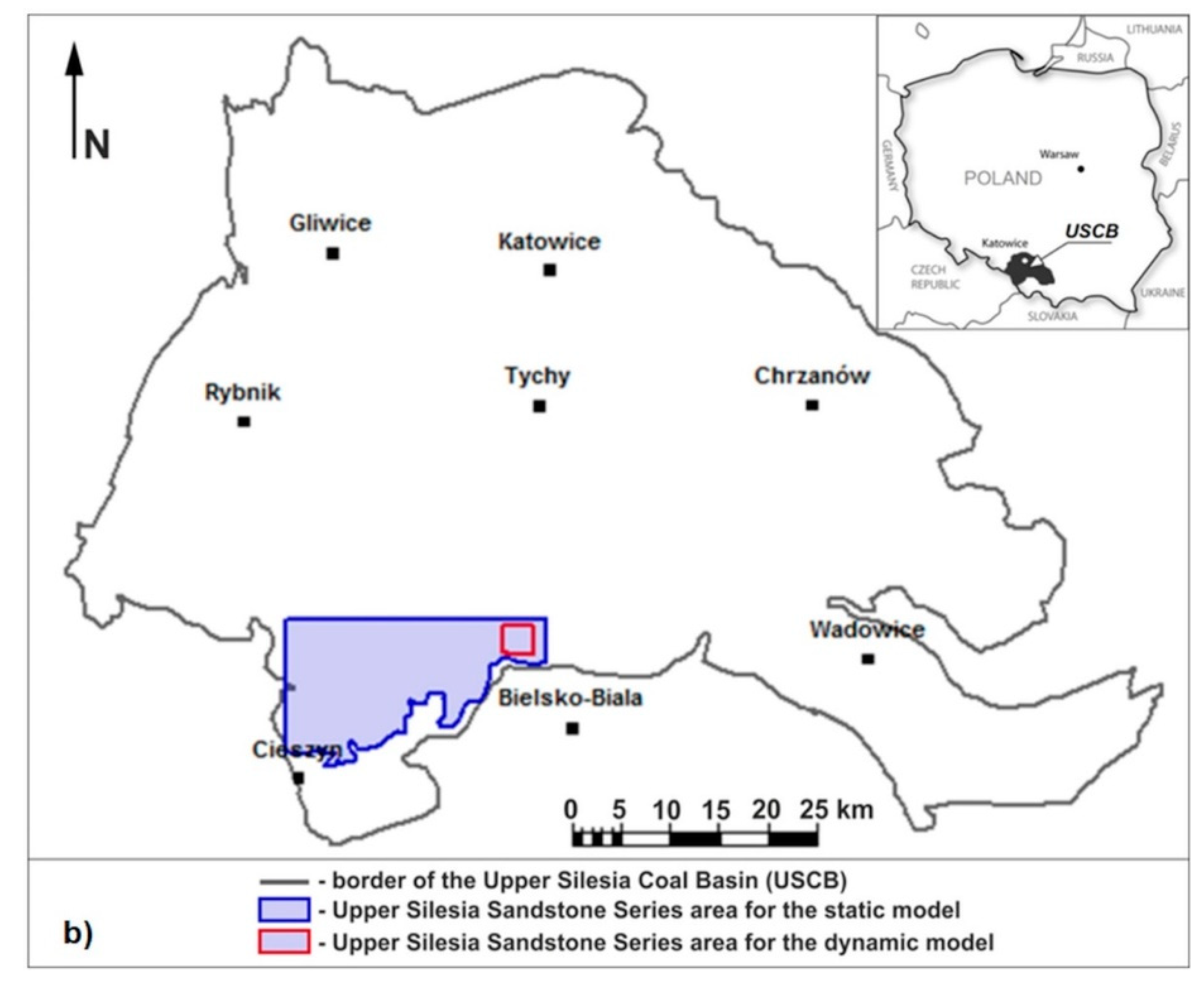
Figure 1a). The third selected region is located within the Upper Silesian Sandstone Series northwest of Bielsko-Biała (
Figure 1b).
3. Results and Discussion
The static regional models for the selected the Upper Silesian Coal Basin (USCB) regions (two Carboniferous lithostratigraphic complexes—the Upper Silesian Sandstone Series and the Cracow Sandstone Series—and the Dębowiec formation) form the basis for constructing detailed dynamic models involving numerical simulations of the process of CO2 injection into potential storage sites.
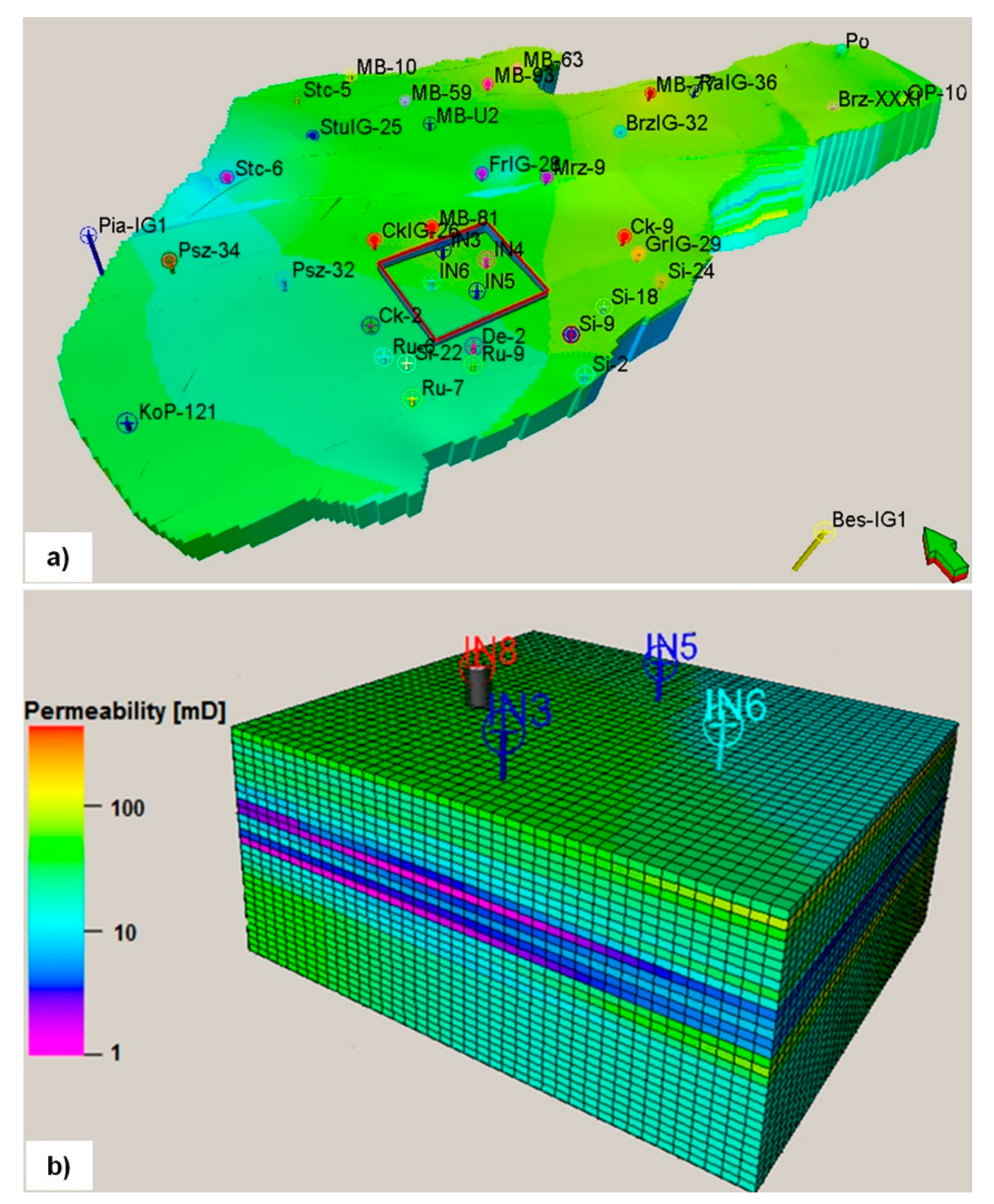
3.1. Numerical Model in the Cracow Sandstone Series Aquifer
Figure 2 presents a static model within the Cracow Sandstone Series. Within the developed model, a local numerical model was selected for which a number of simulations of CO
2 storage processes were carried out.
A model with an area of 7.875 km
2 and a grid resolution of 75 × 75 m was isolated from the initial model (
Figure 2a) with an area of 221.9 km
2 and a grid resolution of 200 × 200 m (
Figure 2b). The detailed characteristics of the local numerical models are summarized in
Table 1.
The effective porosity in the simulation model is in the range of 7.70–21.04%, with an average value of 13.44%. The permeability in the local model, however, ranges from 6.97 mD to 211.36 mD, with an average value of 57.30 mD (
Figure 2b).
In the developed model, four injection wells, namely, IN3, IN4, IN5 and IN6, were used during the simulation, with the injection amount depending on the adopted CO2 injection option.
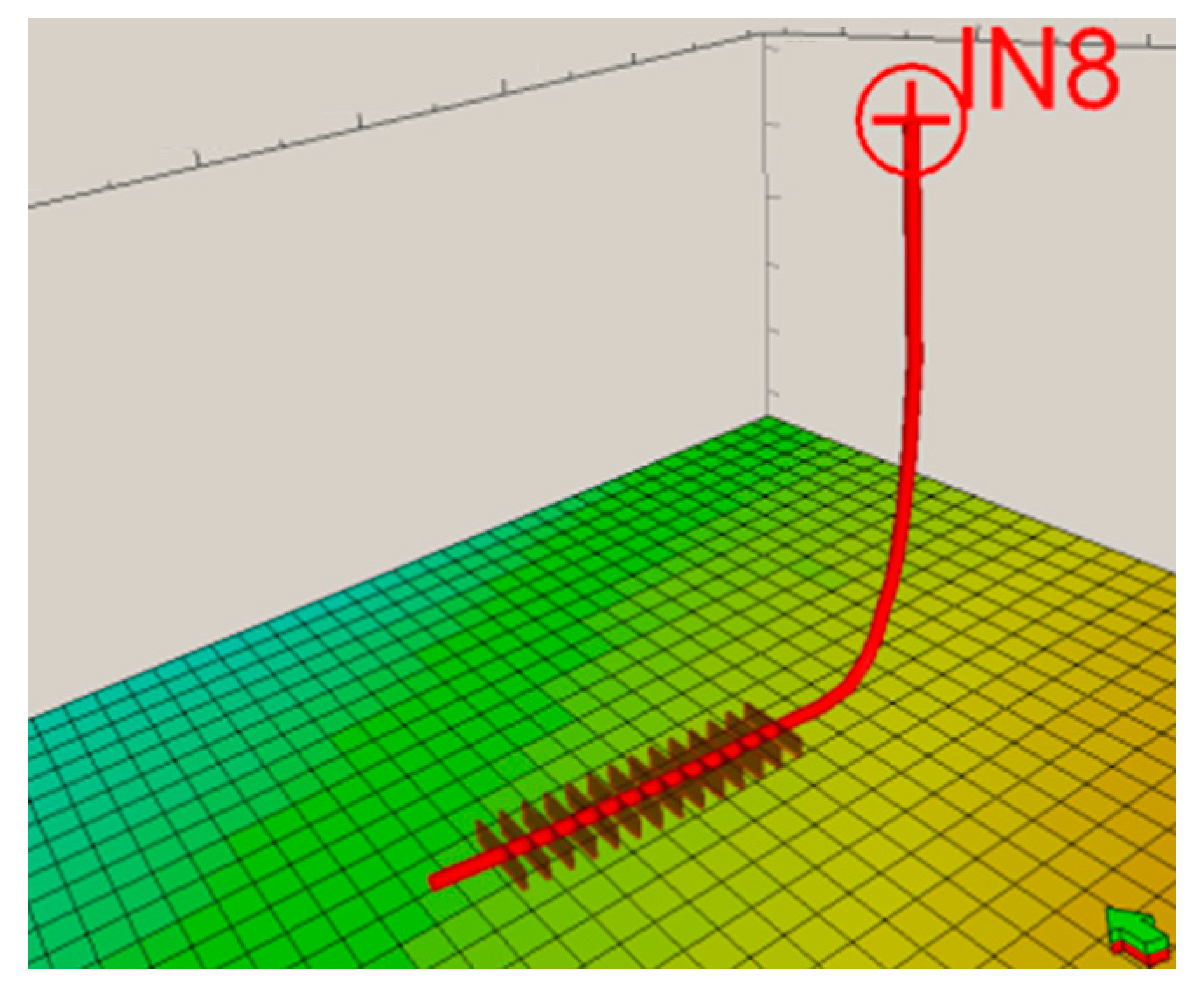
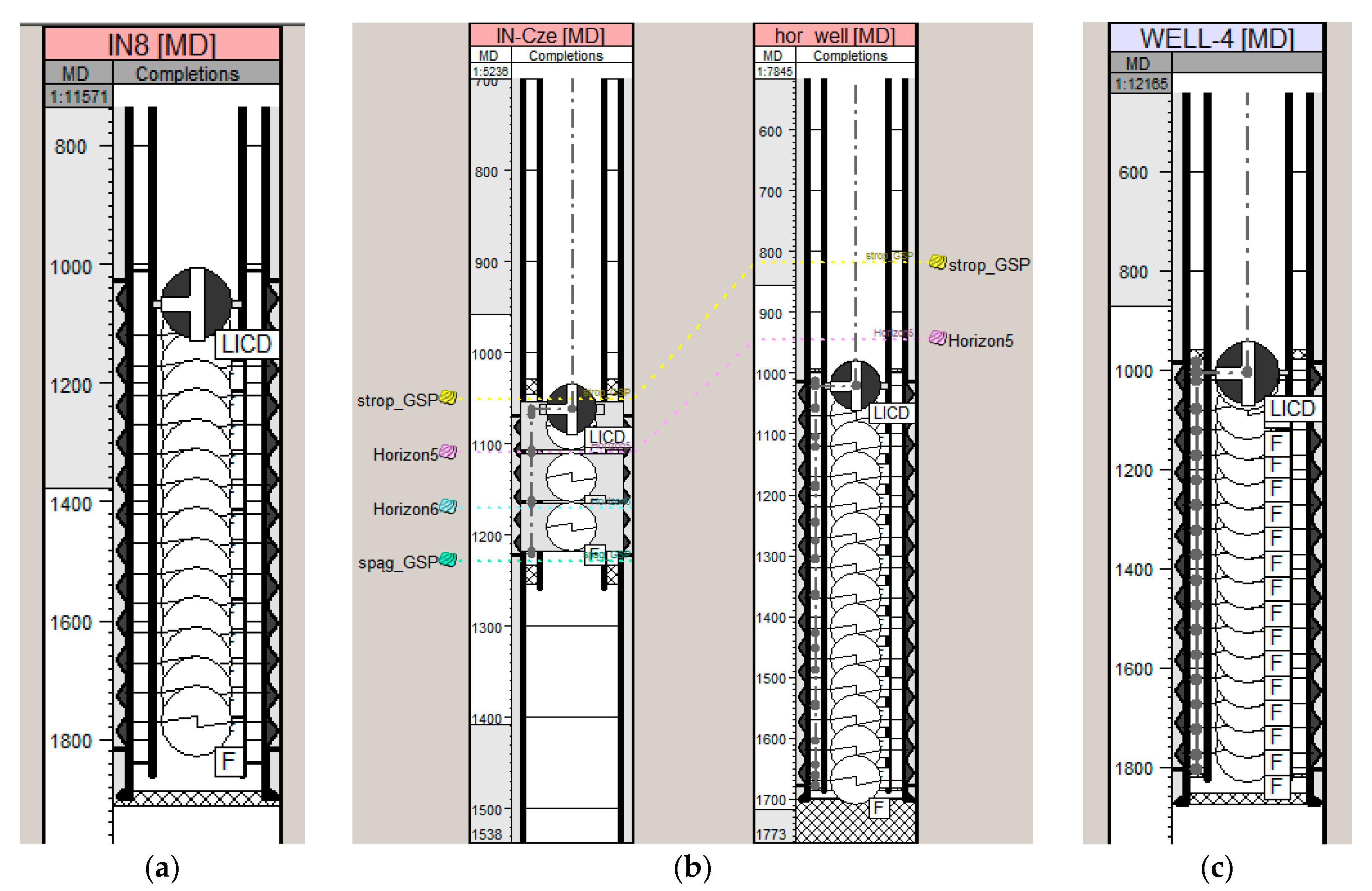
In addition, a single IN-8 horizontal well was designed to simulate the process of CO
2 storage. The behavior of the rock mass during the individual simulation variants after hydraulic fracturing of the rock mass was also considered, aimed at intensifying the CO
2 injection process. Hydraulic fracturing in the horizontal section of the well is shown in
Figure 3.
3.2. Numerical Model in the Upper Silesian Sandstone Series Aquifer
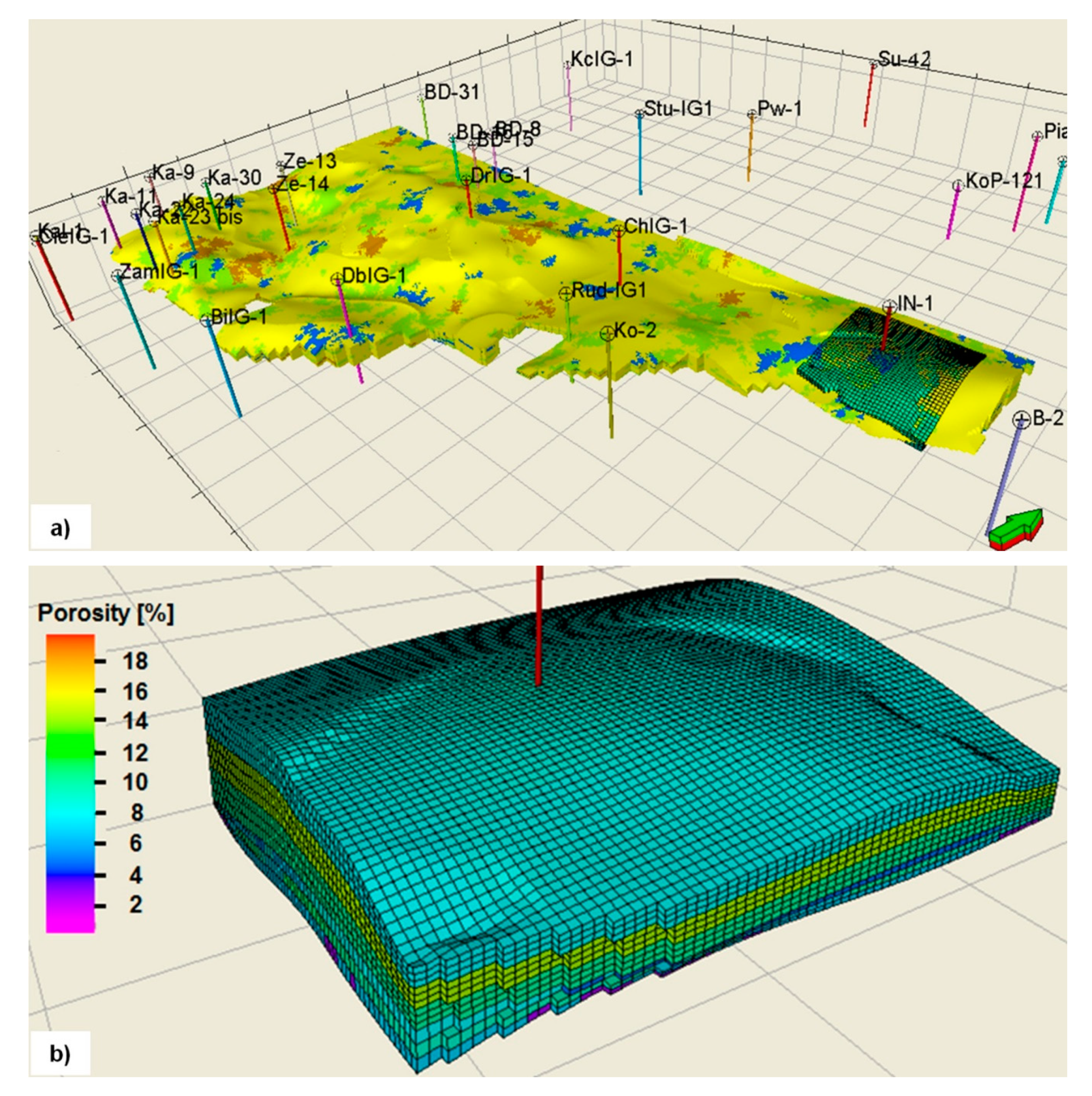
Figure 4a presents a static model built within the Upper Silesian Sandstone Series, together with a local numerical model for which a number of simulations of CO
2 storage processes were carried out.
Based on a model developed on a regional scale (
Figure 4a) with an area of 137.80 km
2 and a horizontal grid resolution of 100 × 100 m, a local model was developed with an area of 9.15 km
2 and a grid resolution of 50 × 50 m (
Figure 4b). A list of detailed characteristics of the local model is presented in
Table 1.
The model implements one vertical injection well located in the central part of the anticlinal structure, as well as a single horizontal well. The values of effective porosity, referring to the interconnected pore volume in the rock structure, in the simulation model range from 2.48% to 16.17%, and for the most part, the average value is approximately 10%. The maximum permeability value in the local model reaches 5.10 mD.
3.3. Numerical Model in the Dębowiec Formation Aquifer
Of the three analyzed reservoirs, the Dębowiec formation is the most prospective for potential storage of CO
2 and is characterized by the most favorable values for the geological and hydrogeological parameters. The Dębowiec formation is a Miocene macroclastic molasse composed of four lithofacies: Olistostromes, boulders, conglomerates and sandstones [
42].
In a static model developed on a regional scale within the rock complex of the Dębowiec formation with an area of 555.75 km
2 (
Figure 5a), a local numerical model with an area of 32.18 km
2 was developed (
Figure 5b), in which a series of numerical simulations of the CO
2 storage process was carried out.
The effective porosity in the constructed simulation model ranged from 6.90% to 14.91%. The maximum permeability value in the local model was 49.88 mD (
Figure 5b).
To simulate the process of CO2 injection into the rock mass, two-directional wells were designed with horizontal section lengths of approximately 500 m and 900 m.
3.4. Models of Reservoir Fluids
At a later stage of the work, reservoir parameters were analyzed in the static models of the selected USCB regions and supplemented with reservoir fluid parameters necessary to simulate CO
2 storage in the studied geological formations and structures. An appropriate simulator module was selected, taking into account the phenomenon of water solubility of CO
2. For this purpose, a compositional version of the ECLIPSE simulator (E300) with the CO2SOL [
43] option was used. The Eclipse reservoir simulator defines the sm
3 unit as a cubic meter of gas at pressure 1 atm = 1013.25 hPa and temperature equal to 15.56 °C. The unit rm
3 describes the volume of gas in the reservoir conditions.
To select the correct state equation and determine the thermodynamic parameters of the process, the Peng-Robinson state equation was used, taking into account the molar volume modification. This equation allowed determination of the thermodynamic parameters in a manner more similar to real conditions [
43]. The viscosity of CO
2 was estimated using the Lorentz-Bray-Clark correlation [
44]. Parameters concerning the solubility of CO
2 in saline were determined from the Chang-Coats-Nolen correlation [
45].
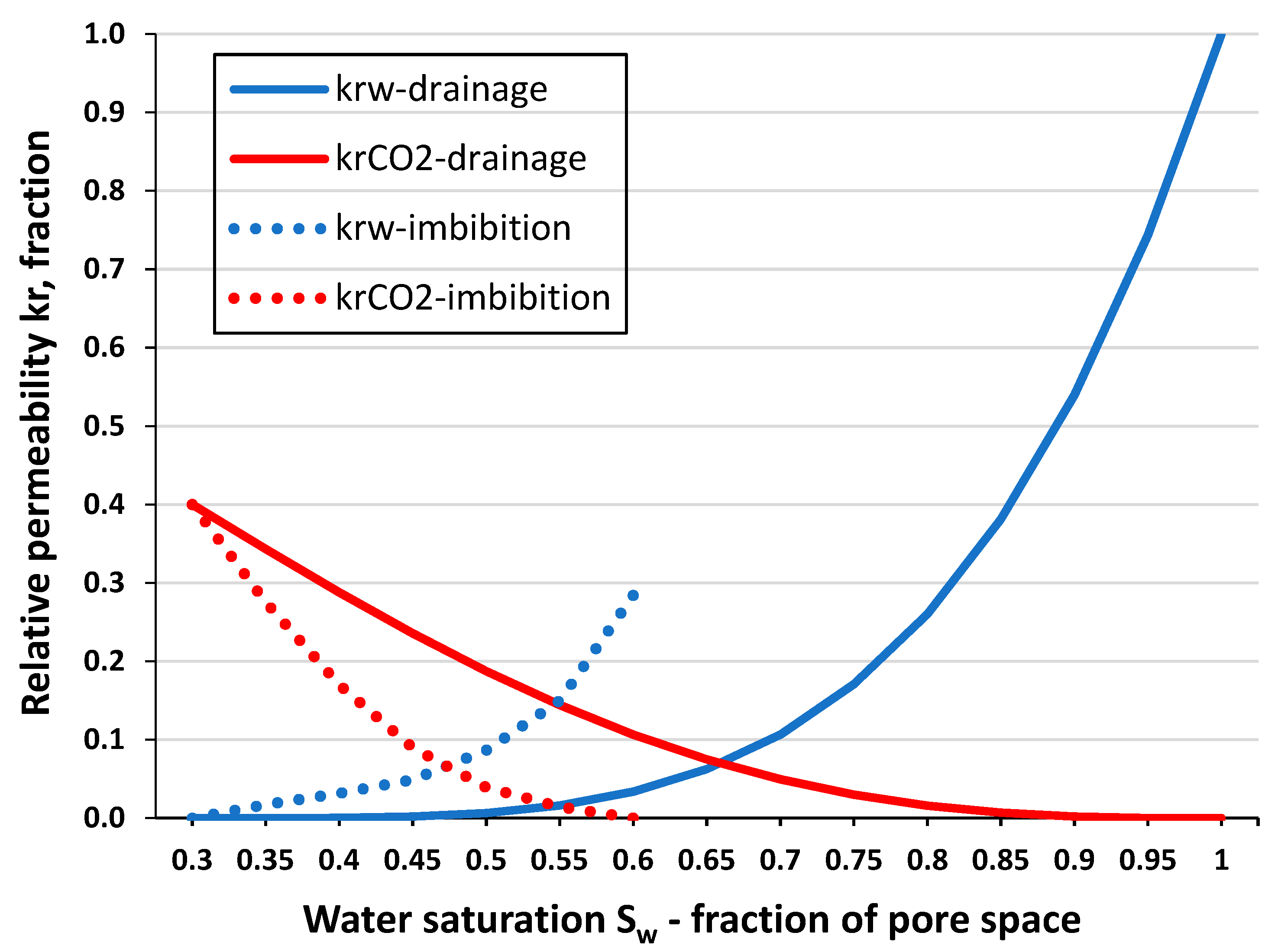
The CO
2 flow in layers saturated with water (brine) is controlled by the curves of relative permeability. In this study, relative permeability curves were generated based on Corey’s correlation [
46]. The often-used Brooks and Corey relations are actually an extension of equations developed by Burdine et al. [
47], for normalized drainage effective permeability. The equations shown here are the original Burdine equations modified for relative permeability calculations:
where:
krw = wetting phase relative permeability;
krn = non-wetting phase relative permeability;
= non-wetting phase relative permeability at irreducible wetting phase saturation;
= normalized wetting phase saturation;
λ = pore size distribution index;
Sm = 1 − Sor(1 − residual non-wetting phase saturation);
Sw = water saturation;
Siw = initial water saturation.
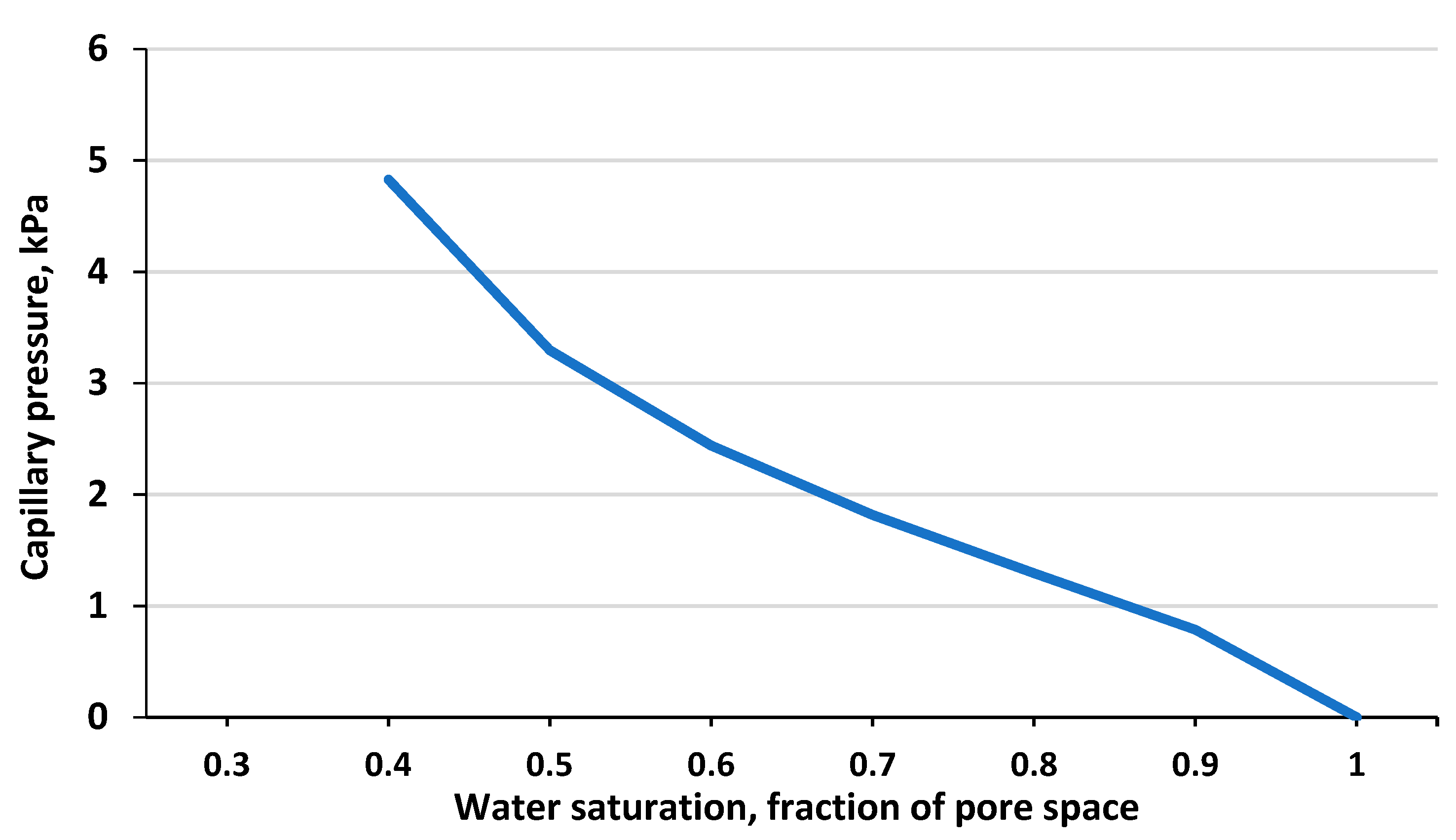
The basic equation for capillary pressure
Pc as a function of liquid saturation is adapted from the van Genuchten formulation [
48], and is given by the following equation:
The values of parameters used in calculations of relative permeability and capillary pressure for simulation models are summarized in
Table 2.
Relative permeabilities relationships as a function of fluids saturation are the key parameters in classical formulations of multiphase flow in porous media. Experimental laboratory tests and an analysis of pore-scale physics demonstrate that relative permeabilities are not single functions of fluid saturations—relative permeabilities display hysteresis effects [
49].
Figure 6 and
Figure 7 shows relative permeability and capillary pressure curves used in the simulation models.
In particular variants of the simulation, the influence of the degree of hydrodynamic openness of the geological structure on the course of the CO
2 storage process was analyzed. Due to the very large surface area of the analyzed geological structures, the aquifers surrounding the area covered by the numerical model were simulated using semianalytic models of aquifers defined by Carter and Tracy [
50].
The surface range of the aquifer models surrounding each simulation variant exceeded the dimensions of the numerically modeled areas several times. In some simulations, the size of the analytical aquifer was defined as the total range of occurrence of a given geological formation (e.g., range of occurrence of the Upper Silesian Sandstone Series in the entire Upper Silesian Coal Basin). The parameters of the above aquifers were defined as mean values from numerically modeled areas. The detailed characteristics of the analytical aquifers are summarized in
Table 3.
As the initial condition of the conducted reservoir simulations, the location of the gas-water contact depth varied in each of the three analyzed models (from 100 m to approximately 170 m). In addition, data regarding the initial reservoir pressure from 10 to 11 MPa (depending on the type of modeled geological formation at depth from 1000 to 1150 m) and temperature were adopted on the basis of archived borehole data. Reservoir fluids at the above pressure and deposit temperature were under hydrostatic equilibrium conditions. The maximum bottom-hole pressures are determined as about 90% of the frac gradient or the leak-off pressure, which represents the pressure that should not be exceeded during CO2 injection, to avoid cover rock failure by fracking.
In this study, the leak-off pressure is approximately 50–60% above the normal hydrostatic gradient. It was assumed in the models that the storage pressure should not exceed 20% of the normal hydrostatic gradient, in order to keep the storage pore pressure way below the leak-off or frac gradient. The basic initial parameters assumed in the individual simulation models are listed in
Table 4.
Constant injection efficiency and the maximum bottom pressure at the injection well PBHP were adopted as the boundary conditions of the analyzed process. These quantities were varied in the individual simulation models depending on the assumed injection variant.
Hydraulic fracturing used in directional drilling is one of the basic operations aimed at improving the parameters of the near-well zone. The main purpose of the fracturing treatment is to increase the rock permeability and to improve the gas exchange between the well and the rock mass. This effect is obtained by creating a system of fractures around the injection section of the well. The radius of the range of fractures is large and can be up to several dozen meters. The formation of fractures in the reservoir rocks is related to the rupture stress being greater than the rock strength limit, generated as a result of the fracturing liquid injected into the well.
The hydraulic fracturing treatment was applied in the case of the directional well for the model of the Cracow Sandstone Series. Fracturing was carried out at 14 depth intervals every 50 meters.
In the model of the Upper Silesian Sandstone Series, the hydraulic fracturing treatment was applied in both the vertical and the horizontal wells. In the case of the vertical well, the fracturing process was initiated at three depth intervals approximately 50 meters apart starting after 30 days from the start of CO2 injection. In the directional well, similar to the fracturing interval in the Cracow Sandstone Series, fracturing was applied at 14 depth intervals every 50 meters.
Simulations of the hydraulic fracturing treatment in the Dębowiec formation model were carried out in a directional well at 16 depth intervals every 50 meters. Schematic arrangement of fracturing intervals in injection wells is shown in
Figure 8. The main properties of fractures assumed in the simulation models are listed in
Table 5.
Simulations of the process of CO2 injection into saline aquifers in the models, including the individual series of sandstone, were made for separate technological variants diversified in terms of the injection methodology applied. The effectiveness of the sequestration process was analyzed in groups concerning the type of injection wells, which means that the use of both vertical wells and the directional (horizontal) well was considered together with the process supported through hydraulic fracturing of the rock mass. In all variants of the simulation, carbon dioxide was injected into the footwall layers of the reservoir. Injection wells with partially perforated casing completion were analyzed. The purpose of the perforation was to achieve the maximum productivity of the opening in a cost-effective manner, and to establish a good connection between the well and the deposit formation.
Different process simulation variants were adopted and varied in terms of injection efficiency. For each of the wells, the injection volume was assumed to be between 1.00 and 3.24 million sm3/d depending on the simulation scenario adopted. In addition, in each of the above variants, the simulation scenarios varied in terms of duration.
Simulations of the CO2 migration process in the analyzed structures were carried out for a time interval of 15 to 400 years after the end of injection (relaxation phase). The duration of the CO2 injection phase was also varied depending on the scenario adopted and ranged from 6 to 25 years.
The influence of the degree of hydrodynamic openness of the structure on the course of the sequestration process was analyzed. The effect of hydraulic fracturing of wells on the injection efficiency was also investigated.
Detailed characteristics of individual injection variants are presented in
Table 6.
3.5. Simulation Results for Model in the Cracow Sandstone Series Aquifer
Simulations of the process of CO
2 injection into saline aquifers in a model, including the Cracow Sandstone Series, were conducted for separate technological variants.
Table 7 presents a list of the modeling results for the total amount of CO
2 injected in the individual simulation variants. The volume of CO
2 is given for regular (sm
3) and reservoir conditions (rm
3).
The largest total amounts of CO2 injected correspond to variant No. 7 (four vertical wells) and variant No. 10 (one horizontal well with fracturing).
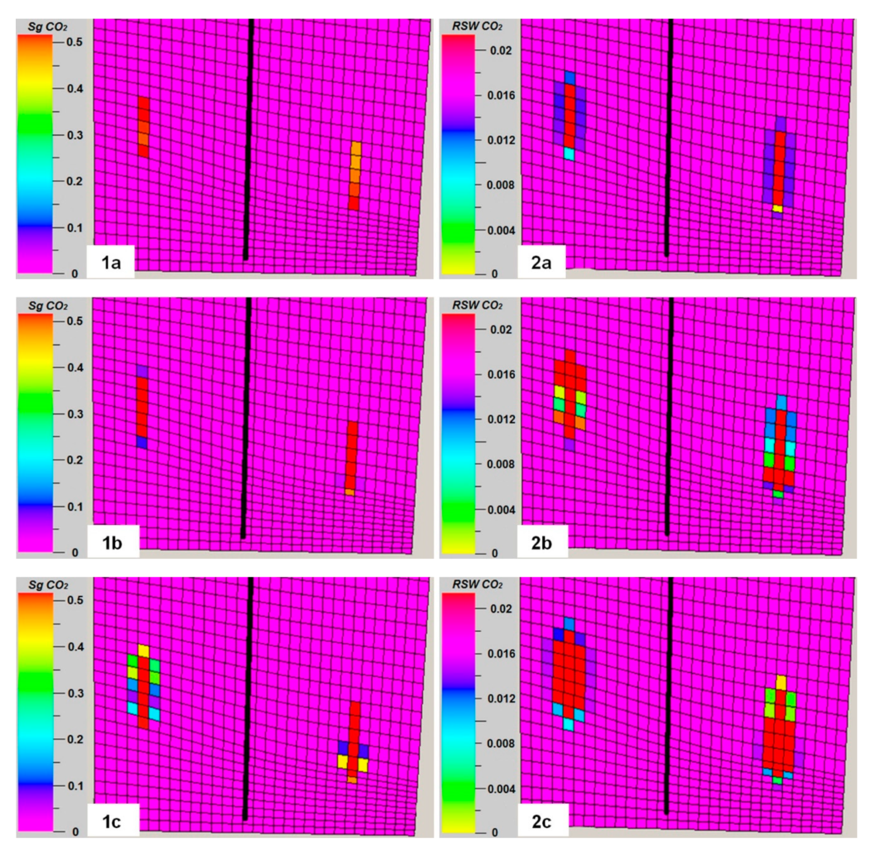
The following figures (
Figure 9) shows the distribution of the saturation of the structure with carbon dioxide remaining in the residual state and the distribution of dissolved CO
2 in the analyzed structure for individual simulation time intervals.
Carbon dioxide in the residual state is defined as the free-phase CO
2 remaining in the nonwetting phase, which after being injected into the rock mass is trapped by capillary forces in the pore spaces of the rocks [
51].
Free CO2 saturation in the aquifer of the Cracow Sandstone Series is presented in the form of a common fraction, while the distribution of CO2 dissolved in the brine is presented in the form of a molar fraction.
In injection variant No. 7 (S7), an increase in is observed, and the maximum is approximately 240 kPa pressure in the roof layers of the aquifer after 25 years of injection. As a result of conducting long-term simulations for the next 400 years from the end of injection, it was found that after approximately 30 years, the reservoir pressure in the structure’s roof is already close to the original pressure before starting the injection of carbon dioxide.
In the initial phase of the simulation, the injected carbon dioxide accumulates in the area of the injection well. Only a slight movement of free CO2 towards the roof layers of the aquifer was observed, probably due to the poor reservoir properties of the analyzed structure. In addition, there is a very slow process of reducing the free CO2 phase, due to the dissolution of CO2 in the brine, which eventually falls to the bottom layers of the aquifer. The phenomenon of brine convection arises as a result of changes in its density caused by the dissolution of CO2.
In injection variant S11 with the use of the directional well, free CO2 zones around the injection well are also formed and gradually develop. There is also a noticeable slow movement of CO2 towards the aquifer’s roof layers, due to the dominant buoyancy forces. In addition, there is a phenomenon of dissolution of CO2 in the brine, and descent of dissolved CO2 towards the lower layers of the aquifer. It can be observed that the brine containing dissolved CO2 spreads over a much larger area than the residual CO2 zone. It is caused by a gradual disappearance of residual CO2, due to its dissolution in brine.
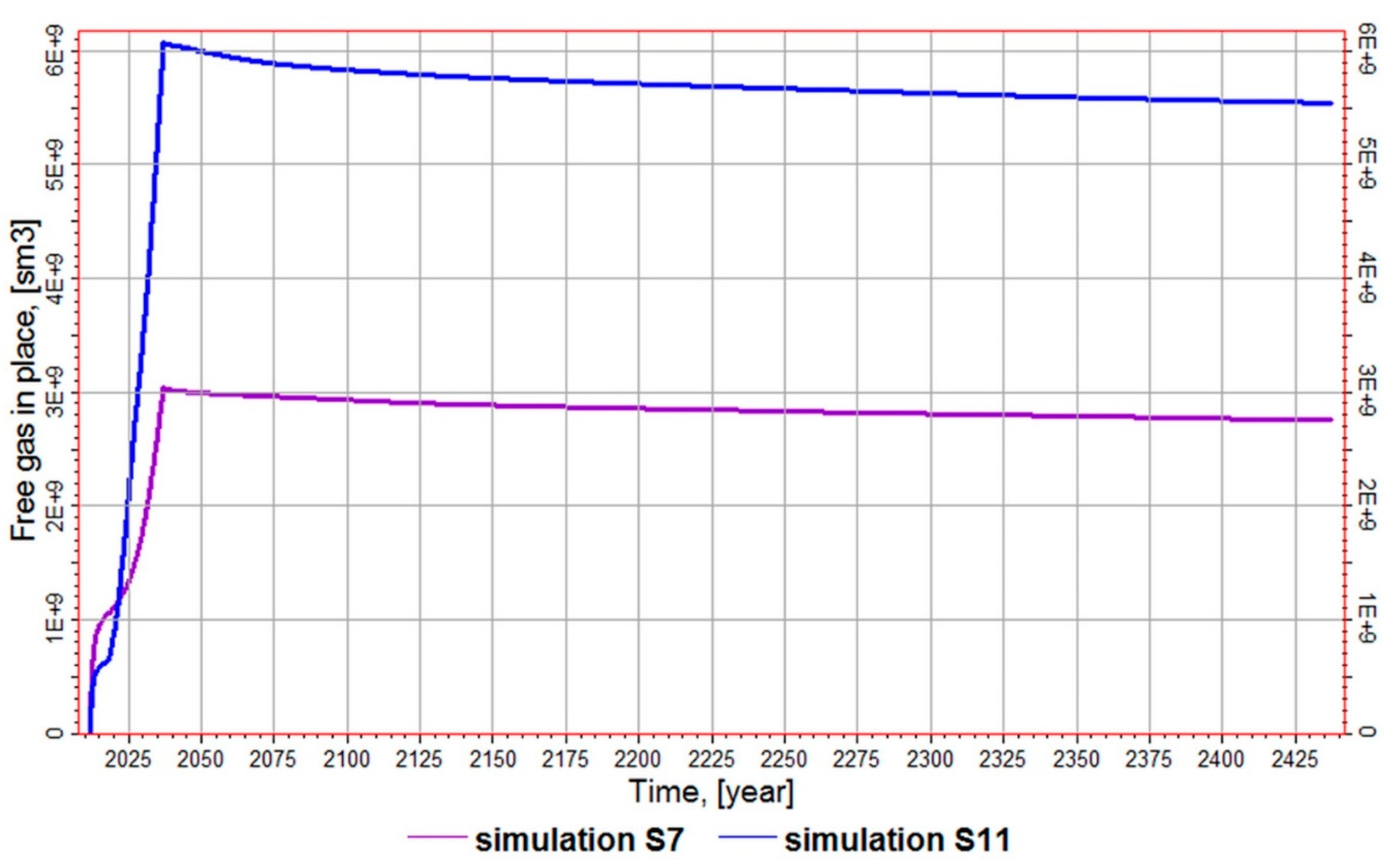
Figure 10 presents the course of the free-phase CO
2 reduction process due to the dissolution of CO
2 in brine in the two injection variants previously analyzed (S7 and S11). In the simulation scenario with a directional well, the reduction of free CO
2 in the structure is faster—there is a dissolution of approximately 500 million sm
3 of CO
2 in the zone of the directional well in relation to approximately 300 million sm
3 of CO
2 in the zone of the vertical well. In the case of a directional well, the process of dissolution of injected CO
2 in the brine is more effective, due to the much larger contact zone of carbon dioxide with unsaturated brine. The efficiency of the dissolution process strongly depends on the effective surface area of the contact of CO
2 with the brine.
3.6. Simulation Results for Model in the Upper Silesian Sandstone Series Aquifer
Simulations of CO
2 injection into saline aquifers in a model of the Upper Silesian Sandstone Series were conducted for separate technological variants. Calculations were carried out for eight simulation variants using one vertical well and two variants including injection with a directional well with the process supported by hydraulic fracturing of the rock mass.
Table 8 presents a list of the modeling results for the total amount of CO
2 injected in the individual simulation variants.
In the first two variants of the simulation, the maximum bottom pressure was set in the injection wells at PBHP = 12 MPa, while in the other variants, the bottom pressure was assumed to be equal to PBHP = 15 MPa. The first two variants compared CO2 injection for a period of 10 years, investigating the impact of fracturing in a single well on injection efficiency. Application of hydraulic fracturing enabled injection of almost twice as much CO2 in comparison to the amount of CO2 injected without fracturing.
In the next three variants (S3, S4, S5), the influence of degree of hydrodynamic openness of the structure on the sequestration process was investigated. After taking into account in the simulation the aquifers surrounding the structure area covered by the model, only a slight increase in the total amount of CO2 injected (S4) was found. The increase in the size of the surrounding aquifer to the size of the Upper Silesian Sandstone Series in the entire USCB did not affect the amount of injected CO2 (S5). The size of the analytical aquifer has no real influence on the efficiency of CO2 storage probably due to a small amount of CO2 that managed to inject in these three simulations (S3, S4, S5).
In variant No. 8, the injection of carbon dioxide was stimulated by hydraulic fracturing. This variant resulted in an increase in the amount of CO2 injected to a value of approximately 1.243 million Mg CO2 (1.243 Mt CO2). Increasing the assumed injection efficiency up to 3 million sm3/d in variant S9 resulted from an attempt to achieve maximum productivity of the injection wells. This change did not give the expected outcomes, and as a result, values similar to those in variant S8 were obtained, probably due to the poor reservoir properties of the analyzed structure. Additionally, in variant S10, after taking into account in the simulation the aquifers surrounding the structure area covered by the model, only a slight increase in the total amount of injected CO2 was found.
In the last variant of the simulation (S11), the sequestration process carried out using the horizontal well with fracturing was investigated. The pressure characteristic of the sequestration process was registered during the simulations. Similar to the previous model, the pressure at the bottom of the injection well reaches the assumed maximum value in the course of injection. Then, it drops rapidly after the injection is completed, and—in the next stage of the simulation—the aim is to achieve the initial pressure.
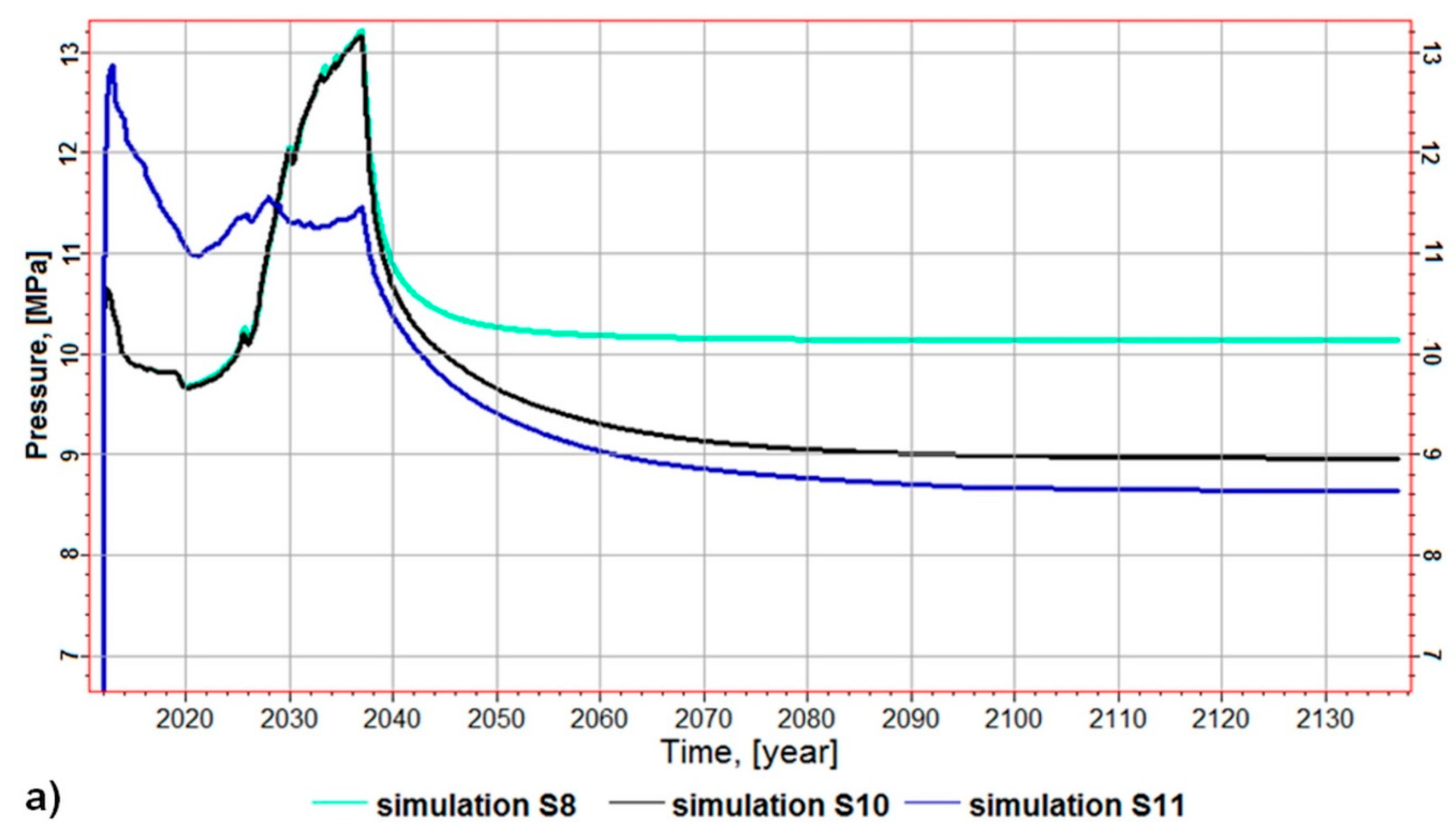
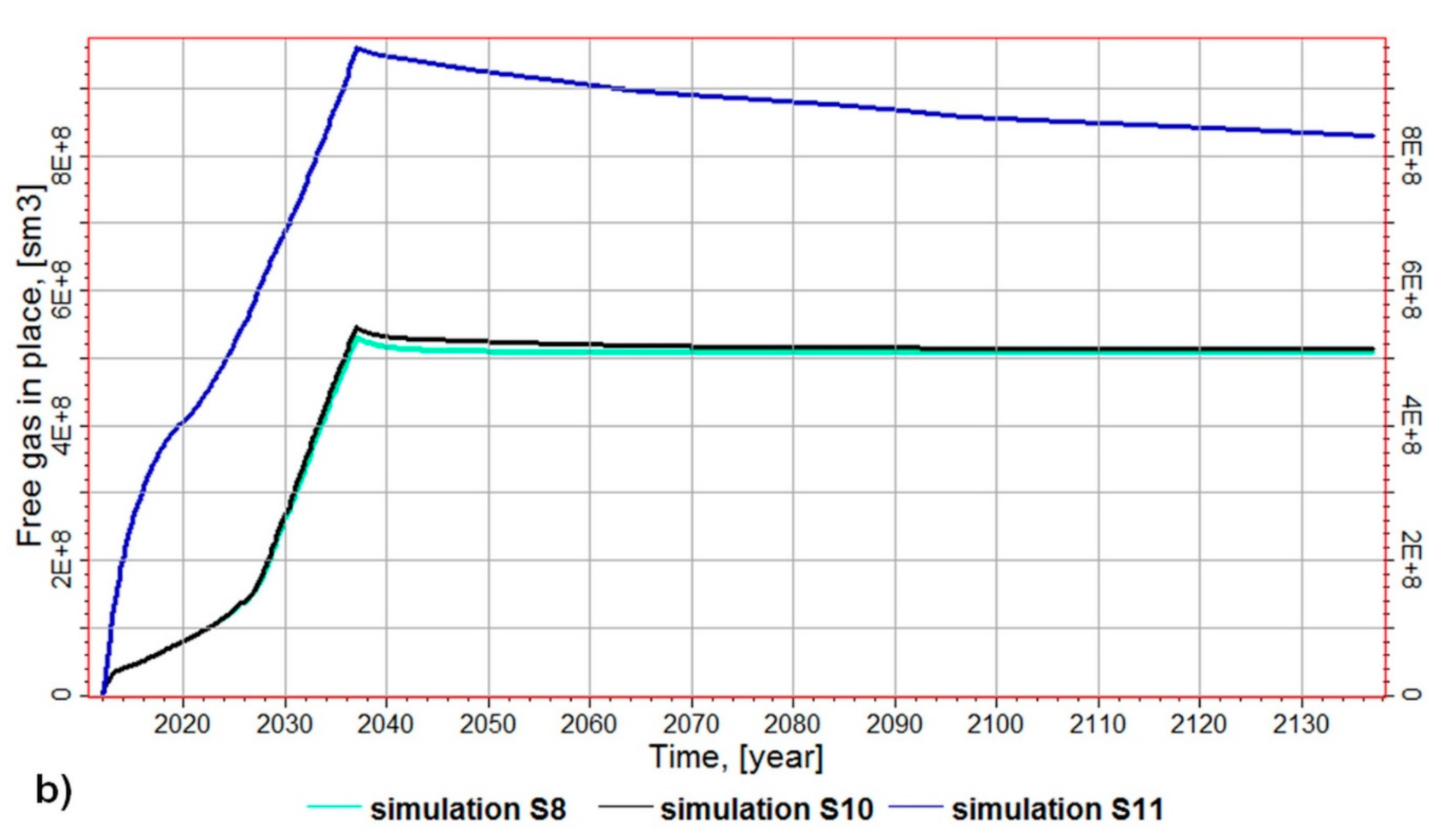
Figure 11a presents the course of changes in average pressure in the injection zone for three simulation variants (S8, S10, S11). In the case of variant 10, the highest total amount of injected CO
2 was obtained from all simulations, including injection into a vertical well. The results of this simulation were compared with the results of a simulation involving carbon dioxide injection using a horizontal well (S11).
Figure 11b shows the dissolution rate of injected CO
2 in brine for the two simulation scenarios. Similar to the previous model, the course of the dissolution process of CO
2 in brine in the variant with a vertical borehole is negligible, while simulation with a horizontal borehole is already characterized by the highly dynamic dissolution of CO
2 in brine.
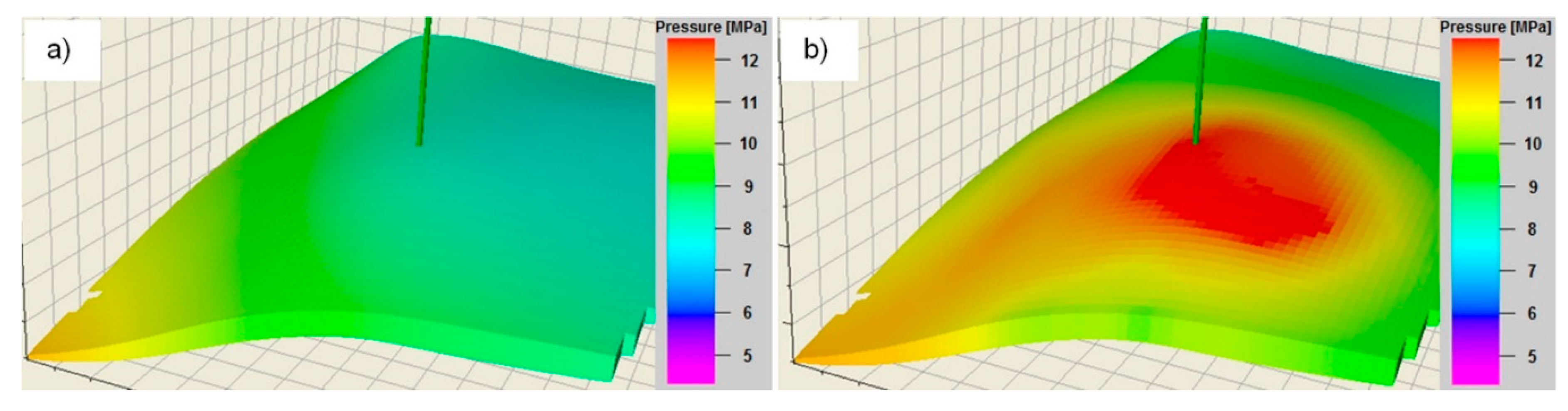
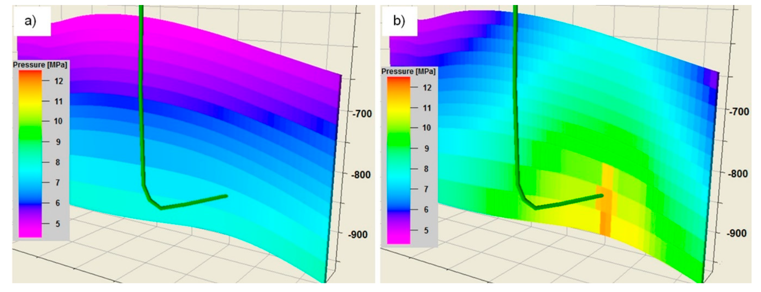
In the simulation carried out according to the S11 scenario, a significant increase in pressure in the roof layers of the aquifer after the end of injection in relation to the initial pressure was observed, amounting to a maximum of approximately 4.7 MPa after 25 years of injection (
Figure 12 and
Figure 13).
Such a significant excess of pressure on the roof of the structure, constituting the amount limiting the effective capacity of the CO2 storage process, resulted in the unsealing of the overburden rocks and partial leakage of CO2 into the superficial layers belonging to the mudstone series. After the injection of carbon dioxide, a pressure drop in the roof layers is visible; however, as a result of long-term simulations after even 400 years, there is still a pressure surge of approximately 1.15 MPa relative to the original pressure in the structure’s roof.
In the S12 scenario, the formation and gradual development of free CO
2 zones occur around the injection well. It is also noticeable that CO
2 moves towards the roof layers of the aquifer and further towards the local top of the structure, due to the dominant buoyancy forces. In addition, there is a phenomenon of dissolution of CO
2 in brine.
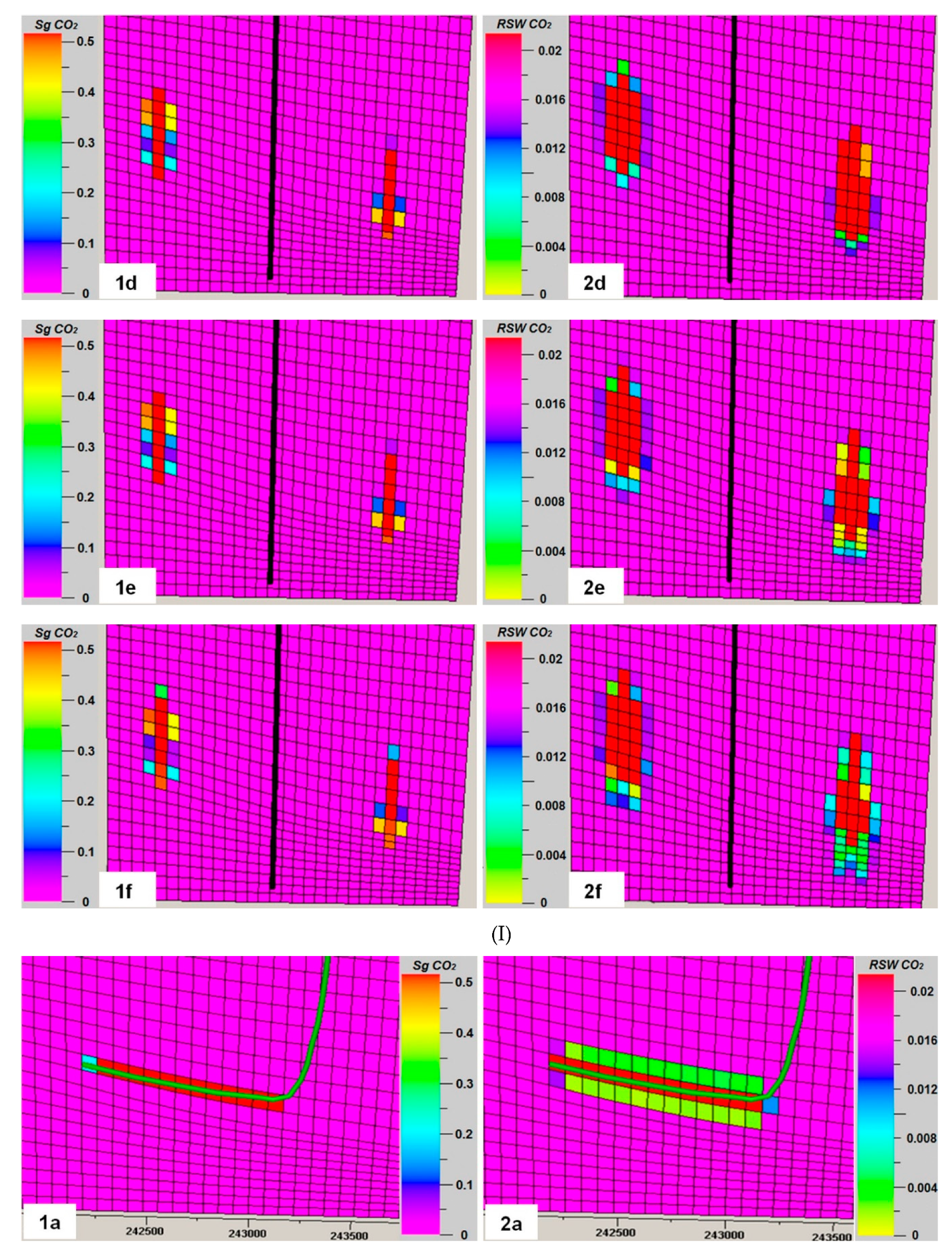
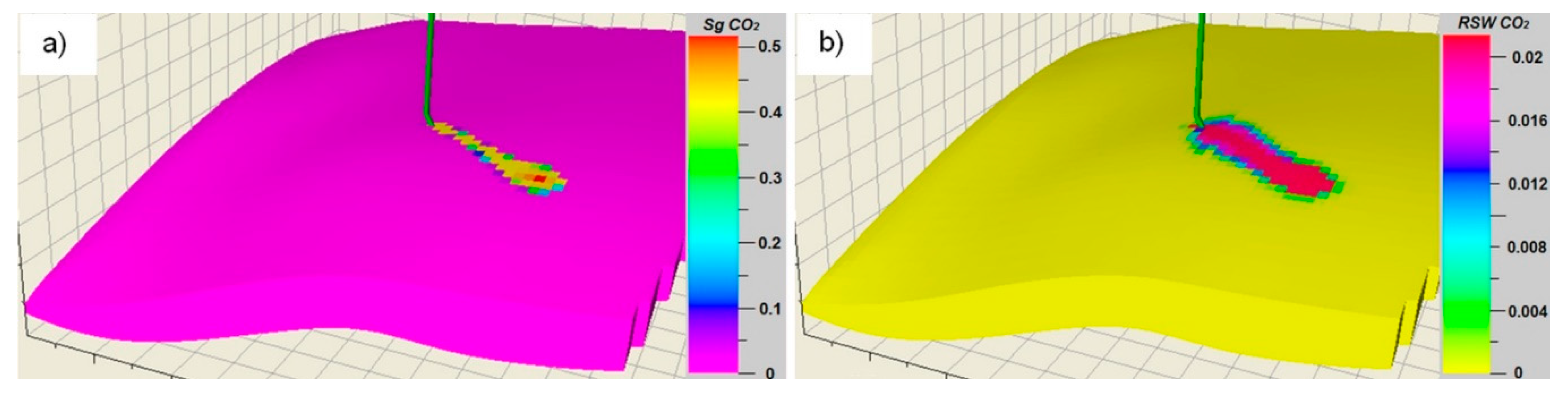
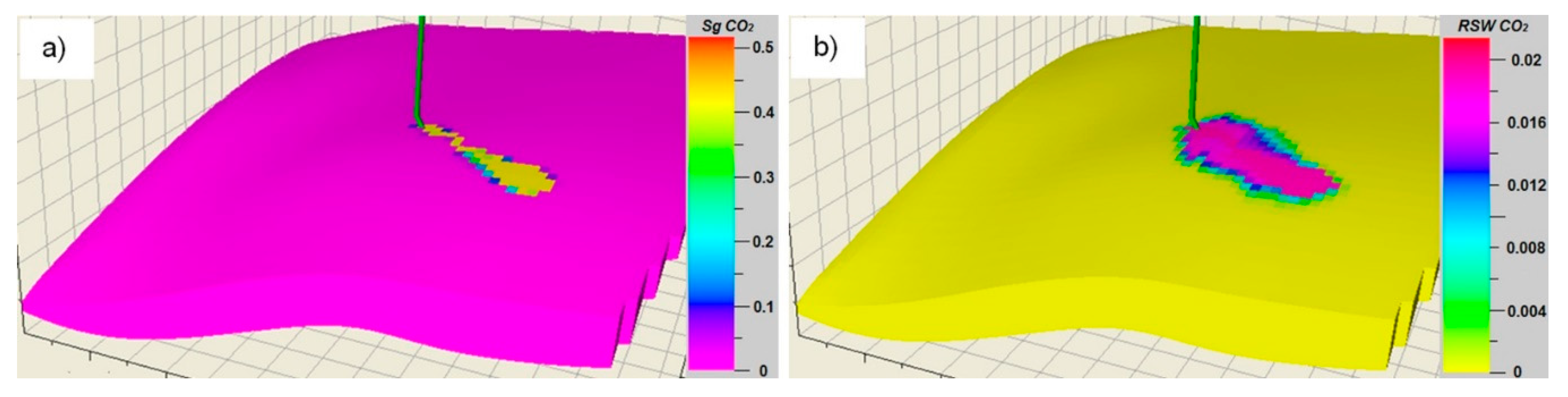
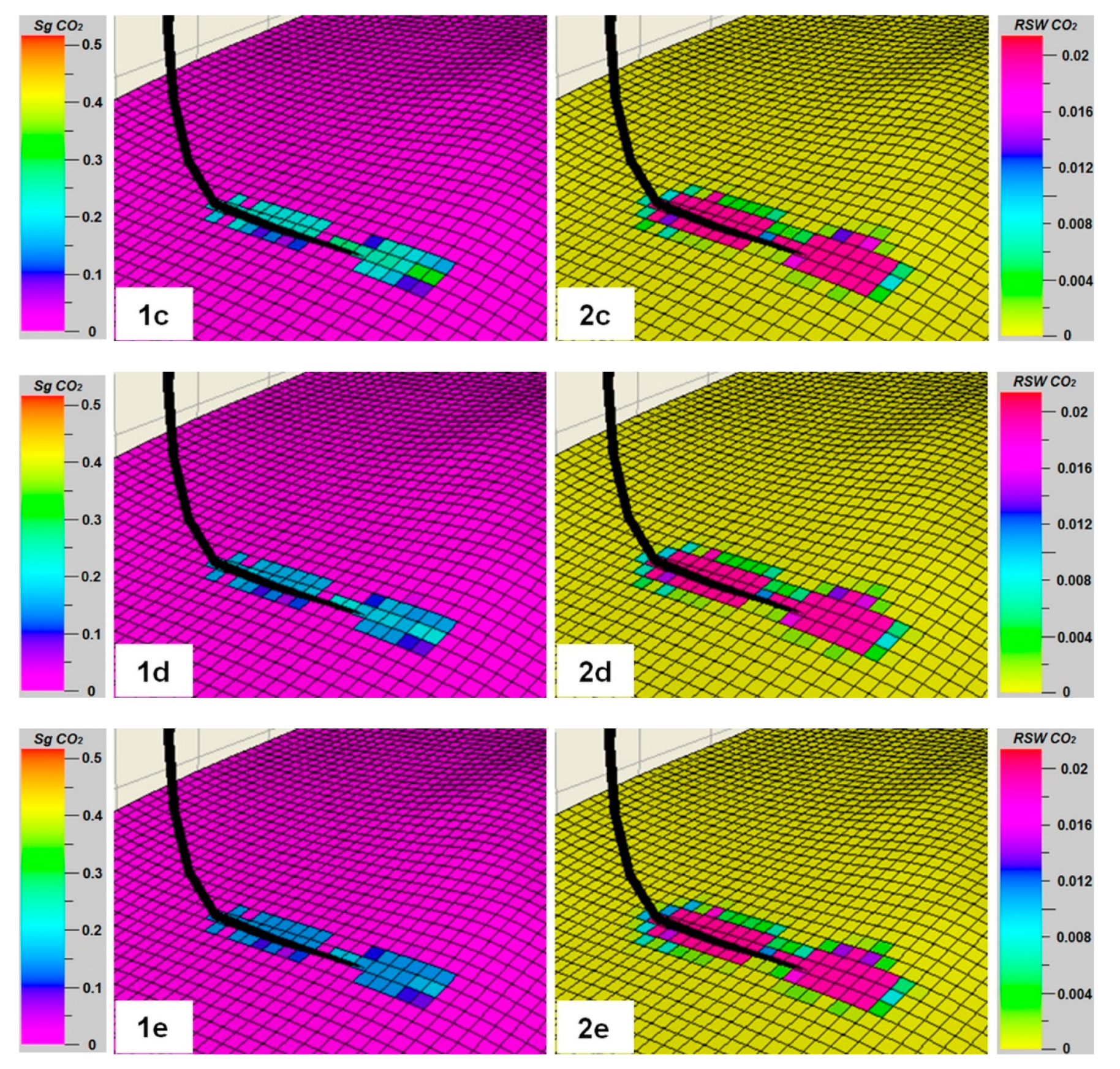
Figure 14 presents changes in free CO
2 saturation and dissolved CO
2 in the roof part of the injection layer after 25 years of injection, whereas
Figure 15 shows changes in CO
2 saturation after 200 years from the end of injection. It was found that the brine containing dissolved CO
2 spreads to a much larger area than the zone of residual CO
2.
3.7. Simulation Results for Model of the Dębowiec Formation Aquifer
The analysis of the geological CO2 storage potential in the Dębowiec formation included three selected simulation variants that show the greatest efficiency of CO2 storage in the rock mass while maintaining injection parameters that ensure safe storage.
Simulations of the process of CO
2 injection into aquifers in the model, including the Dębowiec formation, were made for three variants, of which one included injection of CO
2 with a directional well with the process supported through hydraulic fracturing of the rock mass.
Table 9 presents a list of the modeling results for the total amount of CO
2 injected in the individual simulation variants. As with the previous model, the volume of CO
2 was given for regular and reservoir conditions.
Based on the initial reservoir pressure and previously conducted test simulations, it was found that to enable effective CO2 injection for the assumed 25-year period, the bottom-hole pressure value in the injection well should not be higher than PBHP = 13 MPa.
In the first variant of the simulation (S3A), CO2 injection is continuous for 25 years using a directional well, with the length of the horizontal section equal to 500 m.
In the second variant of the simulation (S4), CO2 injection is also continuous for 25 years using a directional well, with the length of the horizontal section equal to 900 m.
In the case of the third simulation scenario of the CO2 storage process in the Dębowiec formation (S5A), CO2 injection was supported through hydraulic fracturing of the rock mass. Here, CO2 injection was assumed for 25 years with an injection rate of 2.5 million sm3/d.
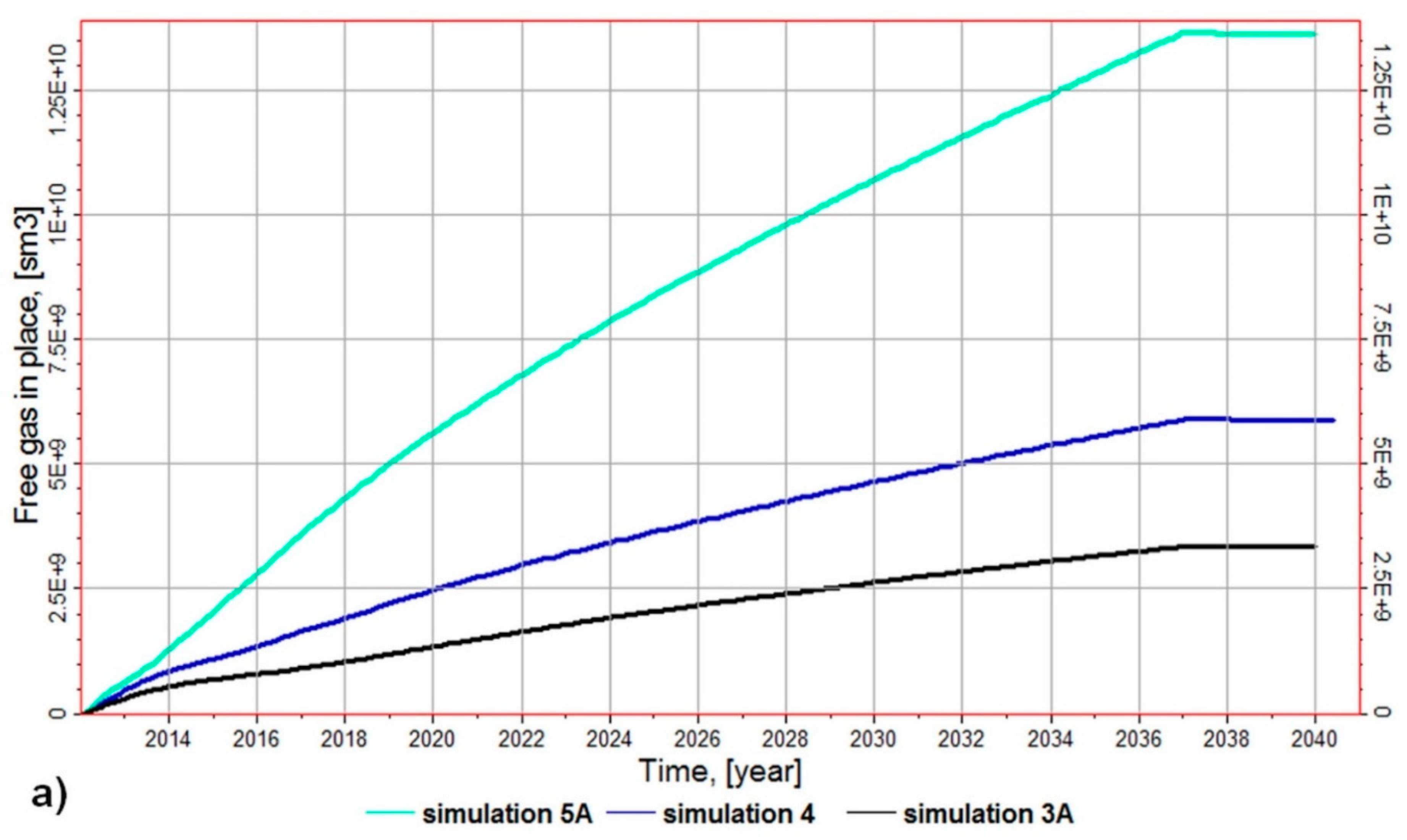
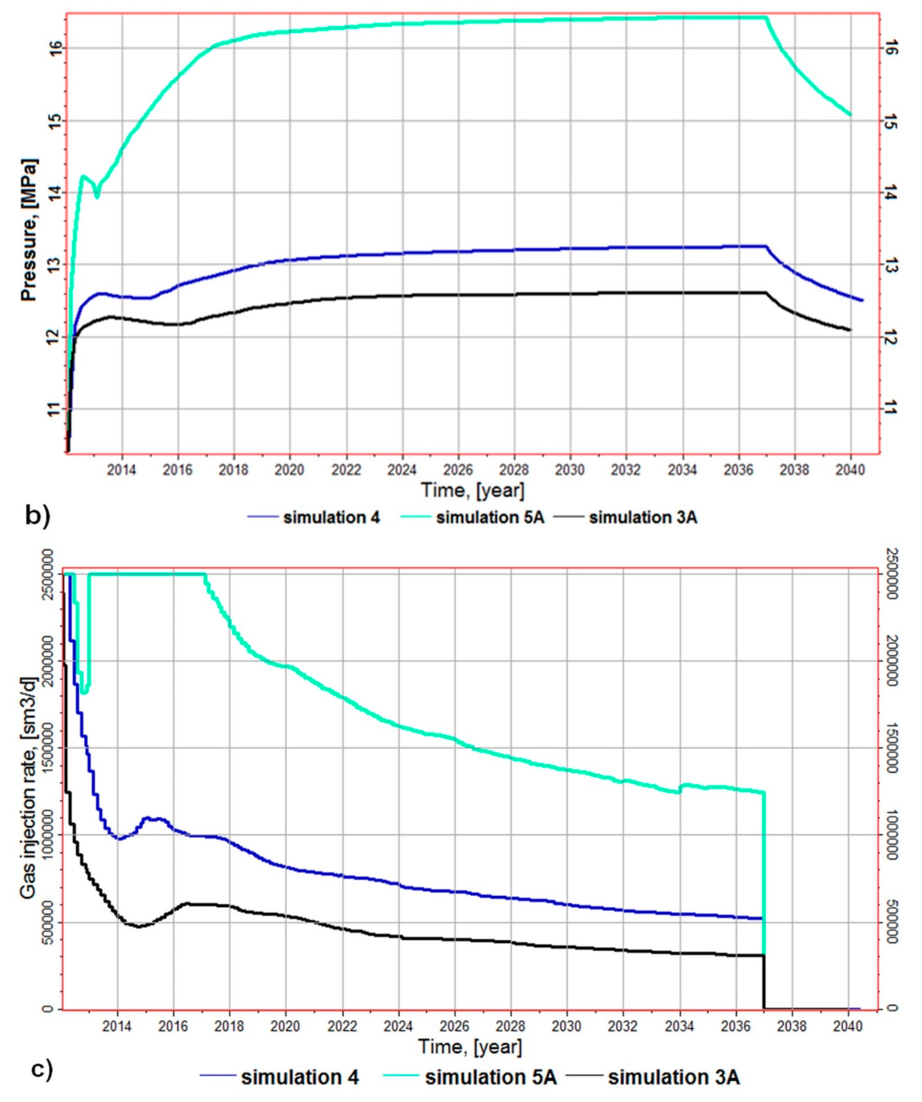
Figure 16 presents the total amount of CO
2 injected into the rock mass as a function of time in individual simulation variants (
Figure 16a), changes in the average pressure in the injection zone (
Figure 16b) and changes in the injection efficiency in particular simulation variants (
Figure 16c).
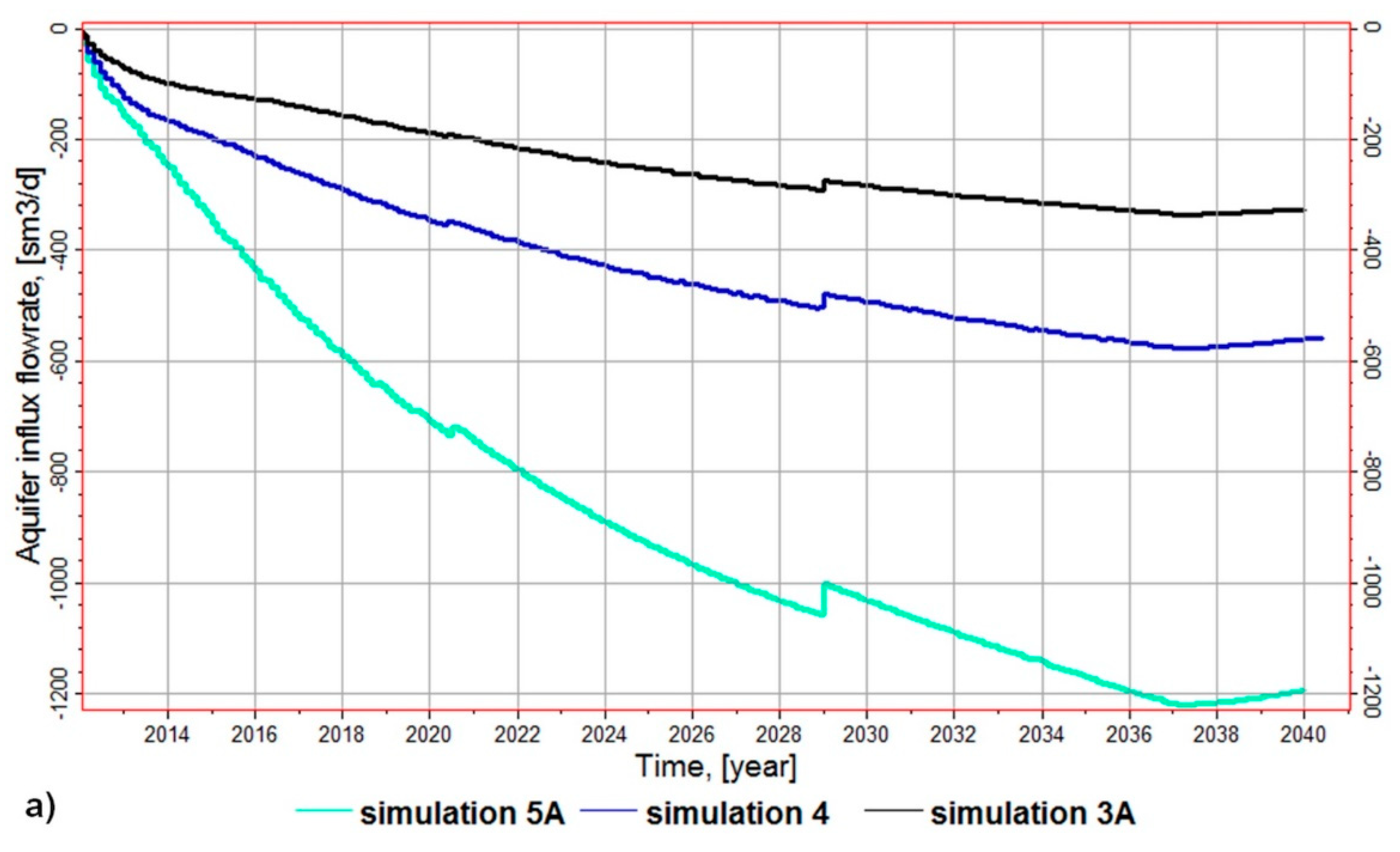
The process of CO
2 injection into the geological formation is usually divided into CO
2 drainage and water imbibition stages. During the drainage process, the gas saturation increases and CO
2 displaces brine when it is injected into the geological formation. An outflow of water from the aquifer can be observed during the injection process, which varied according to the variant of the simulation (
Figure 17a). The largest water movement in the analytical aquifer was found in variant S5A.
As the injected CO
2 is driven upward to the top of the aquifer, due to buoyancy forces, ambient groundwater flows into brine formation. This replacement of CO
2 by groundwater behind the rising CO
2 plume is an imbibition process [
52]. Therefore, a small inflow of water can be observed after the end of the process of CO
2 injection (
Figure 16a). In this stage, capillary trapping of the CO
2 is an essential mechanism after the injection phase during the lateral and upward migration of the CO
2 plume. Once the injection stops, the CO
2 continues to migrate upward to the top of the aquifer. Gas continues to displace water in a drainage process (increasing gas saturation) at the leading edge of the CO
2 plume. Meanwhile, water displaces gas in an imbibition process (increasing water saturations) at the trailing edge of the CO
2 plume. Finally, the presence of an imbibition saturation leads to trapping of the gas phase [
49].
It is related to the effect of the hysteresis in the relative permeability that has an important influence on CO2 trapping. After the CO2 injection is completed, during the imbibition phase, the water displaced by CO2 starts to return and displace the carbon dioxide, at the same time cutting off the smaller pore channels saturated with supercritical CO2. Residual gas is trapped after the end of CO2 injection when water displaces CO2. As a result, a part of the migrating CO2 remains immovable within the pore space by surface forces (e.g., capillary, buoyancy and viscous forces).
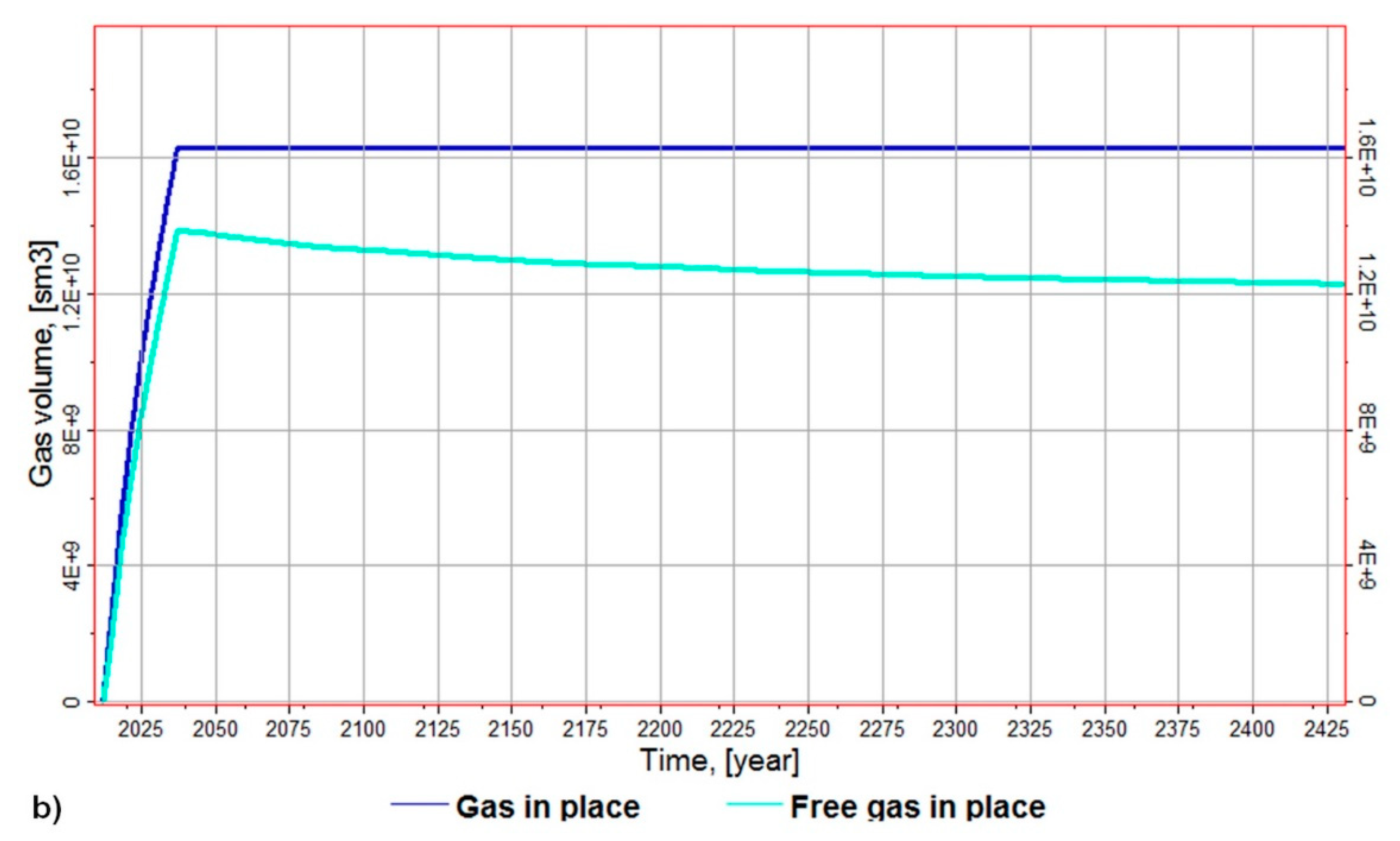
Similar to the previous models, this simulation case indicates a slow process of reducing the free-phase CO
2, due to its dissolution in the brine, while maintaining a constant amount of CO
2 (Gas in place) in the formation (
Figure 17b).
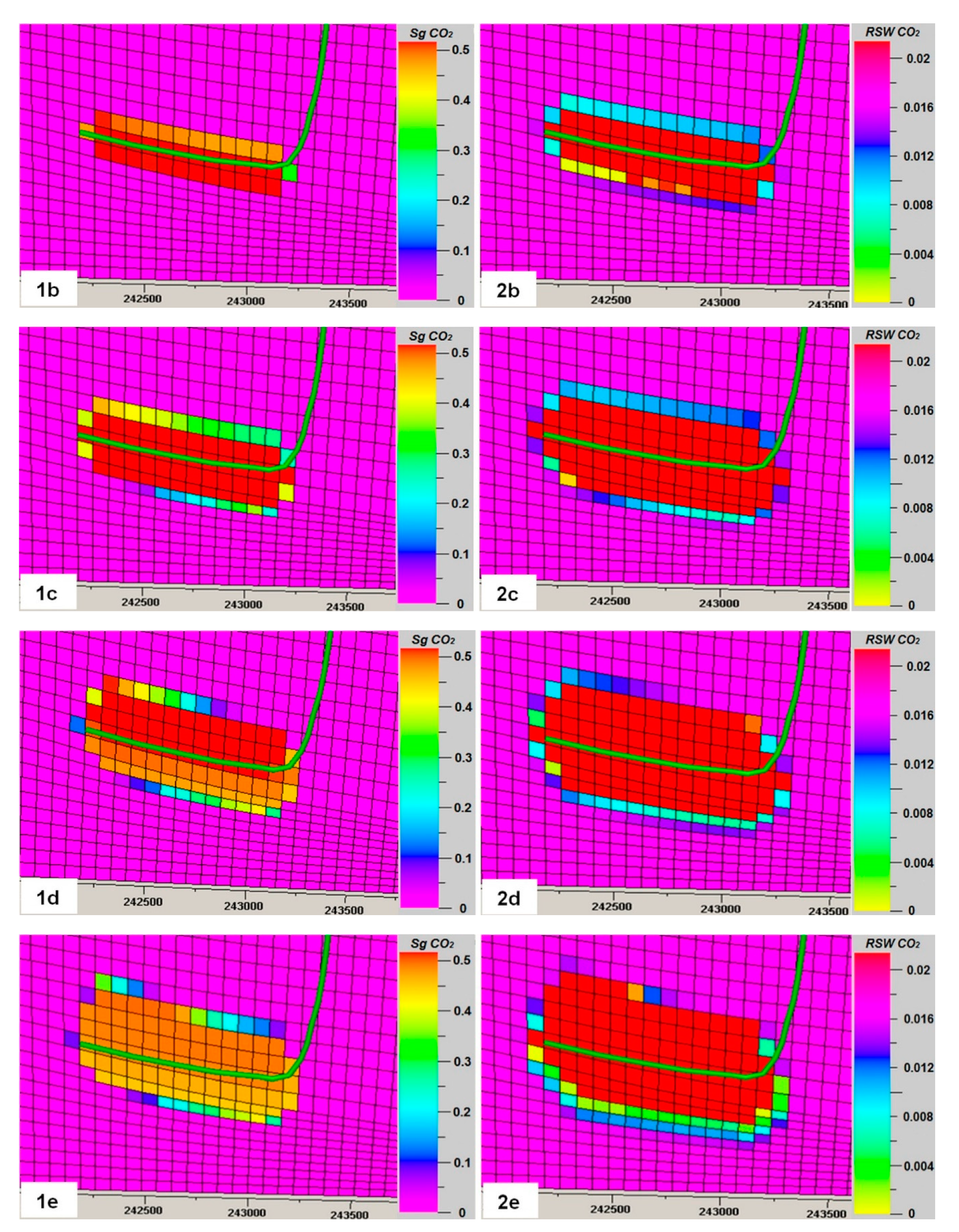
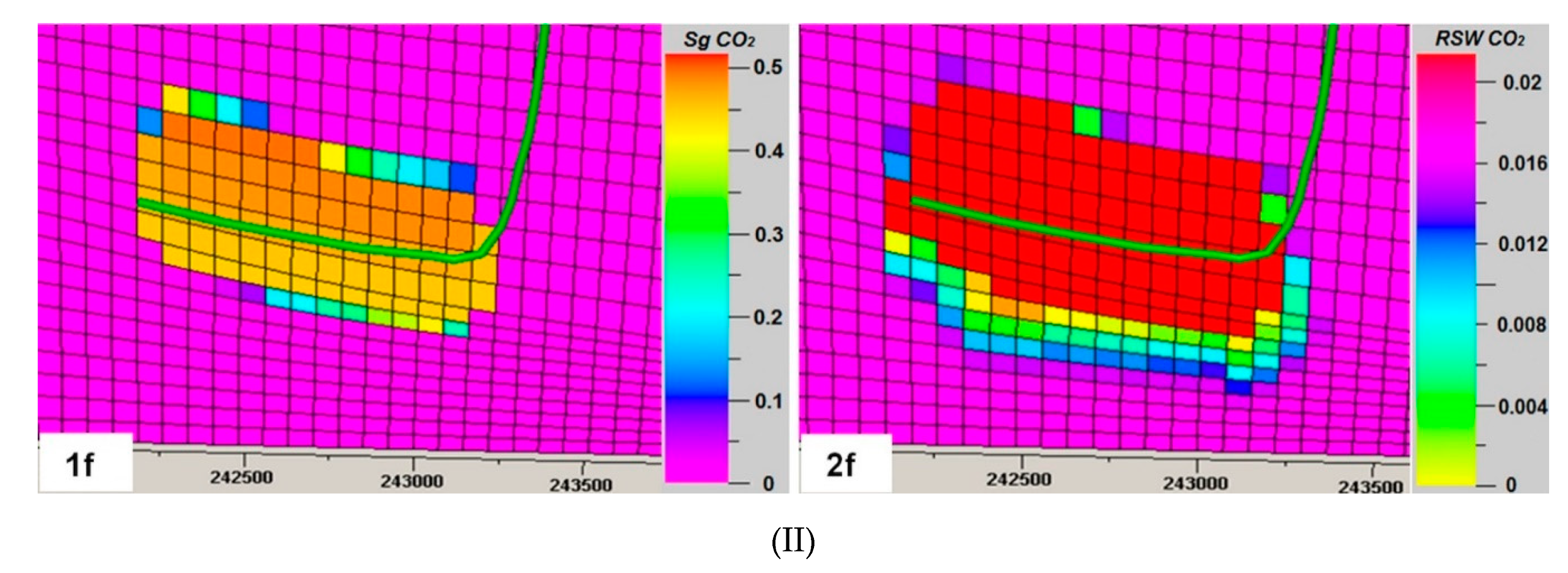
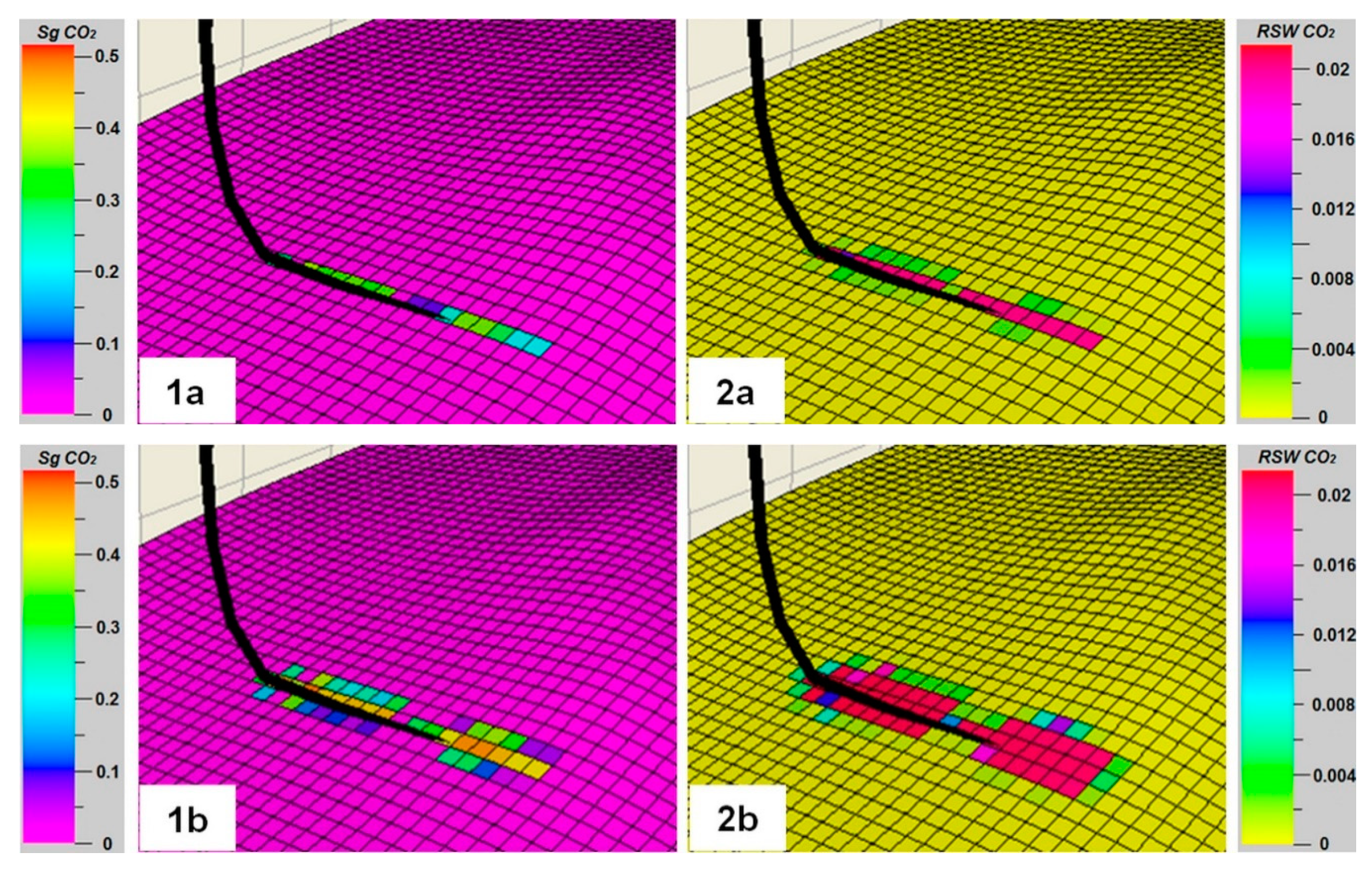
Figure 18 illustrates the saturation distribution of injected carbon dioxide in the injected layer of the Dębowiec formation in individual intervals of time. As in previous models, it is clear that the brine containing dissolved CO
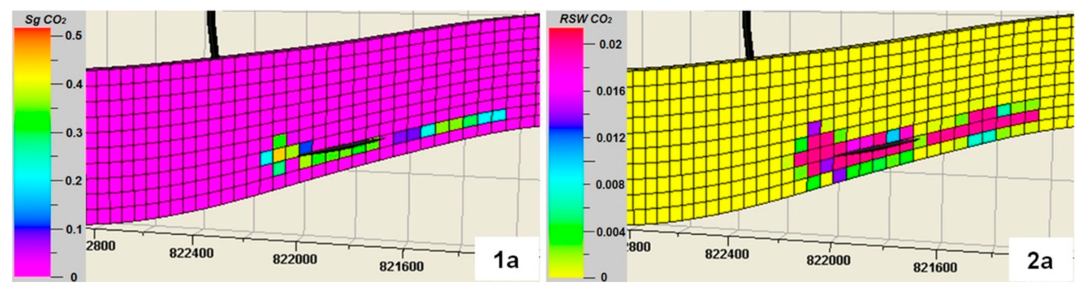
2 is spreading over a much larger area than the zone of residual CO
2. In addition, the vertical section through the injection zone (
Figure 19) shows free CO
2 saturation in the aquifer (carbon dioxide remaining in the residual state) which is presented in the form of a common fraction, while the distribution of CO
2 dissolved in the brine is presented in the form of a molar fraction for individual simulation time intervals.


