Article

Risk Assessment Method for Integrated Transmission–Distribution System Considering the Reactive Power Regulation Capability of DGs

1
School of Electrical Engineering, Southeast University, Nanjing 210096, China
2
State Grid Jiangsu Electric Co. Ltd., Nanjing 210000, China
3
National Electric Power Dispatching and Control Center, State Grid Corporation of China, Beijing 100031, China
*
Author to whom correspondence should be addressed.
Energies 2019, 12(16), 3040; https://doi.org/10.3390/en12163040
Submission received: 5 July 2019 / Revised: 31 July 2019 / Accepted: 3 August 2019 / Published: 7 August 2019
(This article belongs to the Section F: Electrical Engineering)

Abstract

:
High distributed generation (DG) penetration makes the traditional method of equalizing the distribution power system (DPS) to the PQ load bus in the risk assessment of the transmission power system (TPS) no longer applicable. This paper proposes a risk assessment method for an integrated transmission–distribution system that considers the reactive power regulation capability of the DGs. Based on the DG’s characteristics and network constraints, the regulation capacity is mapped to the boundary buses of the distribution networks. Coordinating the relationship between reactive power and active power, the utilization of the regulation capacity is maximized to reduce the load shedding in the fault analysis of the TPS. Simulation results in the integrated transmission–distribution system illustrate that the effective use of the regulation capacity of the DPS can reduce the risk of the TPS. The method can be applied to the reactive power sources planning and dispatching of power system.

1. Introduction

With the integration of a large number of DGs, the distribution network has changed from the traditional passive network to the active network with bi-directional power flow [1,2]. The influence of distribution network power flow on the reliability of transmission network continues to increase [3]. Risk assessment methods can be used to analyze the reliability of power systems [4,5,6]. Conventionally, risk assessment of transmission and distribution power systems is separated. Since the power flow in the traditional distribution network is unidirectional, the boundary buses are taken as PQ buses in the risk assessment of the TPS [7,8,9], which means its subordinate distribution networks remain unchanged, while with the increasing number of DGs, the DPS can provide power support for the TPS in emergency [2].
The supporting capacity of DPS mainly comes from the DGs. Although DGs have limited active power regulation capacity because of operating at maximum active power output state, they can provide reactive power regulation capacity through inverters. At present, research on DGs mainly focuses on the distribution network service. Efficient utilization of DGs’ reactive power regulation capability can control the voltage and minimize the network loss of the DPS [10,11,12]. In order to achieve this target, smart inverters are developed and many control strategies are studied [13]. The increasing DGs may result in some conventional power plants being shut down, and there is a shortage of reactive power source in the TPS [14]. Researchers have considered using the distribution network to provide the reactive power regulating capacity for the TPS when necessary, which has demonstrated a positive effect [15,16,17,18,19]. Ref. [15] analyzes the necessity of utilizing the reactive power potential of the DPS, and determines the potential of reactive power using optimal power flow. In [16,17], the authors propose a transmission–distribution-coupled static voltage stability assessment method, and simulations show that the reactive power support capability of the DGs can improve the voltage stability margin of the TPS. The authors of [18] present an optimization method of DPS to transform the distribution feeder into a controllable P–V bus. The work in [19] demonstrates that photovoltaic systems in the distribution network can provide reactive power regulation services to other networks. All the above studies have shown the necessity and effectiveness of using the reactive power regulation capability of the DPS.
Therefore, the characteristics of the distribution network should be considered in the risk assessment of the TPS. In [3,20], the authors propose a hierarchical risk assessment method in which, based on the assessment result of the TPS, detailed load loss calculation is analyzed in the DPS considering the impact of DGs. However, the support capability the DPS is not considered when calculating the load shedding of the TPS. Moreover, DC power flow analysis method is adopted and the impact of reactive power is not considered in the risk assessment.
When analyzing the risk of the TPS, the reactive power regulation capability needs to be fully considered in the equivalent model of distribution network with DGs. Moreover, due to the limited capacity of DG’s inverter, the active power state of DGs needs to be considered when utilizing DGs’ reactive power; thus, the active power should also be considered when modeling the supporting capacity of the DPS.
This paper proposes a risk assessment method for integrated an transmission–distribution system that considers the reactive power regulation capability of the DGs. Considering the DG’s characteristics and network constraints, the DG’s reactive power regulation capability is mapped to the boundary bus as the reactive power potential of the DPS. The reactive power regulation capability of the DPS is considered when assessing the operational risk of the transmission network. If the reactive power demand problem of the TPS is serious, the DG’s active power and reactive power is coordinated to further improve the reactive power regulation capacity of the DPS. The main contribution of this paper can be summarized as follows: (1) the reactive power regulation of the DPS is considered in the risk assessment of the TPS and (2) DG’s active power and reactive power is coordinated when necessary to further enhance reactive power support to the TPS.
The rest of this paper is organized as follows. In Section 2, the influence of DPS’s reactive power on TPS is analyzed. Section 3 provides the computing methods of the reactive power regulation capability of the DPS with DGs integrated. In Section 4, the risk assessment method of the TPS considering the reactive power support of the DPS is proposed. Section 5 provides the simulations of different scenarios and illustrates the results. Finally, the conclusions are presented in Section 6.

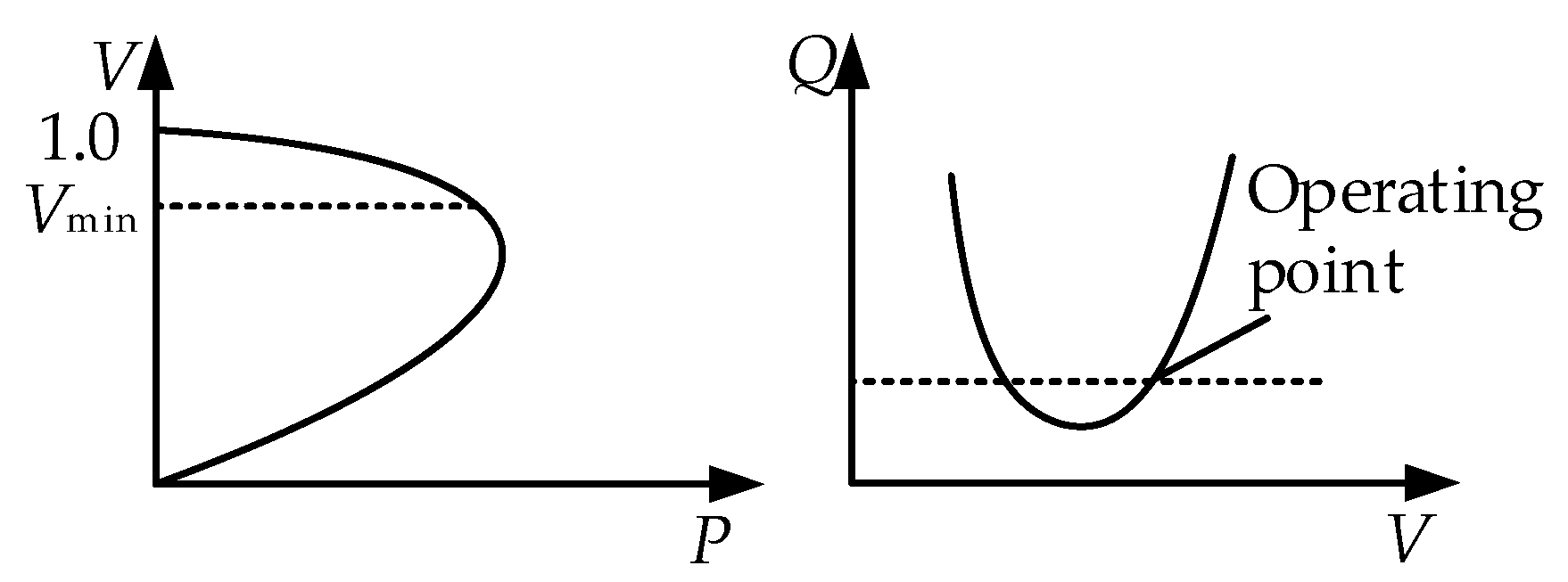
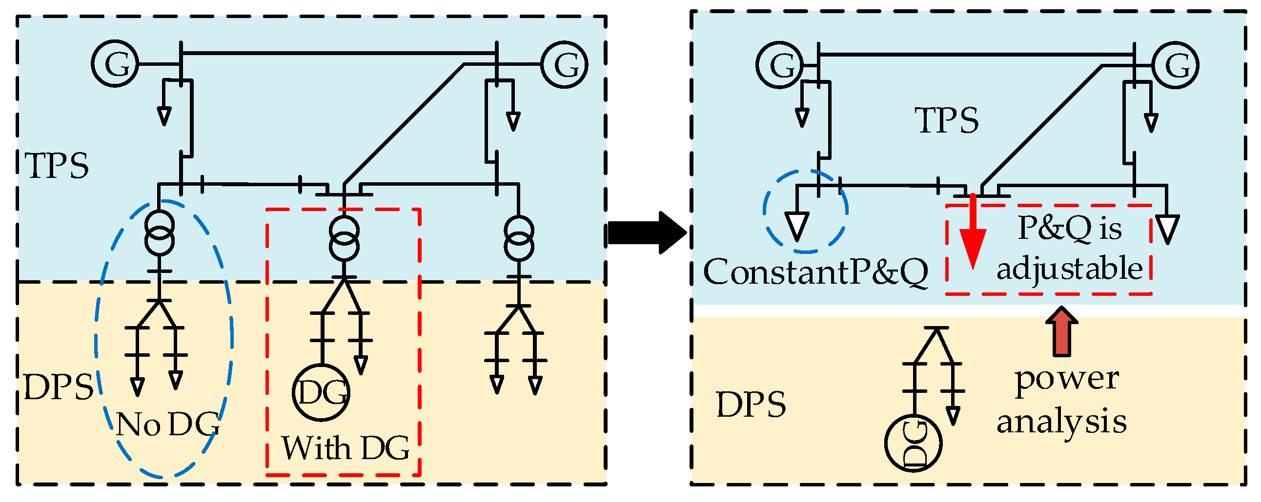
2. Influence of DPS’s Reactive Power on TPS

Figure 1 shows the relationship between active power and voltage, and the relationship between reactive power and voltage of a bus.
When a system failure occurs, the bus voltage may exceed the critical value. As can be seen from the P–V curve, appropriate load shedding can restore the voltage to the normal range. Increasing the reactive power injection of the node can also restore the voltage due to the V–Q characteristics of the bus. Therefore, from the perspective of system reliability, sufficient reactive reserve can avoid system removal load under certain circumstances and improve the reliability of power system.
The DGs connected to the distribution network have reactive output capability, which can be used to support the operation of the TPS. In the traditional risk assessment of TPS, the DPS is equivalent to a constant power load. When failure occurs in the transmission network, the reactive power regulation capability of the DGs cannot be effectively utilized in the state analysis of TPS. In this paper, the reactive power regulation capability of the DGs is mapped to the boundary bus and the resulting active power changes are considered, as shown in Figure 2. The reactive power regulation capacity is considered for power generation scheduling and load reduction calculation if failure occurs in the TPS.

3. Analysis of Reactive Power Regulation Capability of DPS with DG Integrated

Sufficient reactive power reserve can improve the reliability of the TPS. Taking distributed photovoltaic (PV) as an example, this paper analyzes the reactive power support capacity of DGs for the transmission network and maps the reactive power regulation capacity of DG to the boundary bus.

3.1. The Reactive Power Output Capacity of Distributed PV

Distributed PV is connected to the power grid through the inverter, and the relationship between its reactive power capacity and the inverter capacity can be calculated as follows:
Q P V max = S I N V 2 P P V 2
where Q P V max is the maximum reactive power output of the PV, P P V is the active power output of the PV, and S I N V is the inverter capacity of the PV.
Figure 3 shows the relationship between reactive power capacity and active power output of PV. At point a, the PV outputs active power and a certain amount of reactive power. If the reactive power demand of system is bigger, the PV’s working point move from a to b, and inverter of PV operates in the rated state. If the system still has reactive power shortage, the active output of the PV can be appropriately reduced to improve the reactive output capability, as shown by point c in the Figure 3. Moreover, the reactive power output of the inverters is not only related to the inverter’s parameters and the active power output but is also limited by the network voltage. These factors should be considered in the analysis.

3.2. Calculation of Reactive Power Regulation Capability of DPS

The flow of reactive power in the network will increase the loss of active power. When the DPS operates in the state of minimum loss of active power, providing reactive power support to the upstream network will increase the network loss. The active power of DPS obtained from the TPS will be increased. In Figure 4, the abscissa Δ Q indicates the reactive power changes and the ordinate Δ P indicates the active power changes obtained by the DPS obtains from the TPS. The red curve indicates the relationship between reactive power change and active power change that the DPS obtains from the TPS when PVs operate in the state of maximum output of active power. In this stage, the reactive power of PVs is adjusted within the inverter capacity range with the active power output kept constant. The active power is only affected by the change of the reactive power. Due to the limited capacity of the inverter, when the problem of the reactive power demand of the TPS is serious, it is difficult for the remaining reactive power capacity of the PV that operates in the state of maximum active power output is difficult the reactive power requirements of the system. Active power reduction is required for some PVs to release reactive capacity. In this stage, the relationship between the change of reactive power and the change of active power that the DPS obtains from the TPS is shown as the blue curve in Figure 4. The factors that affect the active power include the network loss and the active reduction of the PV.
The relationship between Δ P and Δ Q can be expressed as follows:
f ( Δ Q ) Δ P = 0
In order to obtain the relationship between Δ P and Δ Q in Figure 4, the linearization method is used in the calculation process, as shown by the purple line in the figure. There will be some error between the linearized curve and the actual curve, as shown by the yellow area. If the curve is linearized in multiple stages so that the Δ Q 1 is small enough, the error caused by linearization is very small and can be neglected, as shown by the Δ Q 2 and the Δ Q 3 in Figure 4. When PVs work in the maximum active power output state, Δ P varies very little with Δ Q and their relationship can be approximated as linear, as shown in Section 3.2.1. However, in the stage of PVs’ operating with active power reduction, Δ P varies greatly with Δ Q , and small-step multi-stage linearization is required to perform, as shown in Section 3.2.2.

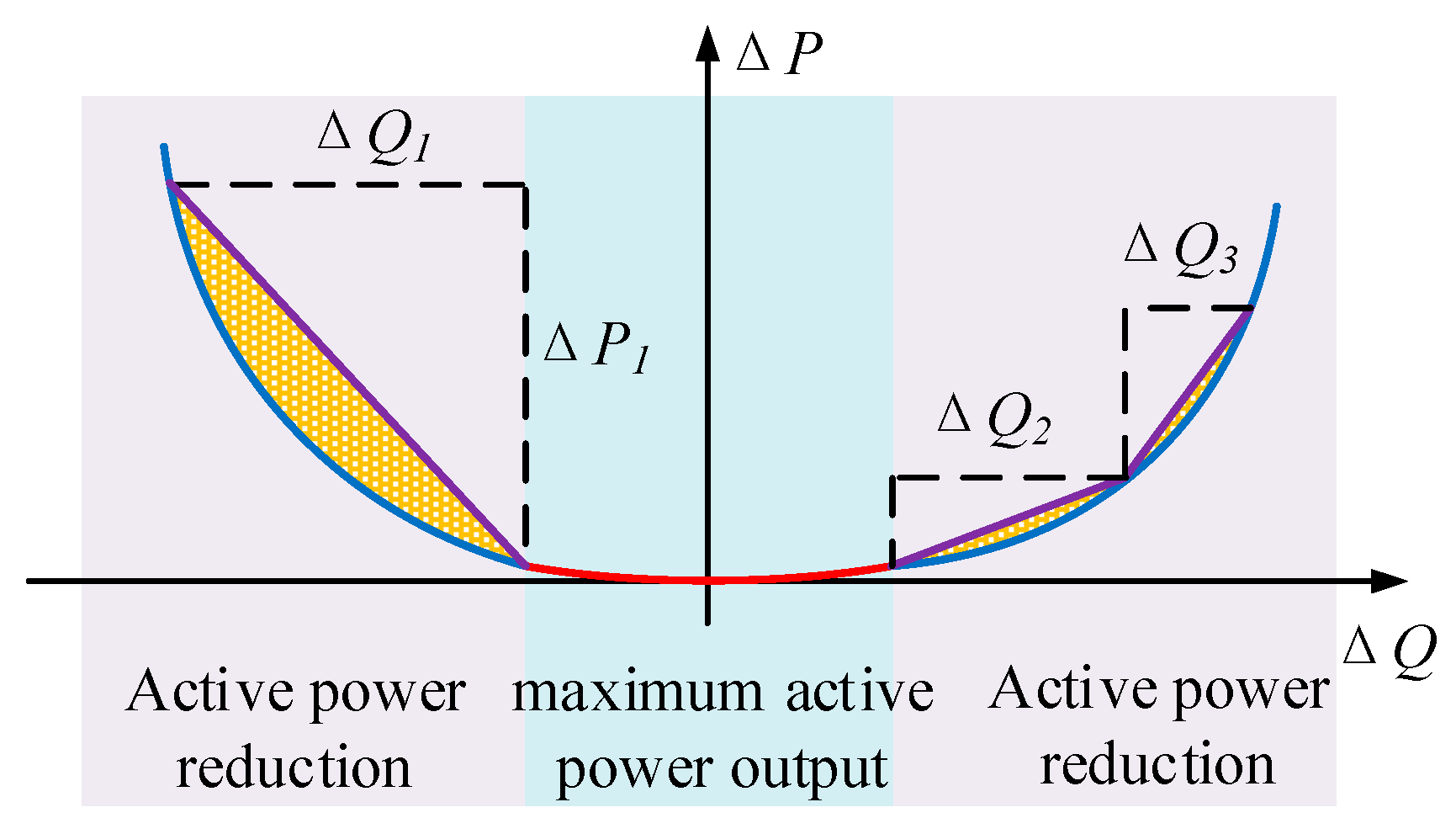
3.2.1. Maximum Active Power Output State

The reactive power output of PVs is not only limited by the inverter capacity, but also by the feeder voltage. When the PVs are at the maximum active power output state, the reactive power support capability that the DPS can provide can be calculated by Equations (3) and (4). Equation (3) shows the minimum value of the inductive reactive power that DPS obtains from the TPS, that is, the maximum value of inductive reactive power that the DPS can provide to the TPS. Equation (4) shows the maximum value of capacitive reactive power that the DPS can provide to the TPS.
{ Δ Q 0 = min ( Q D Q D 0 ) Δ P 0 = P D P D 0 k 0 = Δ P 0 / Δ Q 0
{ Δ Q 0 + = max ( Q D Q D 0 ) Δ P 0 + = P D P D 0 k 0 + = Δ P 0 + / Δ Q 0 +
where Δ Q 0 and Δ Q 0 + are the maximum value of inductive reactive power and capacitive reactive power that the DPS can provide to the TPS based on the initial state, respectively; Δ P 0 and Δ P 0 + are the increase in active power demand of the DPS corresponding to Δ Q 0 and Δ Q 0 + , respectively; k 0 and k 0 + are the linear relationship coefficients of Δ P and Δ Q when DPS provides inductive reactive power and capacitive reactive power, respectively; Q D and P D are the value of the inductive reactive power and active power obtained by the DPS from the TPS, respectively; and Q D 0 , P D 0 are the value of initial state, respectively.
For the model presented in Equations (3) and (4), the corresponding constraints include power equation, DGs constraints, and security constraints, which are formulated as follows:
{ P G i P L i V i j Ω V j ( G i j cos δ i j + B i j sin δ i j ) = 0 Q G i Q L i V i j Ω V j ( G i j sin δ i j B i j cos δ i j ) = 0 V i min V i V i max π δ i j π P D G i = P D G i max ( P D G i max ) 2 + ( Q D G i max ) 2 = ( S D G i ) 2 | Q D G i | Q D G i max
where P G i and Q G i are the active and reactive power of the power source of node I, respectively, and the power source are mainly DGs in DPS; P L i and Q L i are the active and reactive power of the load, respectively; G i j and B i j are the admittance matrix elements of the network, respectively; δ i j is the voltage phase angle difference; V i is the voltage of node i; V i min and V i max are the lower and upper limits on the voltage of node I, respectively; P D G i and Q D G i are the active and reactive power output of the PV at node I, respectively; P D G i max and Q D G i max are the maximum value of active and reactive power of PV at node I, respectively; and S D G i is the inverter capacity of the PV at node i.
According to the above model, the red curve part in Figure 4 can be obtained, that is, the function relationship between Δ P and Δ Q when PVs operate in the state of maximum output of active power.

3.2.2. Active Power Reduction State

When the problem of the reactive power demand of the TPS is serious, active power reduction is required for some PVs to release reactive capacity. In this stage, Δ P varies greatly with Δ Q . To obtain the function relationship between Δ P and Δ Q , the value of Δ P can be fixed by multiple stages, and the corresponding Δ Q can be calculated in the process. The mathematic model of this stage can be described as follows:
{ Q D n = Q D n 1 + Δ Q 1 Δ P n = min P D n P D n 1 k n = Δ P n / Δ Q 1
where Δ Q 1 is the step size of reactive power change; Q D n is the reactive power obtained by DPS from the TPS in the step n, P D n is the active power obtained by DPS from the TPS in the step n corresponding to Q D n , Δ P n is change of the active power obtained by DPS from the TPS in the step n, and k n is the linear relationship coefficients of Δ P and Δ Q in the step n.
Constraints in active power reduction state model consist of power equation, DGs constraints, and security constraints, just like the Equations (5). The constraint on the DGs active power output needs to be changed as follows:
0 P D G i P D G i max
The Equation (7) allows PVs to perform active power reduction to release reactive capacity. According to the above model, the blue curve part in Figure 4 can be obtained, that is, the function relationship between Δ P and Δ Q when PVs operate in the state of active power reduction.

4. Risk Assessment Method of TPS Considering the Reactive Power Support of DPS

In the risk assessment of the TPS, the state of the system is first simulated, and then each state is analyzed to determine whether there are system problems and calculate the consequences of the system problems. The Monte Carlo simulation method is used to sample the system generators and lines to simulate the system status in this paper [21]. For all generators and power transmission and transformation components in the system, two states model are used for simulation.

4.1. System State Analysis

After selecting the system state, the fault analysis of the system is carried out and the power generation is rescheduled to eliminate the off-limit of the system. If the load shedding cannot be avoided, the reactive power support of the DPS needs to be considered to calculate the load shedding. The AC optimal power flow is used to adjust the generator output and load shedding. The objective is formulated as follows:
C = min i = N ( P T L i P t l i )
where P T L i is the active power of node i in the transmission network before load shedding, P t l i is the active power of node i in the transmission network after load shedding, and N is the number of nodes in transmission network.
Constraints consist power equations, generators output constraints, load power constraints, reactive power support of DPS constraints, and network security constraints:
{ P G i P t l i Δ P d i V i j Ω V j ( G i j cos δ i j + B i j sin δ i j ) = 0 Q G i Q t l i Δ Q d i V i j Ω V j ( G i j sin δ i j B i j cos δ i j ) = 0 P G i min P G i P G i max , Q G i min Q G i Q G i max 0 P t l i P T L i , 0 Q t l i Q T L i Δ Q d i min Δ Q d i Δ Q d i max , f ( Δ Q d i ) Δ P d i = 0 V i min V i V i max , π δ i j π , T k ( V , δ ) T k max
where Q t l i is the reactive power of node i in the transmission network after load shedding; Δ P d i and Δ Q d i are the reactive power change and the corresponding active power change of the DPS connected to the bus i of the transmission network, respectively; P G i min and P G i max are the maximum and minimum active power output of generators at node i, respectively; Q G i min and Q G i max are the maximum and minimum reactive power output of generators at node i, respectively; Δ Q d i min and Δ Q d i max are the maximum value of inductive reactive power and capacitive reactive power that the DPS can provide to the TPS, respectively; and T k and T k max are the power flow and the power flow limit of line k, respectively.
After calculating the load shedding and the reactive power provided by the DPS, the active power P D and reactive power Q D of the boundary bus can be obtained. If there is load shedding, it is necessary to further determine whether the DPS can meet the active and reactive power state requirements of the boundary bus. The method of fixed active power and optimized reactive power is used to distinguish the following:
{ P D = P D min f = ( Q D Q D ) 2
Constraints consist of power equation, DGs constraints, and security constraints. Load shedding is allowed during optimization. If min f ε ( ε is a small number), it can be considered that the DPS can meet the boundary bus power state requirements. Otherwise, the optimized reactive power error is sent to the TPS to further optimize the load reduction.

4.2. Risk Indicator

The risk indicator considers the probability and consequences of the event. According to the risk theory, this paper uses the risk of loss of load to characterize the system.

4.2.1. Loss of Load Probability

Loss of load probability (LOLP) is the probability that the power system cannot meet the demand of load. The calculation method of this indicator can be expressed as follows:
L O L P = 1 S k = 1 S F k
where S is the total number of system samples and F k is the indicative variable of the system load shedding in the sampling k.
F k = { 0 , no   load   shedding ; 1 , load   shedding

4.2.2. Expected Power Not Served

Expected power not served (EPNS) represents the expected value of the total amount of power lost by the system due to the load shedding event. The calculation method can be expressed as follows:
E P N S = 1 S k = 1 S D k
where Dk is the total system load shedding in the sampling k.

4.3. Steps of Risk Assessment

The calculation steps for the risk assessment method of TPS considering the reactive power support of DPS are as follows:
(1)
The power flow analysis is utilized in the DPS to obtain the relationship between Δ P and Δ Q of the DPS;
(2)
Monte Carlo simulation method is used to simulate the system status. For all generators and power transmission and transformation components in the system, two states model are used for simulation;
(3)
The fault analysis of the TPS is carried out, and the power generation is rescheduled to eliminate the off-limit of the system. If the load shedding cannot be avoided, the reactive power support of the DPS needs to be considered to calculate the load shedding;
(4)
According to the load shedding and the reactive power provided by the DPS, calculate the active and reactive power of the boundary bus. Determine whether the DPS can meet the active and reactive power state requirements of the boundary bus. If the error of reactive power exceeds the limit, send the error to the TPS to further optimize the load reduction;
(5)
If the number of samples reaches the given maximum number, the calculation is terminated; otherwise, return to step (2) for the next sampling;
(6)
Calculate risk indicators LOLP and EPNS.

5. Case Study

This section presents case study based on the integrated transmission–distribution system shown in the Figure 5. The transmission system is IEEE RTS [22], and the load of buses 3, 9, 10, 14, and 19 is extended into multiple distribution systems, as shown in Figure 5. The distribution system adopts modified IEEE 33-bus system. In the simulation, 20 IEEE 33-bus systems are connected to the bus that is expanded into the distribution network. The parameters of the distribution network are modified, as shown in the Table 1. There are thirteen 1.0-MVA PVs in the distribution network, and their maximum active power is 0.8 MW. The load in the distribution network is modified so that the load of the transmission network at 12pm is consistent with the initial RTS system. The proportion of load connected to each bus in the 33-bus system is shown in the Table 2.

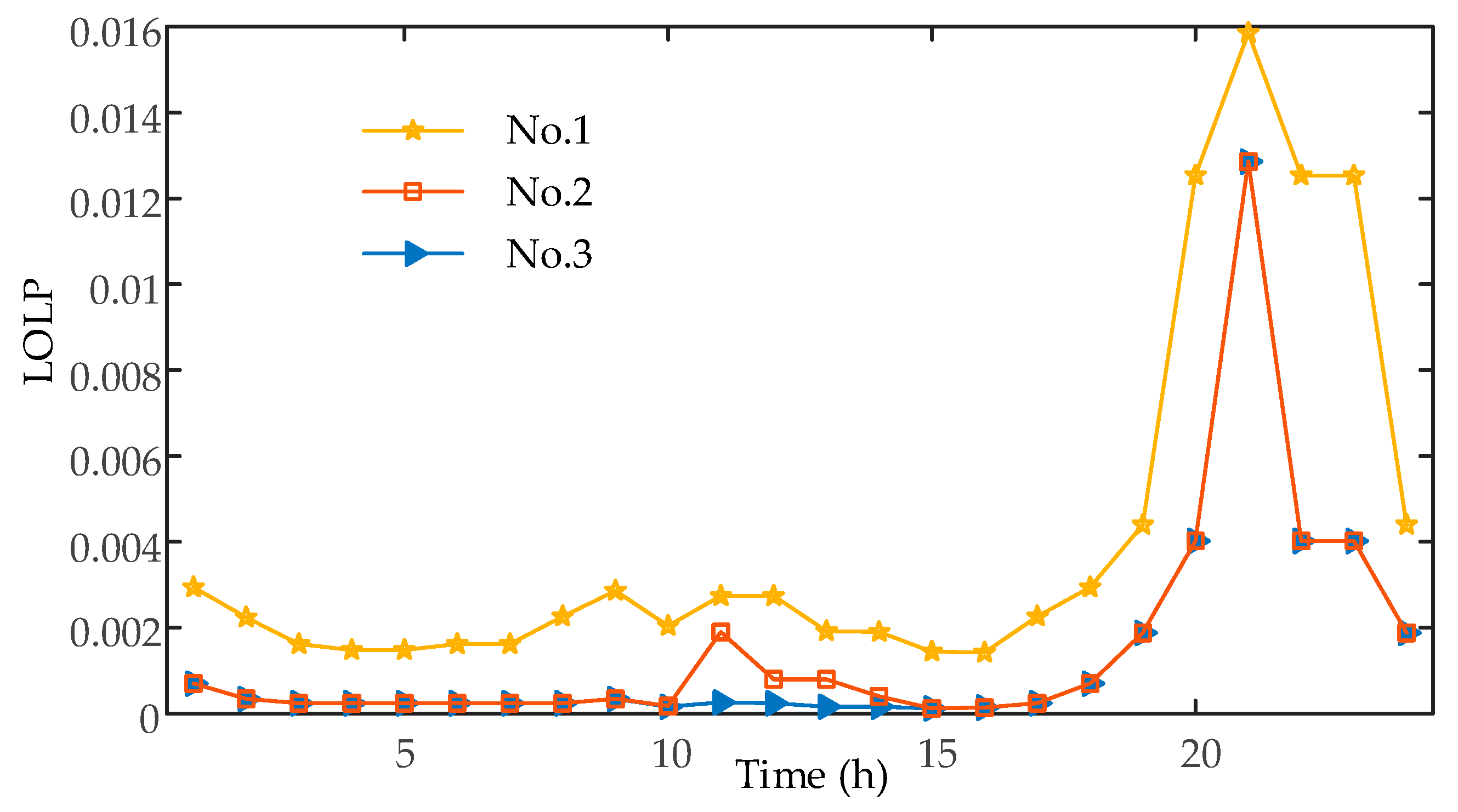
5.1. Risk Assessment of TPS

In the each DPS, the initial state of distributed PV is outputting all the active power and outputting some reactive power to minimize the network loss of the DPS. The system’s 24-h operational risks are analyzed. Figure 6 shows the load curve and the distributed PV active power curve of the system.
When failure occurs and load shedding is unavoidable, all loads are considered to be equally important. The following four methods are used to calculate the risk indicators of the system:
(1)
The reactive power regulation capacity of the DPS is not considered;
(2)
Consider the reactive power regulation capacity of the DPS, but do not consider the active power reduction of DGs;
(3)
Consider the reactive power regulation capacity of the DPS, and consider the active power reduction of DGs.
Figure 7 and Figure 8 show the system’s 24-h risk indicators LOLP and EPNS, respectively. Compared with not considering the reactive power support capacity of the DPS, the effective use of the reactive power regulation capacity of the DPS can reduce the risk of the TPS. At noon, the active power output of PVs is large and the reactive power adjustment capability provided by the DPS is small. Proper reduction of the active power of the PVs can release more reactive power capacity to support the TPS. The risk indicators LOLP and EPNS are both smaller in 11 h after considering the active power reduction of distributed PVs. In the evening and at night, PVs have large reactive output capability because they do not output active power, and the DPS has a greater range of reactive power adjustment. The load reaches a peak during the 19–23 h period, which is more likely to cause overload and out-of-voltage limit problems. The effect of utilizing the reactive power regulation capability of the DPS to reduce the operational risk of the upstream network is more significant during this period.

5.2. Analysis of Factors Affecting PV Active Power Reduction

Based on the load and the PV data at 11h, the other factors are kept constant, and the line transmission power limit of the TPS is changed. The line transmission power limit is set to be α times of the initial value, taking α as 0.8, 0.9, and 1.0, respectively. The DG active power reduction probability (DGAPRP) and DG active power reduction expectation (DGAPRE) are used to characterize the degree of active power reduction of DG. The calculation method of the two indicators is shown in Equation (14). The LOLP, EPNS, DGAPRP, and DGAPRE of the system are shown in Table 3.
{ D G A P R P = 1 S k = 1 S E k E k = { 0 no   DG   active   power   reduction 1 DG   active   power   reduction D G A P R E = 1 S k = 1 S M k
where E k is the indicative variable of the system with DG active power reduction in the sampling k and M k is the total active power reduction of DG in the sampling k.
The line transmission power limit is kept constant as 0.9 times of the initial value, and the capacity of the grid-connected inverter of DGs is changed so that the active power value of DG is β times of the inverter capacity. Taking β as 0.85, 0.9, and 0.95, respectively, the LOLP, EPNS, DGAPRP, and DGAPRE of the system are shown in Table 4.
It can be seen from Table 3 and Table 4 that increasing the transmission power limit of the line or increasing the capacity of the DG grid-connected inverter can not only reduce the risk of the TPS, but also reduce the active power reduction of the DGs in the DPS. The active power reduction of DGs is a measure taken to release more reactive power capacity when the reactive power demand problem of the TPS is serious and the reactive power output capability DGs is small. When the transmission power of the transmission line reaches the limit, it is necessary to minimize the transmission of reactive power in the line to increase the margin of active power transmission. Increasing the line capacity also increases the margin of active power transmission, so it can alleviate the problem of reactive power demand of the system. Increasing the capacity of the grid-connected inverter directly increases the reactive output capability of the DGs. Therefore, changing these two factors can affect the risk of the TPS and the active power reduction of the DGs in the DPS.

5.3. Influence of DGs’ Location on TPS Risk

Based on the load and the PV data at 11 h, the other factors are kept constant, and the location of the PVs in the DPS is changed, as shown in Table 5. The normalized calculation results of the system risk indicators in the three cases are shown in Figure 9.
It can be seen from Figure 9 that when the distribution of DGs is more scattered in the DPS, the risk value of the TPS is smaller. The reason is that when DGs are connected to the DPS in a more concentrated form, it may cause the voltage to exceed the limit. Thus, the reactive power output range of the DGs may be reduced due to the voltage limit of the DPS, and the DPS can provide smaller reactive power support capability for the TPS. So, it is reasonable, as shown in Figure 9, that the risk value of case 3 is larger.

6. Conclusions

This paper proposes a risk assessment method for the integrated transmission–distribution system. DG’s active power and reactive power is coordinated to calculate the reactive power potential of the DPS, which is utilized to reduce the amount of load shedding in the failure analysis when performing risk assessment of the TPS. From the simulation results, the effect of utilizing the reactive power regulation capability of the DPS to reduce the operational risk of the TPS is more significant during peak load period. The risk assessment method takes into account the reactive power regulation potential of the DPS, and can be applied to the reactive power sources planning and operation mode adjustment of the transmission network, while the proposed method is based on the interaction of transmission system operator (TSO) and distribution system operator (DSO). Related policies and economic considerations remain to be studied.

Author Contributions

Q.W., D.S., J.H., and Y.T. contributed in developing the ideas of this research. Q.W., D.S., and J.H. performed this research. All the authors read and approved the final manuscript.

Funding

This research was funded by State Grid Corporation Project of China “Key technology research and demonstration application of transmission–distribution integrated system with distributed operation and centralized analysis”.

Conflicts of Interest

The authors declare no conflict of interest.

References

  1. Lin, C.; Wu, W.; Zhang, B.; Wang, B.; Zheng, W.; Li, Z. Decentralized Reactive Power Optimization Method for Transmission and Distribution Networks Accommodating Large-Scale DG Integration. IEEE Trans. Sustain. Energy 2017, 8, 363–373. [Google Scholar] [CrossRef]
  2. Jain, H.; Rahimi, K.; Tbaileh, A.; Broadwater, R.P.; Jain, A.K.; Dilek, M. Integrated transmission & distribution system modeling and analysis: Need & advantages. In Proceedings of the IEEE Power and Energy Society General Meeting, Boston, MA, USA, 17–21 July 2016; pp. 1–5. [Google Scholar]
  3. Jia, H.; Qi, W.; Liu, Z.; Wang, B.; Zeng, Y.; Xu, T. Hierarchical risk assessment of transmission system considering the influence of active distribution network. IEEE Trans. Power Syst. 2015, 30, 1084–1093. [Google Scholar] [CrossRef]
  4. Liang, C.; Wang, P.; Han, X.; Qin, W.; Billinton, R.; Li, W. Operational Reliability and Economics of Power Systems with Considering Frequency Control Processes. IEEE Trans. Power Syst. 2017, 32, 2570–2580. [Google Scholar] [CrossRef]
  5. Ansari, O.A.; Chung, C.Y. A hybrid framework for short-term risk assessment of wind-integrated composite power systems. IEEE Trans. Power Syst. 2019, 34, 2334–2344. [Google Scholar] [CrossRef]
  6. Deng, W.; Zhang, B.; Ding, H.; Li, H. Risk-based probabilistic voltage stability assessment in uncertain power system. Energies 2017, 10, 180. [Google Scholar] [CrossRef]
  7. Lin, W.M.; Yang, C.Y.; Tu, C.S.; Tsai, M.T. An optimal scheduling dispatch of a microgrid under risk assessment. Energies 2018, 11, 1423. [Google Scholar] [CrossRef]
  8. Shahidehpour, M.; Li, Z.; Liu, X.; Li, Z.; Cao, Y.; Liu, X. Power System Risk Assessment in Cyber Attacks Considering the Role of Protection Systems. IEEE Trans. Smart Grid 2016, 8, 572–580. [Google Scholar]
  9. Yong, P.; Zhang, N.; Kang, C.; Xia, Q.; Lu, D. MPLP-Based Fast Power System Reliability Evaluation Using Transmission Line Status Dictionary. IEEE Trans. Power Syst. 2019, 34, 1630–1640. [Google Scholar] [CrossRef]
  10. Zhang, L.; Tang, W.; Liang, J.; Cong, P.; Cai, Y. Coordinated Day-Ahead Reactive Power Dispatch in Distribution Network Based on Real Power Forecast Errors. IEEE Trans. Power Syst. 2016, 31, 2472–2480. [Google Scholar] [CrossRef]
  11. Onlam, A.; Yodphet, D.; Chatthaworn, R.; Surawanitkun, C.; Siritaratiwat, A.; Khunkitti, P. Power Loss Minimization and Voltage Stability Improvement in Electrical Distribution System via Network Reconfiguration and Distributed Generation Placement Using Novel Adaptive Shuffled Frogs Leaping Algorithm. Energies 2019, 12, 553. [Google Scholar] [CrossRef]
  12. Chen, Q.; Zhao, X.; Gan, D. Active-reactive scheduling of active distribution system considering interactive load and battery storage. Prot. Control Mod. Power Syst. 2017, 2, 29. [Google Scholar] [CrossRef] [Green Version]
  13. Ustun, T.S.; Aoto, Y. Analysis of smart inverter’s impact on the distribution network operation. IEEE Access 2019, 7, 9790–9804. [Google Scholar] [CrossRef]
  14. Li, Z.; Wang, J.; Sun, H.; Qiu, F.; Guo, Q. Robust Estimation of Reactive Power for an Active Distribution System. IEEE Trans. Power Syst. 2019. [Google Scholar] [CrossRef]
  15. Goergens, P.; Potratz, F.; Godde, M.; Schnettler, A. Determination of the potential to provide reactive power from distribution grids to the transmission grid using optimal power flow. In Proceedings of the Universities Power Engineering Conference, Stoke on Trent, UK, 1–4 September 2015. [Google Scholar]
  16. Li, Z.; Guo, Q.; Sun, H.; Wang, J. Impact of Coupled Transmission–distribution on Static Voltage Stability Assessment. IEEE Trans. Power Syst. 2017, 32, 3311–3312. [Google Scholar] [CrossRef]
  17. Li, Z.; Guo, Q.; Sun, H.; Wang, J.; Xu, Y.; Fan, M. A Distributed Transmission–distribution-Coupled Static Voltage Stability Assessment Method Considering Distributed Generation. IEEE Trans. Power Syst. 2018, 33, 2621–2632. [Google Scholar] [CrossRef]
  18. Arnold, D.B.; Sankur, M.D.; Negrete-Pincetic, M.; Callaway, D.S. Model-free optimal coordination of distributed energy resources for provisioning transmission-level services. IEEE Trans. Power Syst. 2018, 33, 817–828. [Google Scholar] [CrossRef]
  19. Valverde, G.; Shchetinin, D.; Hug-Glanzmann, G. Coordination of Distributed Reactive Power Sources for Voltage Support of Transmission Networks. IEEE Trans. Sustain. Energy 2019, 10, 1544–1553. [Google Scholar] [CrossRef]
  20. Xu, C.; Sun, D.; Tang, Y.; Yu, J.; Wu, H. Risk Assessment Method for Transmission–distribution Integrated System with Distributed PV. In Proceedings of the 2018 2nd IEEE Conference on Energy Internet and Energy System Integration, Beijing, China, 20–22 October 2018; pp. 1–6. [Google Scholar]
  21. Li, W.; Zhou, J.; Xie, K.; Xiong, X. Power system risk assessment using a hybrid method of fuzzy set and Monte Carlo simulation. IEEE Trans. Power Syst. 2008, 23, 336–343. [Google Scholar]
  22. Subcommittee, P.M. IEEE reliability test system. IEEE Trans. Power Appar. Syst. 1979, 6, 2047–2054. [Google Scholar] [CrossRef]
Figure 1. Power-voltage (P–V) and voltage-reactive power (V–Q) curve of bus.
Energies 12 03040 g001
Figure 2. Diagram of transmission power system (TPS) analysis considering reactive power regulation of distribution power system (DPS).
Energies 12 03040 g002
Figure 3. The relationship between reactive power capacity and active power output of PV.
Energies 12 03040 g003
Figure 4. Schematic diagram of the curve showing the relationship of reactive power and active power change that the DPS obtained from the TPS.
Energies 12 03040 g004
Figure 5. The integrated transmission–distribution system.
Energies 12 03040 g005
Figure 6. The load curve and the distributed PV active power curve.
Energies 12 03040 g006
Figure 7. Curves of risk indicator loss of load probability (LOLP).
Energies 12 03040 g007
Figure 8. Curves of risk indicator expected power not served (EPNS).
Energies 12 03040 g008
Figure 9. System risk under different DGs’ location.
Energies 12 03040 g009
Table 1. Modified 33-bus system branch parameter (p.u.).
BranchrxBranchrxBranchrxBranchrx
1-20.0190.0209-100.2170.30817-180.1520.2396-260.0420.043
2-30.1030.10410-110.0410.0272-190.0340.06526-270.0590.060
3-40.0760.07811-120.0780.05119-200.3130.56427-280.2200.388
4-50.0790.08112-130.3050.48020-210.0850.19928-290.1670.291
5-60.1700.29413-140.1130.29721-220.1470.39029-300.1060.108
6-70.0390.25714-150.1230.2193-230.0940.12830-310.2030.401
7-80.1480.09815-160.1550.22723-240.1870.29531-320.0650.151
8-90.2140.30816-170.2680.71624-250.1860.29232-330.0710.221
Table 2. Proportion of each bus load in the 33-bus system.
BusPQBusPQBusPQBusPQ
20.0270.032100.0160.008180.0240.015260.0160.009
30.0240.015110.0120.011190.0240.015270.0160.009
40.0320.030120.0160.013200.0240.015280.0160.008
50.0160.011130.0160.013210.0240.226290.0320.026
60.0160.008140.0320.030220.0240.015300.0540.023
70.0540.038150.0160.004230.0240.019310.0400.026
80.0540.038160.0160.008240.1130.226320.0570.004
90.0160.008170.0160.008250.1130.075330.0160.015
Table 3. Risk and DG active power reduction under different line transmission power limits.
αLOLPEPNSDGAPRPDGAPRE
0.80.011320.289600.038730.38251
0.90.005320.178500.023160.12184
1.00.000280.123260.014800.05507
Table 4. Risk and DG active power reduction under different grid-connected inverter capacities.
βLOLPEPNSDGAPRPDGAPRE
0.850.005130.173310.000470.00628
0.90.005230.177170.008400.03552
0.950.005320.178500.023160.12184
Table 5. PVs’ location.
CasesBus in the DPS with PVs Connected
Case 16, 8, 11, 13, 16, 18, 20, 22, 23, 25, 29, 31, 33
Case 211(3) 1, 18(3), 22(2), 25(2), 33(3)
Case 318(5), 25(3), 33(5)
1 The number in brackets are the number of PVs connected to the bus.

