Thermodynamic Evaluation of LiCl-H₂O and LiBr-H₂O Absorption Refrigeration Systems Based on a Novel Model and Algorithm

Abstract

An absorption refrigeration system (ARS) is an alternative to the conventional mechanical compression system for cold production. This study developed a novel calculation model using the Matlab language for the thermodynamic analysis of ARS. It was found to be reliable in LiCl-H₂O and LiBr-H₂O ARS simulations and the parametric study was performed in detail. Moreover, two 50 kW water-cooled single effect absorption chillers were simply designed to analyze their off-design behaviors. The results indicate that LiCl-H₂O ARS had a higher coefficient of performance (COP) and exergetic efficiency, particularly in the lower generator or higher condenser temperature conditions, but it operated more restrictively due to crystallization. The off-design analyses revealed that the preponderant performance of LiCl-H₂O ARS was mainly due to its better solution properties because the temperature of each component was almost the same for both chillers in the operation. The optimum inlet temperature of hot water for LiCl-H₂O (83 °C) was lower than that of LiBr-H₂O (98 °C). The cooling water inlet temperature should be controlled within 41 °C, otherwise the performances are discounted heavily. The COP and cooling capacity could be improved by increasing the temperature of hot water or chilled water properly, contrary to the exergetic efficiency.

1. Introduction

As a promising technology to use low thermal potential energy and renewable energy, an absorption refrigeration system (ARS) is getting significant attention nowadays because it can be driven by waste heat [1], biomass [2], solar [3], geothermal energy [4], etc., instead of conventional compression-work-driven chillers. Furthermore, the ARS typically uses water as a refrigerant and the working fluids of system operation are environmentally friendly with zero global warming potential (GWP) and ozone depletion potential (ODP) [5].

In the ARS, the type of absorbent–refrigerant pair selected plays a major role in the performance. Sun et al. [6] has presented a complete review of working pairs of absorption cycles by dividing them into five general series according to the kinds of refrigerant. However, there are limited pairs commercially available from very large to small capacities. Among them, the most commonly used pairs are lithium bromide-water (LiBr-H₂O) for a higher coefficient of performance (COP) and aqua ammonia (H₂O-NH₃) for producing cold at a lower temperature level [7]. A H₂O-NH₃ ARS is more complicated as it requires a rectifier mechanism to separate water vapor from ammonia, whereas the main problem for LiBr-H₂O ARS is the crystallization, which is also present for other salt-based aqueous solutions [8]. In recent years, numerous analyses have been undertaken to find better alternative working pairs of ARS, mostly using H₂O and NH₃ as refrigerants [9,10,11,12]. According to these studies, LiCl-H₂O seems to be one of the satisfying options as an absorption cycle working fluid for its advantages regarding the triple state point, long-term stability, comparatively lower cost, and better cycle performance, compared to LiBr-H₂O [13].

Numerous experimental studies on the properties of LiBr-H₂O and LiCl-H₂O solutions have been conducted and empirical formulations with reasonable accuracy are developed through curve fitting of the experimental data [14,15,16,17,18], which are helpful for researchers carrying out theoretical analyses of ARS using these working fluids. However, most of the studies focus on the evaluation of the LiBr-H₂O working pair and few studies are available on the analysis of LiCl-H₂O ARS. Parham et al. [19] stated that an absorption chiller using LiCl-H₂O has a ≈5–6% higher exergetic efficiency when the condensation temperature is 40 °C and absorber temperature is 35 °C, but a LiBr-H₂O working pair has a ≈0.6–0.8% higher COP under the same working conditions and even a ≈1.5–2% greater COP under the optimum conditions. Patel et al. [20] theoretically investigated a 1 RT (United States refrigeration ton) single effect LiCl-H₂O ARS on the basis of the first and second law of thermodynamics, and found that the COP of a LiCl-H₂O system is ≈4–9% higher, while the exergetic efficiency is ≈3–6% higher than that of LiBr-H₂O. Bellos et al. [21] parametrically examined the performance of a solar absorption cooling system under various heat sources and three ambient temperature levels and proved that the usage of the LiCl-H₂O pair performs better than LiBr-H₂O in terms of energetic and exergetic analysis for all the examined cases. Gogoi et al. [22] obtained a total of 34 different combinations of operating temperatures of single effect LiCl-H₂O ARS by using an inverse technique and specific optimization method. They found that LiCl-H₂O ARS is better than LiBr-H₂O ARS under the same conditions and the performance variation with the generator temperature in both systems solely depends on the operating temperatures of the condenser and absorber.

Almost all the cycles mentioned above contain just a single working pair and can only make use of partial energy in heat sources. For the effective utilization of the low-temperature thermal energy, She et al. [23] proposed a low grade heat-driven ARS combined with LiCl-H₂O and LiBr-H₂O working pairs in different pressure levels. Results show that the two parallel modes have much higher COP than the conventional double-stage LiBr-H₂O ARS in the specific operating ranges and the maximum COP improves by about 26.7% and 35%, respectively.

What is common with all the above studies is that the LiCl-H₂O is more desirable than LiBr-H₂O at a lower generator temperature and this is also confirmed in this paper. Besides, studies about LiCl-H₂O ARS are far from enough and many situations have not been examined yet. Meanwhile, in the parametric study of the absorption system, most studies simply focus on the influence of temperature on the main components of the thermodynamics performance, but rarely consider the actual heat transfer process between the pure water and the LiBr-H₂O or LiCl-H₂O solution. According to the studies, the temperature of each state point is given by assuming a constant increment or decrement with parameters of internal or external circuit flows in the whole process, such as a fixed temperature difference between the heat resource and generator, cooling water and condenser or absorber, chilled water and evaporator, as well as the hot and cold side, in the solution heat exchanger. Though it is a rational and convenient way, they do not accord with the actual situations very well. In the practical application, the operation of an absorption chiller will change with the environment conditions, resulting in deviations from the design parameters. By considering the internal heat transfer process in each component, the off-design performance of the absorption chiller could be predicted. In contrast to the above studies, parameters of all the state points will change as a whole in the absorption system to exhibit the influence of the outside environment on system operation.

For more precise models, a number of works have been carried out to explore the dynamic performance of absorption chillers. Ochoa [24,25] developed a mathematical model to conduct the dynamic analysis of a single-effect LiBr-H₂O absorption chiller by considering the correlations of the convective coefficients of absorption refrigeration processes and results showed the relative errors between experimental and numerical values were approximately 5% and 0.3% in the chilled and cold water circuits, respectively, when the variable overall coefficients were considered. Similarly, Olivier [26] presented the dynamic modeling of a 30 kW single effect LiBr-H₂O absorption chiller considering both the transient and steady state phases. The simulation results agreed very well with the experimental measurements with the mean absolute errors lower than 1 °C for the outlet temperatures of external water circuits in the components. In addition, Kohlenbach and Ziegler [27,28] built a dynamic model of absorption chiller based on internal and external steady-state enthalpy balances and took into account the mass and thermal storage terms as well as the solution transport delay in the components of the chiller. Results indicate that the deviations between the simulation and experimental data were approximately 1–3% in magnitude for the dynamic state and 0.7–3.5 K in temperature for steady state.

The above dynamic models with different approaches are applied to predict the reaction of the absorption chiller to the change of external conditions. However, the above studies created whole dynamic models that require specific information on the physical configurations of vessels for the heat exchanger surface area and characteristics of the inner and outer fluids in each component to calculate the heat transfer coefficient, which are hardly obtained from a commercial absorption chiller or supplied by manufacturers. In fact, the basic heat transfer characteristics in the components could be obtained from the design parameters. Different with the dynamic model, the observation of chiller’s behaviors varying with time is not the aim of our work. The intention of the present study is to conduct a quick prediction of the off-design performance of the chiller under a steady state and examine the effects of external fluids on the system’s operation. This is much easier to achieve by the new method with no need of detailed information or a complex mathematical model. More importantly, the dynamic models developed above are used only for conventional LiBr-H₂O absorption chillers, not for other alternative working pairs like LiCl-H₂O.

In another field of investigations, different methodologies have been proposed to analyze such commercial equipment by adding all operating characteristics of the chiller into a set of simple algebraic equations, which avoids the extensive information of the machine and complex numerical simulations. Hellmann et al. [29] developed a method using a so-called characteristic equation, which is able to approximate the part load behavior of single effect absorption chillers and heat pumps. In the following research, Puig [30] extended the adaptation of the characteristic equation method to double-effect commercial chillers. Gutiérrez-Urueta [31] obtained an extension of the characteristic equation method for adiabatic absorption based on a characteristic temperature difference, taking into account the facility features. However, these models use a multiple linear regression algorithm, where the accuracy relies on experimental or the manufacturer’s data. Though the method requires less information about the chiller, it is limited to predictive the heat flow variation with temperature in a specific machine. The operating parameters of state points in the internal and external fluids are unable to be observed, which is available in our model. Furthermore, it is necessary to select the recorded data from the manufacturer’s catalogue or measurements first, which have a great influence on the results. Thus, the characteristic equation method is merely appropriate for the existing commercial equipment and scarcely applied to LiCl-H₂O or other alternative working pairs, the same as the above dynamic model. Also, it hardly provides advice on the parameter or structure optimization of the chiller in the design. The commonality between this method and ours is that the simulations are based on steady-state conditions in the process.

This study developed a novel calculation method of ARS rarely used in other literatures. The model is based on energy and mass balances and the Dühring equation to describe the primary absorption cycle, and it is reliable and validated in the study of the LiCl-H₂O and LiBr-H₂O ARS simulations. Furthermore, the performance of LiCl-H₂O ARS has been examined comprehensively to complement the previous studies. Furthermore, this study is worthwhile because the variations of LiCl-H₂O absorption chiller with different operating conditions of external circuit flows (hot, cold, and chilled water) under design features have not been examined in detail before. A new computational procedure considering heat transfer characteristics of components has been created for comparative analysis of the whole LiCl-H₂O and LiBr-H₂O absorption chiller, something that is not well established for general application. The computation work in the absorption cycle will be greatly reduced by combining a new method with a computational procedure because it avoids complex iterative calculations of solution properties. In addition, the developed model in this paper can be extended to more absorption cycles using other working pairs to predict their performances with high accuracy and efficiency.

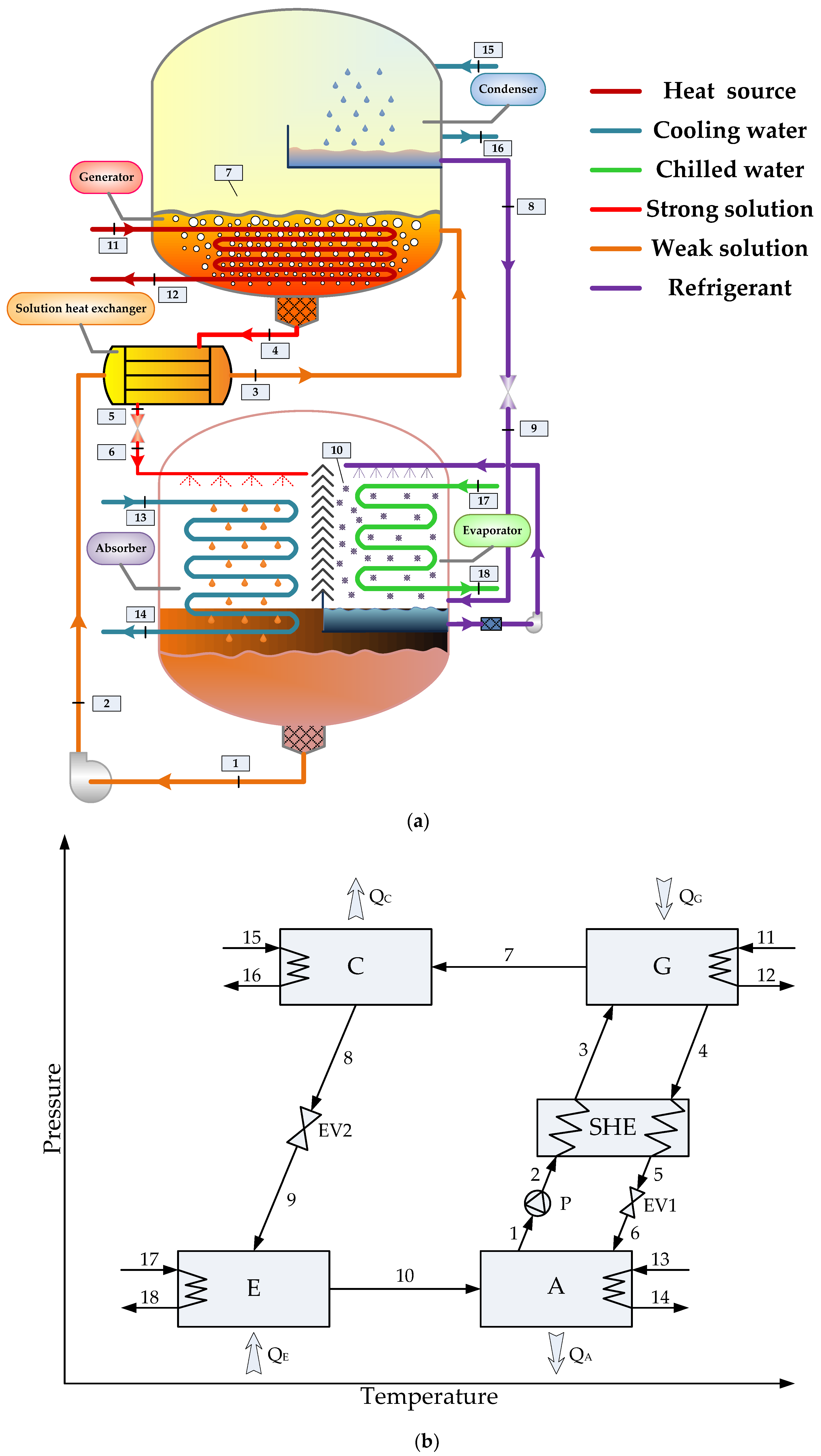
2. System Description

Figure 1a displays the schematic diagram of a single-effect ARS and the process of the cooling effect generation driven by heat sources. For mathematical modeling of the system, its main components and state points are described using the pressure–temperature coordinates in Figure 1b. It involves two pressure levels: the generator (G) and condenser (C) operate at high pressure, and the absorber (A) and evaporator (E) work at low pressure level. The high temperature heat source (stream 11–12) adds heat in the generator to separate water vapor from the weak solution (stream 3). Then, the refrigerant vapor (stream 7) from the generator is condensed by the cooling water (stream 15–16) in the condenser. Afterwards, the liquid refrigerant (stream 8) flows through an expansion valve (EV2) to the evaporator and vaporizes at the saturation temperature to absorb heat from the chilled water (stream 17–18). Subsequently, the refrigerant vapor (stream 10) is conducted to the absorber, where it is absorbed by the strong solution (stream 6) going through the solution expansion valve (EV1) and the whole process is cooled down by cooling water (stream 13–14). Finally, the low concentration solution at the outlet of the absorber (stream 1) is pumped to the generator via a solution heat exchanger (SHE). The pressurized solution (stream 2) is preheated in the SHE by the high-temperature strong solution (stream 4–5) coming from the generator.

3. Mathematical Modeling

3.1. Model Assumptions

In order to conduct the theoretical analysis of the model, some assumptions were made [12,19,22,23,24]. First, it was assumed that the entire system ran under steady state conditions and all the thermodynamic variables were homogenous within each component. Then, the solutions flowing out of the generator and absorber were considered to be saturated in equilibrium conditions at their respective temperature and pressure. Also, the refrigerant leaving the condenser and evaporator were in a saturated phase at the corresponding pressure. In addition, the pressure drop and heat loss in the components of the system were not considered, and neither was the work of the solution pump. At last, fluids passing through the expansion valves were regarded as adiabatic and isenthalpic. Additionally, the reference system was taken at 25 °C and 1 atmospheric pressure.

3.2. Thermodynamic Formulations

For the thermodynamic analysis of an ARS, the principles of mass and species conservation, as well as energy conservation including performance criteria, were applied. Each component of the chiller could be treated as a control volume with its inlet and outlet streams. The general equations of these principles must be fulfilled in all the components, where more specifics are presented as follows.

Mass balance:

$${\displaystyle \sum m_{i,in,k}}-{\displaystyle \sum m_{i,out,k}}=0$$

(1)

Species balance:

$${\displaystyle \sum m_{i,in,k}{x}_{j,i,k}}-{\displaystyle \sum m_{i,out,k}{x}_{j,i,k}}=0$$

(2)

Energy balance:

$${\displaystyle \sum H_{i,in,k}}-{\displaystyle \sum H_{i,out,k}+{\displaystyle \sum Q_{u,k}}-{\displaystyle \sum W_k}}=0$$

(3)

$${\displaystyle \sum Q_{u,k}}={\displaystyle \sum H_{u,in,k}}-{\displaystyle \sum H_{u,out,k}}$$

(4)

Equations (1) and (2) represent the mass and species balances applied to the component k (G, A, C, E, SHE) and ensure that the amounts of each substance j (LiBr, LiCl, water) entering into component k equal the total amount of j leaving k. The energy balance in Equation (3) reflects that the difference between the inlet and outlet energy flows of stream i add the heat supplied by external utility u must be equal to the work done by the component k. In these equations, m indicates the mass flow rate of stream i (kg·s⁻¹), x denotes mass fraction of substance j in stream i (kg·kg⁻¹), H is the energy flow rate (kW), Q refers to the heat transfer capacity (kW), and W represents power (kW).

According to Equations (1) and (2), the mass balance equation and species balance equation in the generator and absorber can be expressed as the following Equations (5) and (6), respectively:

$$m_{ws}=m_{ss}+m_r$$

(5)

$$m_{ws}{x}_{ws}=m_{ss}{x}_{ss}$$

(6)

The circulation ratio CR is an important parameter, which is defined as the ratio of mass flow rate of weak solution coming from the absorber to the mass flow rate of the refrigerant:

$$CR=\frac{m_{ws}}{m_r}$$

(7)

According to Equations (5) and (6), Equation (7) can be expressed as:

$$CR=\frac{x_{ss}}{x_{ss}-x_{ws}}$$

(8)

In the thermodynamic analysis of the absorption cycle, we focus on the relationship between the concentration and temperature of solution in the generator or absorber and temperature of water in the condenser or evaporator under relevant pressure. In order to simplify the calculation process, the Dühring equation is recommended for dealing with the equilibrium temperature t of a solution and the dew temperature t_s at the corresponding pressure, shown as follows:

$$t^K=a{t}_s^K+b$$

(9)

In the above equation, superscript K represents the Kelvin temperature scale, and a and b are the functions of solution composition. For LiBr-H₂O and LiCl-H₂O, a and b can be approximately expressed by a linear function of solution concentration in a moderately narrow concentration range. Then, Equation (9) can be rewritten as:

$$t^K=\left(a_{0}x+a_1\right)t_s^K+\left(b_{0}x+b_1\right)$$

(10)

where a₀, a₁, b₀, and b₁ are constants in the concentration range. The constants above are 0.538, 0.845, 48.3, and −35.6 in sequence for a LiBr-H₂O equilibrium solution according to Kim and Infante Ferreira’s study [15]; likewise, 0.304, 0.988, 59.3, and −27.9 are used for LiCl-H₂O equilibrium solution based on Conde’s study [14]. The absolute error is less than 1 K for LiBr-H₂O and 1.8 K for LiCl-H₂O within the operating range. Actually, the concentration of the solution varies in the range of ≈0.5–0.65 for LiBr-H₂O and ≈0.4–0.5 for LiCl-H₂O in the whole research process. Thus, the Dühring equation completely meets the requirement of computational accuracy.

In this paper, Kim and Infante Ferreira’s method [32] is referred to when calculating the heat flows of components so as to facilitate the following iterative computations. This method is derived from Haltenberger’s formula where the solution enthalpy at one concentration can be calculated from that of another concentration in the same solution temperature. Meanwhile, the partial specific enthalpy of the refrigerant takes an approximate value under a low-pressure condition. Finally, the heat load of each component can be expressed using the following formulas:

Generator:

$$Q_G=m_{ws}{c}_{p,ws}(t_4-t_3)+m_r\left[{\overline{\chi }}_G{h}_{co}+c_{p,r}^v\left(t_7-t_4\right)\right]$$

(11)

where ${\overline{\chi }}_G$ is defined using:

$${\overline{\chi }}_G={\left(\frac{t_{3\mathrm{a}}+t_4}{2t_8}\right)}^2\frac{1}{a_0\left(x_{ws}+x_{ss}\right)/2+a_1}$$

(12)

Absorber:

$$Q_A=m_{ws}{c}_{p,ws}(t_5-t_1)+m_r\left[{\overline{\chi }}_A{h}_{ev}+c_{p,r}^v\left(t_{10}-t_1\right)-c_{p,ss}\left(t_5-t_{6\mathrm{a}}\right)\right]$$

(13)

where ${\overline{\chi }}_A$ is defined using:

$${\overline{\chi }}_A={\left(\frac{t_{6\mathrm{a}}+t_1}{2t_{10}}\right)}^2\frac{1}{a_0\left(x_{ws}+x_{ss}\right)/2+a_1}$$

(14)

Condenser:

$$Q_C=m_r\left[h_{co}+c_{p,r}^v\left(t_7-t_8\right)\right]$$

(15)

Evaporator:

$$Q_E=m_r\left[h_{ev}-c_{p,r}^l\left(t_8-t_{10}\right)\right]$$

(16)

Solution heat exchanger:

$$Q_{SHE}=\left(m_{ws}-m_r\right)c_{p,ss}(t_4-t_5)=m_{ws}{c}_{p,ws}\left(t_3-t_2\right)$$

(17)

In order to make it more precise for application, some empirical formulations used to describe the thermodynamic properties of working pairs are adopted by this model instead of constant values. The latent heat of evaporation and condensation in different temperatures are calculated from Wagner et al. [33]. The specific heat of LiBr-H₂O and LiCl-H₂O solutions are computed using the correlations of Patek and Klomfar [17,18].

The system energetic performance is represented in terms of COP. It is defined as the ratio of cooling capacity to the heat input and is presented in Equation (18) [19,21]:

$$COP=\frac{Q_E}{Q_G}$$

(18)

The Carnot coefficient of performance (COP_c) represents the maximum possible coefficient of the ARS, as shown in Equation (19) [34]:

$$CO{P}_c=\left(\frac{t_4^K-t_1^K}{t_4^K}\right)\left(\frac{t_{10}^K}{t_8^K-t_{10}^K}\right)$$

(19)

By comparing the COP with COP_c, the efficiency ratio is given as:

$${\eta }_{eff}=\frac{COP}{CO{P}_c}$$

(20)

The exergetic efficiency of the chiller is the ratio of the exergy produced in the evaporator to the exergy supplied to the generator. It can be written as [21]:

$${\eta }_{ex}=\frac{Q_E\left|\left(1-\frac{t_0^K}{t_E^K}\right)\right|}{Q_G\left(1-\frac{t_0^K}{t_G^K}\right)}$$

(21)

3.3. Standard Design of Absorption Chiller with LiBr-H₂O/LiCl-H₂O Working Pair

This section intends to design the single effect absorption chiller using LiBr-H₂O and LiCl-H₂O. The main components of the absorption chiller (generator, absorber, condenser, evaporator, and solution heat exchanger) are virtually five heat exchangers. The objective of the design is to determine the heat transfer characteristics of each component and mass flow rate of each state point under the condition that the cooling capacity and design parameters in both chillers are the same.

The heat transfer model of the heat exchanger in each component (k) can be described by the overall heat transfer coefficient-area product (UA) and the logarithmic mean temperature difference (Δt^lm), shown as follows:

$$Q_k={(UA)}_k\Delta t_k^{lm}$$

(22)

In the above formula, the logarithmic mean temperature difference can be calculated conveniently with high-precision by employing Chen’s approximation [35,36], which is described as a function of temperature differences between the hot and cold end, as shown in the following equation:

$$\Delta t_k^{lm}\cong {\left[\Delta t_k^h\Delta t_k^c\frac{\Delta t_k^h+\Delta t_k^c}{2}\right]}^{\raisebox{1ex}{$1$}\!\left/ \!\raisebox{-1ex}{$3$}\right.}$$

(23)

According to the energy balance equations shown in Equations (3) and (4), heat transfer rates of the main components can be expressed in terms of energy flow rates of external utilities, as in the following Equations (24)–(27):

$$Q_G=m_{11}{c}_{p,w}\left(t_{11}-t_{12}\right)$$

(24)

$$Q_A=m_{13}{c}_{p,w}\left(t_{14}-t_{13}\right)$$

(25)

$$Q_C=m_{15}{c}_{p,w}\left(t_{16}-t_{15}\right)$$

(26)

$$Q_E=m_{17}{c}_{p,w}\left(t_{17}-t_{18}\right)$$

(27)

In this study, the rated cooling load of the absorption chiller was 50 kW. The effectiveness of heat exchanger was set at 0.7. To carry out the design of the absorption chiller, the temperature of each state point in the operating conditions should be determined at first. An absorption chiller contains three external circuit flows: hot water, cooling water, and chiller water. The states of these fluids are closely related to the actual environment, especially inlet temperatures. Once the inlet temperatures of external fluids are selected, temperatures of the other points can be typically determined by some increments or decrements. In accordance with References [22,23,34], the design specifications applied in this paper for both systems are shown in

Table 1. Design temperatures of state points in the components.

Component	State Point	Symbol	Value
Generator	Inlet temperature of hot water (°C)	t11	90
	Outlet temperature of hot water (°C)	t12 = t11 − 7	83
	Outlet solution temperature from generator (°C)	t4 = t12 − 3	80
Absorber	Inlet temperature of cooling water (°C)	t13	30
	Outlet temperature of cooling water (°C)	t14 = t13 + 5	35
	Outlet solution temperature from absorber (°C)	t1 = t14 + 3	38
Condenser	Inlet temperature of cooling water (°C)	t15	30
	Outlet temperature of cooling water (°C)	t16 = t15 + 5	35
	Condensation temperature (°C)	t8 = t16 + 3	38
Evaporator	Inlet temperature of chilled water (°C)	t17	13
	Outlet temperature of chilled water (°C)	t18 = t17 − 5	8
	Evaporation temperature (°C)	t10 = t17 − 7	6

:

After setting up these temperatures, the mass flow rate of each point, as well as the heat transfer characteristics and heat load of each component, could be determined from the above equations. In most studies, temperature differences between the fluids in Table 1 are treated as constant to research the operation performance of an absorption chiller, which is in fact at variance with the actual situation. In the next section, a new effective method has been developed to overcome this problem.

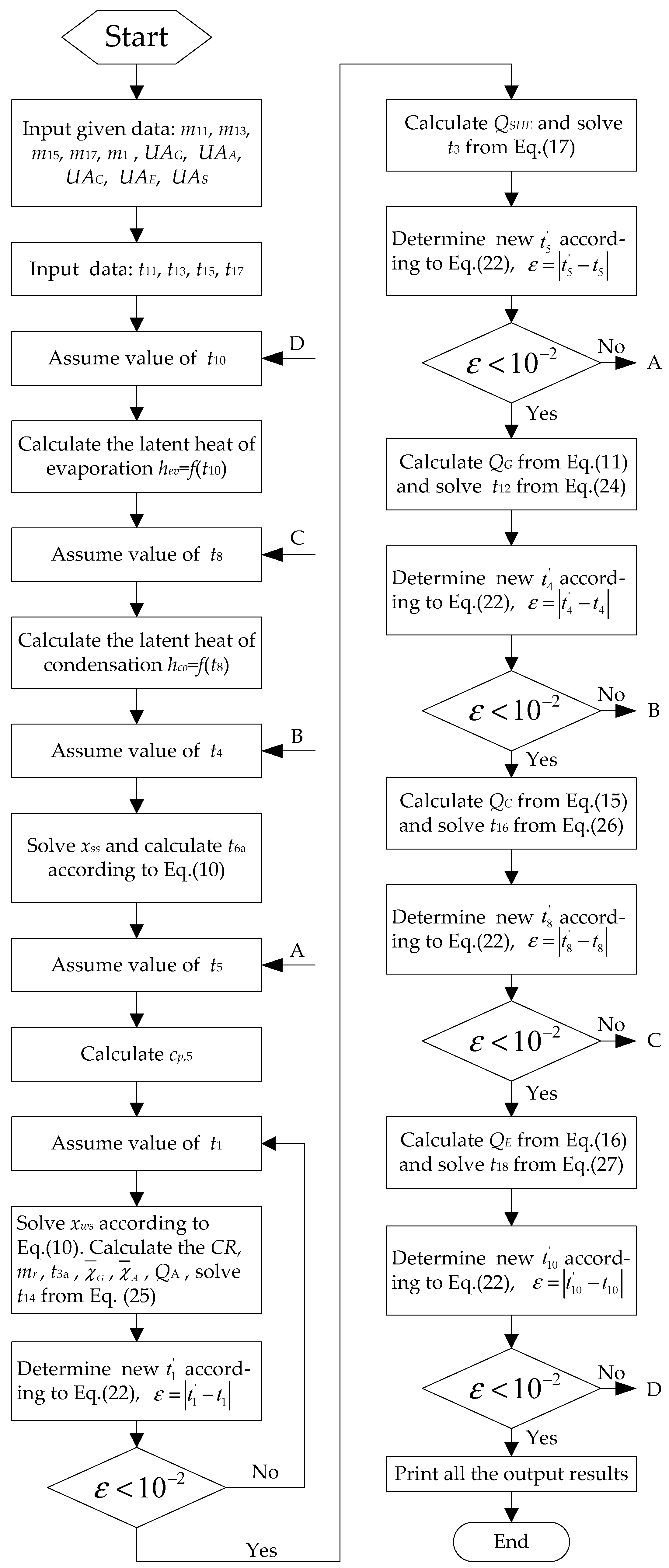
3.4. Calculation Procedure of Absorption Chiller under Design Features

In the control volume of the absorption chiller, heat transfers of components take place between the external circuit flows (hot, cold, and chilled water) and its internal circuit flows (the refrigerant and the LiBr-H₂O/LiCl-H₂O solution). It is more practical to evaluate the influences of external fluids on the absorption chiller. In order to build a model that could be commonly used, the heat transfer characteristics (UA) of all the components are assumed to be invariable within the entire operating range, just as in References [12,37,38,39]. According to the research, selecting the design parameters is adequate to simulate the real situation with a good approximation because the overall heat transfer coefficients vary within a narrow range most of the time [12]. In particular for this study, the mass flow rates of the solution pump and external circuit flows are kept constant in an attempt to minimize its effects on the overall heat transfer coefficients, so it allows for comparison of the results obtained from the LiBr-H₂O and LiCl-H₂O absorption chillers. A computer program in Matlab language (Matlab R2014a, The MathWorks Inc., Natick, MA, America) has been made to carry out the simulation. Figure 2 shows a flow chart of the computer program (see in Supplementary Materials).

As shown in the simulation procedure, it contains a five-step iteration of different temperatures corresponding to the main components of the chiller. In this way, it is effective to describe the operation of chiller and evaluate the influences of external circuits on its overall performance. According to the studies on thermodynamic properties of the working pairs, the vapor pressure of solution (P) is calculated using an empirical formulation, which is described as the function of solution temperature (t) and mass fraction (x), i.e., P = f(t, x). In the mathematical modeling of the system, the vapor pressure of the solution equals to the saturation pressure of water in the condenser or evaporator, P = f(t_s). As a result, in the most cases, the temperature and pressure of solution are acquired to solve its mass fraction, x = f(P, t). The complex multivariable nonlinear equations hinder the iterative computation of the solution parameter immensely.

The method in this study using Dühring equation shown as Equation (10) completely avoids the problem and makes it much easier to deal with the relation between the solution temperature and mass fraction. Besides, in the heat transfer model, the logarithmic mean temperature difference is calculated using Equation (23) with a high accuracy. In this process, the logarithmic equation is converted into an algebraic equation, which provides a simple way to solve for the fluid temperature. Consequently, the developed method in this study will reduce the amount of computation compared with the conventional enthalpy-based calculation. In conclusion, the established model is efficient and convenient to predict the performance of an absorption chiller, especially for alternative working pairs without specific information.

4. Results and Discussion

4.1. Validation of the Model

In order to validate the developed model, the simulation results are compared with related research reported by Anand and Kumar [40] and Kaushik and Arora [41] for a LiBr-H₂O system, and Patel and Pandya [20] for a LiCl-H₂O system. In the comparison, the values of input parameters (mainly the temperatures of the components and mass flow rate of the refrigerant) in the examined cases were identical. According to the references, for LiBr-H₂O system, the input values were set as: t_G = 87.8 °C, t_A = t_C = 37.8 °C, t_E = 7.2 °C, ε = 0.7, m_r = 1 kg·s⁻¹. In the LiCl-H₂O system, the parameters were as follows: t_G = 78 °C, t_A = 40 °C, t_C = 36 °C, t_E = 10 °C, ε = 0.7, m_r = 0.00148 kg·s⁻¹.

It was observed that the simulation results of the present work agreed well with the references’ data and the differences between them were within ±1% for a LiBr-H₂O system and ±3% for a LiCl-H₂O system. In the two systems, the maximum difference percentage of heat capacity all occurred in the absorber (0.8% and 2.6% respectively), which produces no effect on COP. The details are presented in

Table 2. Comparisons of energy analysis of present work with references’ data.

		LiBr-H2O					LiCl-H2O
Name	Symbol	Anand [40]	Kaushik [41]	Present Work	Difference Percentage (%) with Anand	Difference Percentage (%) with Kaushik	Patel [20]	Present Work	Difference Percentage (%) with Patel
Heat capacity of generator (kW)	QG	3073.11	3095.70	3074.45	0.04	−0.69	4.465	4.519	1.21
Heat capacity of absorber (kW)	QA	2922.39	2945.27	2945.90	0.80	0.02	4.268	4.379	2.6
Heat capacity of condenser (kW)	QC	2507.89	2505.91	2504.22	−0.15	−0.07	3.705	3.691	−0.38
Heat capacity of evaporator (kW)	QE	2357.17	2355.45	2355.93	−0.05	0.02	3.517	3.505	−0.34
Coefficient of performance	COP	0.7670	0.7609	0.7663	−0.09	0.71	0.7877	0.7758	−1.51

. It proves that the calculation model is valid and reliable.

4.2. Sensitivity Analysis of the Design Parameters

From the results and mathematical models in previous studies, it indicates that the performance of a single effect absorption system mainly depends on the selection of main design parameters such as absorber temperature t₁, generator temperature t₄, condenser temperature t₈, evaporator temperature t₁₀, and heat exchanger effectiveness [34].

In this section, the sensitivity analysis of these parameters is conducted to examine the effect on LiBr-H₂O and LiCl-H₂O ARS performances. The method of control variables was employed for the sensitivity analysis, where one of the system parameters is varied while the other parameters were kept constant. The purpose of this simulation was to predict the most efficient pair and determine the operating temperature range. The results are shown in the following (see in Supplementary Materials).

4.2.1. Effect of Generator Temperature on System

Figure 3 and Figure 4 present the variations of the coefficient of performance (COP) and efficiency ratio (η_eff) with generator temperature (t₄) in LiBr-H₂O and LiCl-H₂O systems. The system performance was analyzed under three different condenser and absorber temperature levels (32 °C, 36 °C, and 40 °C) in order to cover a greater range of operating conditions. In this process, the absorption temperature was set equal to condensation temperature (t₁ = t₈).

As shown in Figure 3 and Figure 4, it is obvious that the LiCl-H₂O working pair displayed better performances than LiBr-H₂O in the operating range of examined cases. It can be observed that both the COP and efficiency ratio value increased sharply with generator temperature initially, but COP tended to level off and even drops somewhat rather than show an apparent decline in the efficiency ratio curves with a further increase in generator temperature. Moreover, a lower condensation and absorption temperature led to a greater COP in the same generator temperature and the maximum value approximated to 0.8 for both working pairs. These curves reflect that there existed a minimum generator temperature in every case that brought about an adequate COP in the application of absorption system. Furthermore, it can be inferred that this minimum generator temperature was closely related to the maximum efficiency ratio of system, as the calculated results show.

In Figure 4, each curve of the efficiency ratio in the two systems had almost the same tendency, no matter the limitations, just like the curves moving in the direction of generator temperature increasing, and there existed almost the same maximum values with 0.68 for LiBr-H₂O and 0.7 for LiCl-H₂O for an intermediate generator temperature for each curve. The reason for this maximum efficiency ratio is the system COP_c increased with the generator temperature, but the COP curve almost flattened.

It is also useful to state that higher generator temperatures must match higher condensation and absorption temperatures because of the solubility limitation of the two working pairs. Although it has a greater performance than the LiBr-H₂O system, the LiCl-H₂O system is only allowed to operate in a much smaller range of working conditions, which primarily limits its application.

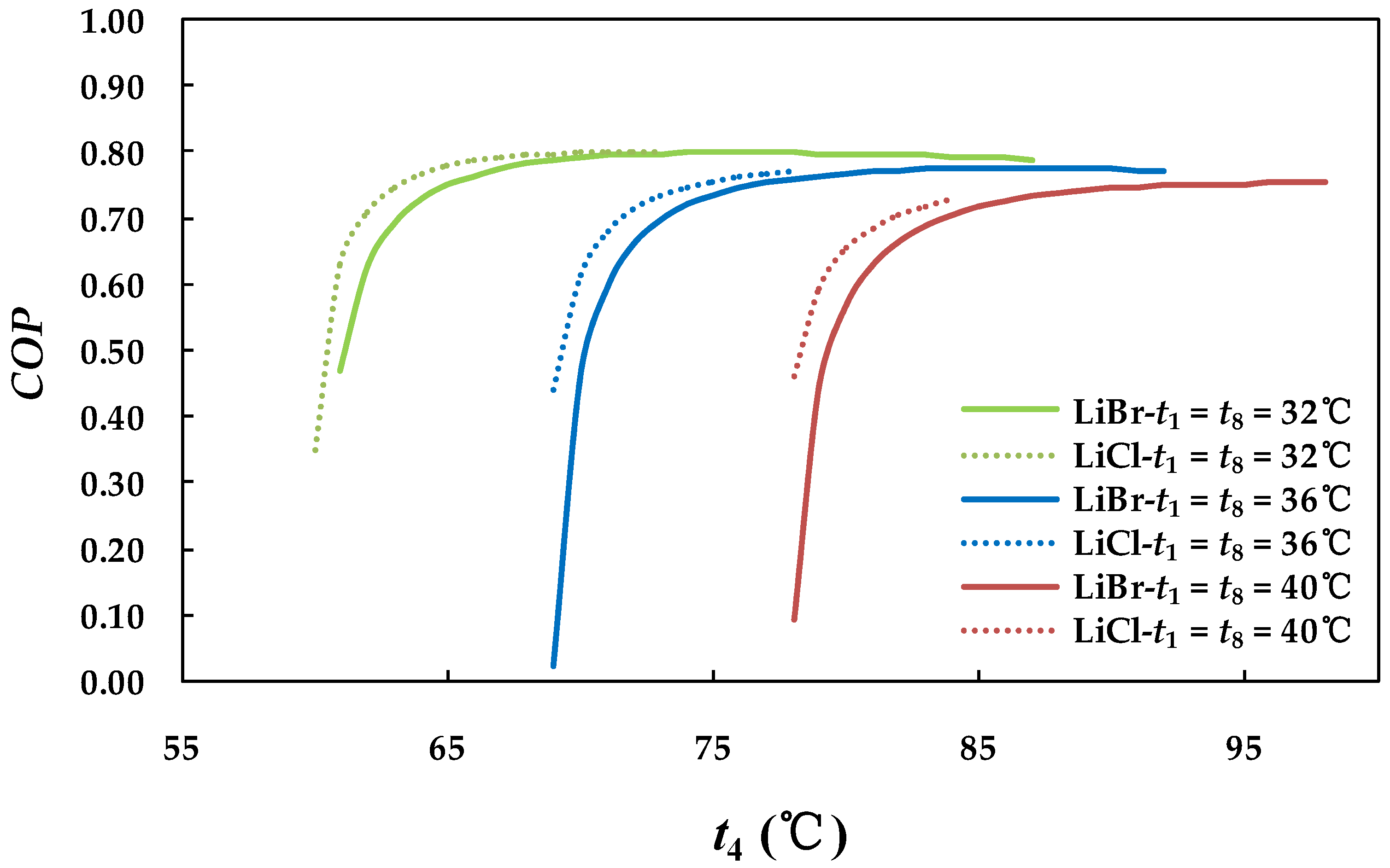
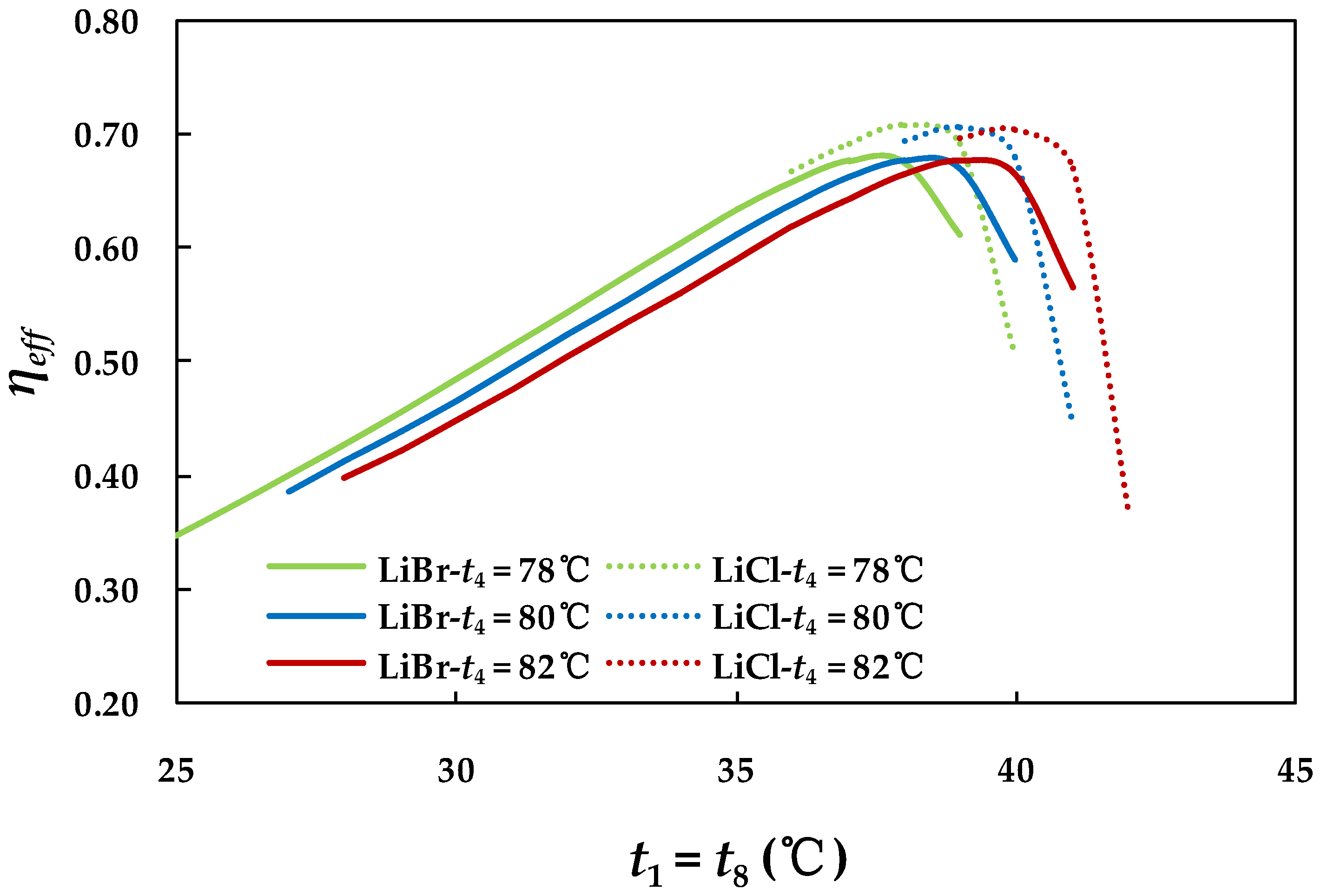
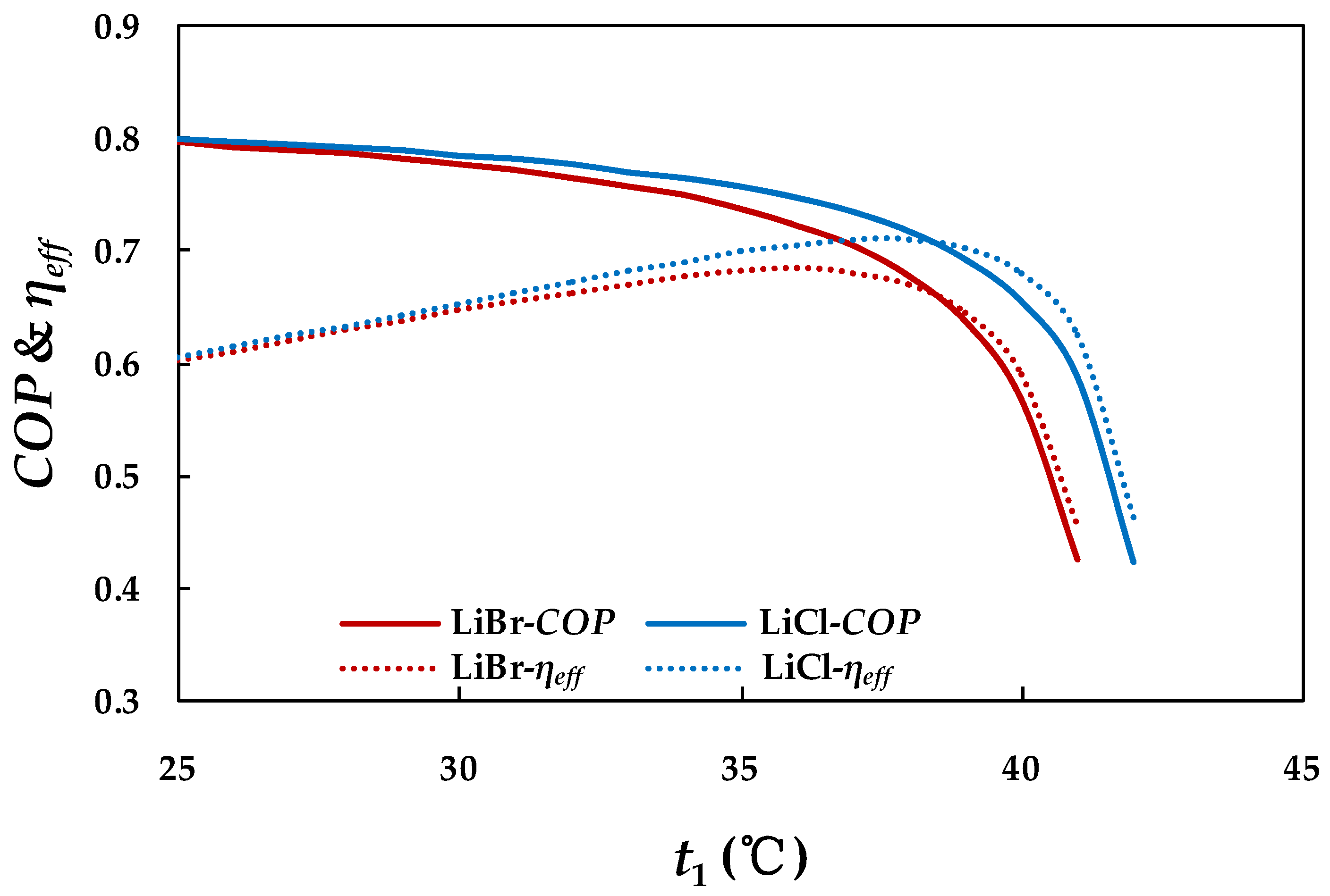
4.2.2. Effect of Absorber and Condenser Temperatures on System

The effects of the variation in the absorber and condenser temperatures on the system COP and efficiency ratio are illustrated in Figure 5 and Figure 6. It can be observed that LiCl-H₂O was the working pair with the higher performance but had an extreme operating range that was suitable only for higher condensation and absorption temperatures, and the performance declined significantly with the temperature increasing. Conversely, LiBr-H₂O system was more adaptable for working conditions varying in a large range. When the generator temperature was kept at 80 °C, the LiCl-H₂O absorption cycle could only run in the condenser and absorber temperatures range of 38–41 °C, compared with 27–40 °C in the LiBr-H₂O absorption cycle. Especially, the COP of the LiBr-H₂O system kept basically in line at a high level close to 0.8 for all cases under a lower condensation and absorption temperature no matter the generator temperature changes. However, the curves of the efficiency ratio were clearly different, as shown in Figure 6, because they were maximized for a specific generator temperature in every case. In the examined cases, the maximum values of the efficiency ratio were nearly the same, which was about 0.67 for the LiBr-H₂O system and 0.70 for the LiCl-H₂O system.

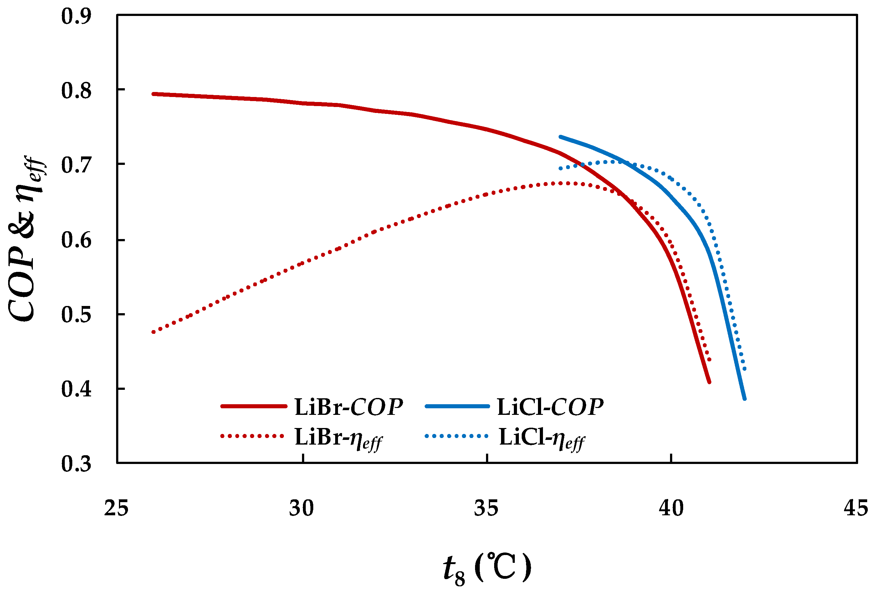
4.2.3. Effect of Absorber and Condenser Temperatures on System

Figure 7 and Figure 8 depict the effect of the condenser or absorber temperature on COP and the efficiency ratio in both systems. It can be seen that a decrease in COP and the efficiency ratio occurred when increasing either of the temperatures. Moreover, the performances of both systems degraded more excessively in the high temperature zone.

Comparing the results of two working pairs from Figure 7 and Figure 8, it is shown that, for the LiCl-H₂O pair, the absorber temperature was allowed a wide range when condenser temperature was set at 40 °C, which was not true for the absorber temperature. Therefore, a conclusion can be reached that the condenser temperature had the greater impact on the LiCl-H₂O system. If the condenser temperature was too small, the system had operating trouble because the concentration of strong solution got larger, which led to solution crystallization. On the other hand, the concentration of strong solution became lower with the condenser temperature increasing, which brought about the solution cycle ratio increase at a constant cooling capacity, and eventually resulted in the degradation of system performance for the heat load of a generator rising rapidly. There also existed a maximum value in each of the efficiency ratio curves and the corresponding temperatures in LiCl-H₂O system were higher. This suggests that the LiCl-H₂O working pair was superior to LiBr-H₂O under the condition with a relatively higher condenser or absorber temperature. However, both of the systems were sensitive to overly high temperatures in the condenser or absorber, and the performance declined sharply. As such, the cooling water temperature should be strictly controlled to maintain a proper condenser and absorber temperature.

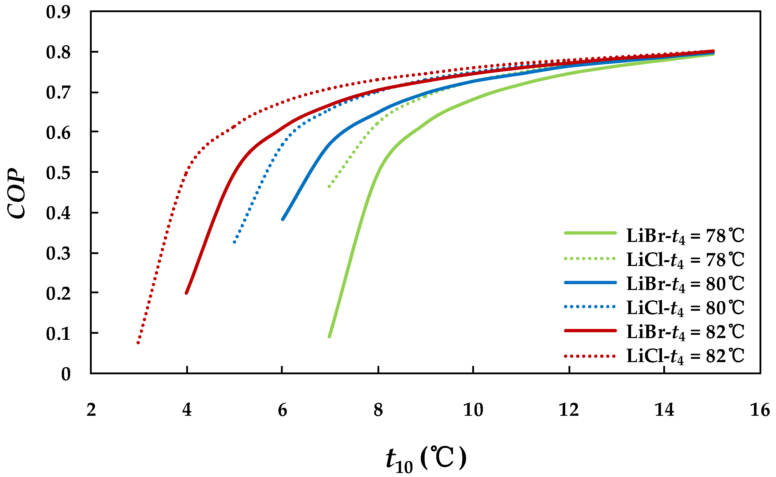
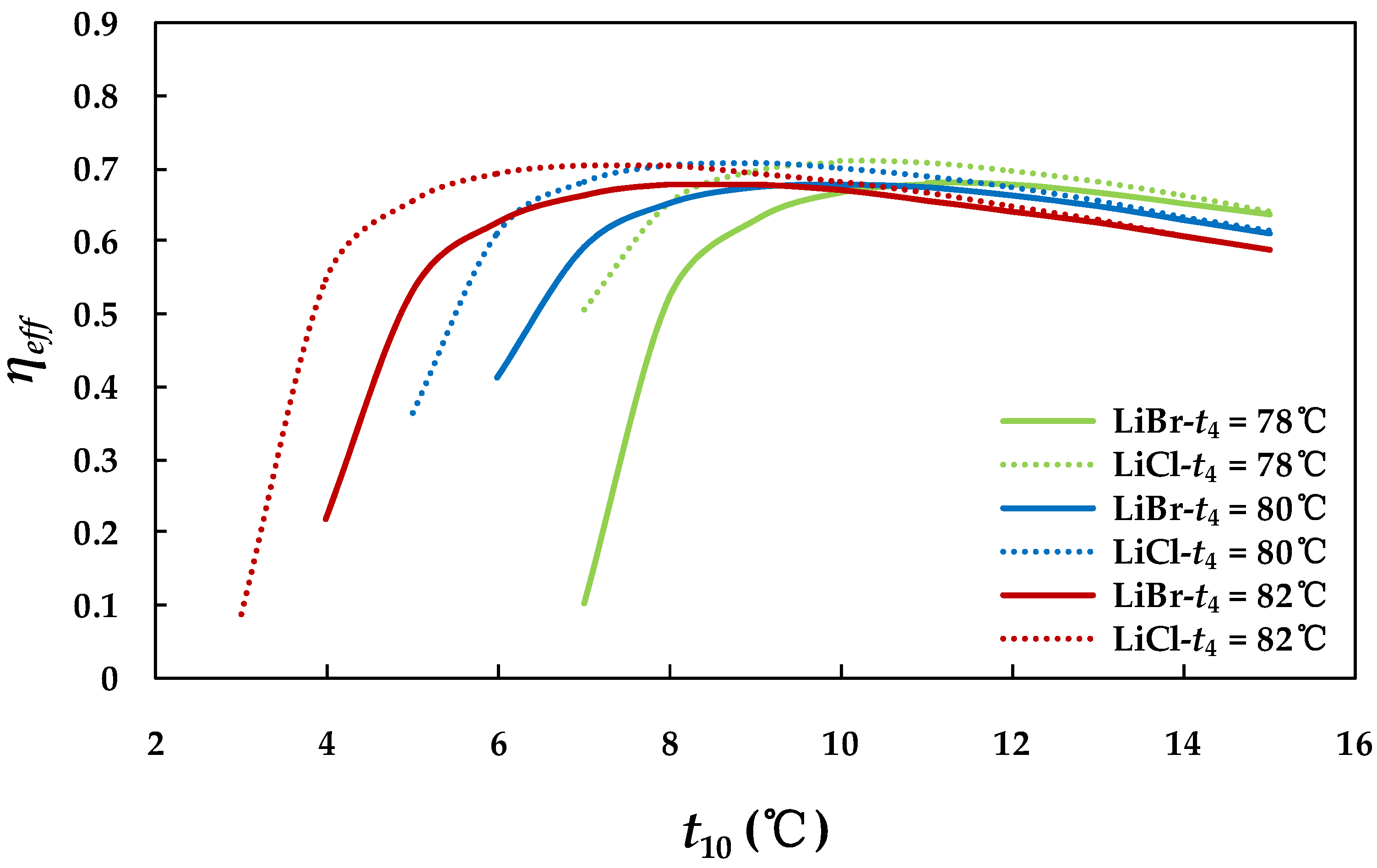
4.2.4. Effect of Evaporator Temperature on System

The variations of COP with evaporator temperature in the two systems are shown in Figure 9. It can be seen that the COP of both systems increased with evaporator temperature, but the growth rate was weakened and all the values approached 0.8 eventually. At this point, it is also important to state that a higher generator temperature was demanded to generate a lower evaporator temperature effect because the cooling production was harder to be achieved with low grade energy. Moreover, the COP was greater in the higher generator temperature at the same evaporator temperature level.

In Figure 10, it can be seen that each curve of the efficiency ratio had a maximum value according to the generator temperature level. To explain the maximum points of the efficiency ratio curves, a higher evaporating temperature or generator temperature level led to a higher COP_c according to Equation (19) and the growth rate of COP_c was greater than COP with the evaporating temperature increasing for each curve. At the higher evaporator temperature condition, the COP_c played the dominant role in the efficiency ratio because the COP values were almost the same in these cases.

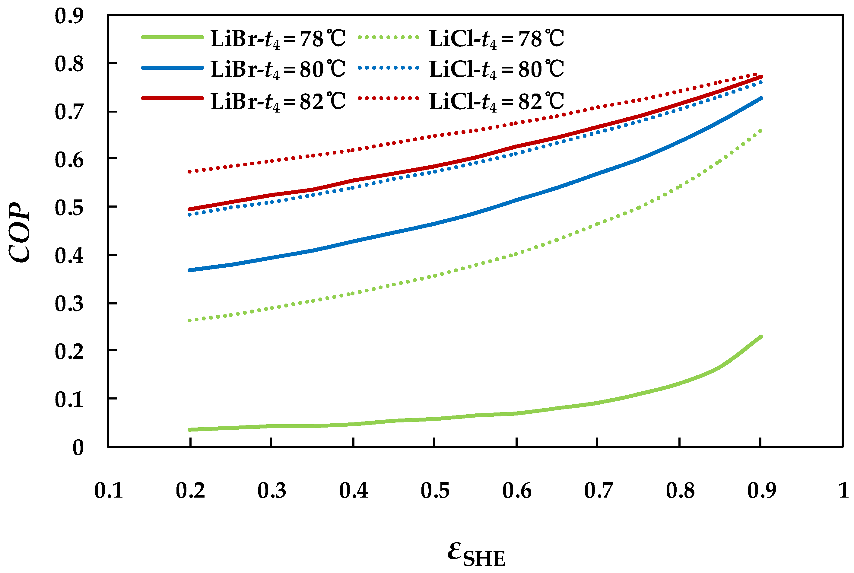
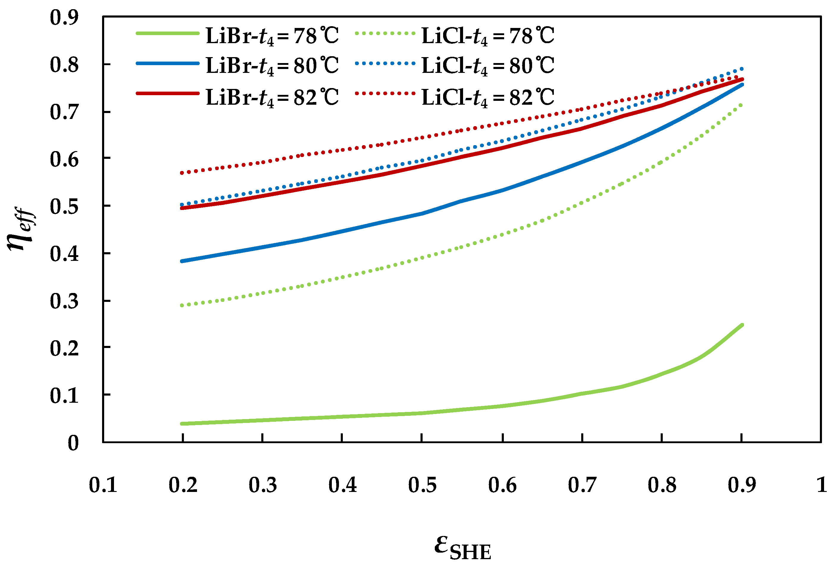
4.2.5. Effect of Effectiveness of Solution Heat Exchanger on System

Figure 11 and Figure 12 present the system performance in terms of COP and efficiency ratio varying with the solution heat exchanger effectiveness in the two systems. It can be seen that the effectiveness of the solution heat exchanger had a great impact on the system performance, especially at the lower generator temperature. This makes sense because the higher solution heat exchanger effectiveness improved the heat transfer between the generator and absorber and decreased the outside heat input and dissipation. Besides, LiCl-H₂O system had a great advantage over LiBr-H₂O at a lower generator temperature level, and the results agree with previous conclusions.

The performances of the two absorption cycles go up steadily with the heat exchanger effectiveness increasing, but to a markedly larger extent in the higher section. The tendency of the efficiency ratio is similar to the COP curve because the COP_c value was nearly at 1 in all examined cases. With the increase of the generator temperature, the gap between the two systems diminished. It is also obvious that the temperature of the weak solution leaving the solution heat exchanger decreased as the effectiveness rose, which indicates that the chances of solution crystallization increased.

4.3. Analysis of the Two Absorption Chillers at Off-design Conditions

In the actual operation of a designed absorption chiller, the working conditions of the external circuit flows varies with the ambient conditions and the performance and each state point parameter of the chiller will change. Thus, it is necessary to examine the influence of the external circuit flows on the chiller and observe its regularity for practical application. In this work, the approach for the cycle simulation was carried out to establish a set of state points of the system and change the relevant parameters of external circuit fluids around it. Furthermore, the design features, particularly the heat transfer characteristics of the heat exchangers, had a decisive effect on the absorption chiller performance. The operating parameters of all the state points used for the initial values of simulation are listed in

Table 3. Single effect absorption chiller operating parameters.

Point	LiBr-H2O			LiCl-H2O
	t (°C)	m (kg·s−1)	x (%)	t (°C)	m (kg·s−1)	x (%)
1	38.0	0.50039	55.858	38.0	0.25584	43.874
2	38.0	0.50039	55.858	38.0	0.25584	43.874
3	65.4	0.50039	55.858	64.6	0.25584	43.874
4	80.0	0.47914	58.335	80.0	0.23459	47.849
5	50.6	0.47914	58.335	50.6	0.23459	47.849
6	50.6	0.47914	58.335	50.6	0.23459	47.849
7	80.0	0.02125	0	80.0	0.02125	0
8	38.0	0.02125	0	38.0	0.02125	0
9	6.0	0.02125	0	6.0	0.02125	0
10	6.0	0.02125	0	6.0	0.02125	0
11	90.0	2.43054	0	90.0	2.34078	0
12	83.0	2.43054	0	83.0	2.34078	0
13	30.0	3.29257	0	30.0	3.17298	0
14	35.0	3.29257	0	35.0	3.17298	0
15	30.0	2.53054	0	30.0	2.53054	0
16	35.0	2.53054	0	35.0	2.53054	0
17	13.0	2.39232	0	13.0	2.39232	0
18	8.0	2.39232	0	8.0	2.39232	0

.

From the above operating parameters of each state point, standard working conditions of the two absorption chillers can be obtained from thermodynamic analysis, such as heat capacity (Q) and heat transfer characteristics (UA) of each component, as presented in

Table 4. Single effect absorption chiller performance parameters and design data.

Items	LiBr-H2O	LiCl-H2O
Heat transfer rate of component (kW)
Generator (QG)	71.12	68.49
Absorber (QA)	68.81	66.32
Condenser (QC)	52.89	52.89
Evaporator (QE)	50	50
Solution heat exchanger (QSHE)	27.29	18.45
COP	0.703	0.730
Heat transfer characteristics (kW·°C−1)
Generator (UAG)	5.287	4.973
Absorber (UAA)	6.049	5.829
Condenser (UAC)	10.387	10.387
Evaporator (UAE)	12.566	12.566
Solution heat exchanger (UAS)	2.009	1.323

. It can be seen that the heat load in the condenser was slightly higher than that in the evaporator and that was also higher for the generator and absorber. This was primarily due to the superheating vapor in the generator and condenser compared with the saturated vapor in the absorber and evaporator. The highest heat transfer rate occurred in the generator that was approximately 71.12 kW for LiBr-H₂O and 68.49 kW for LiCl-H₂O. As a result, the LiCl-H₂O system had a higher COP than the LiBr-H₂O system for the same design parameters.

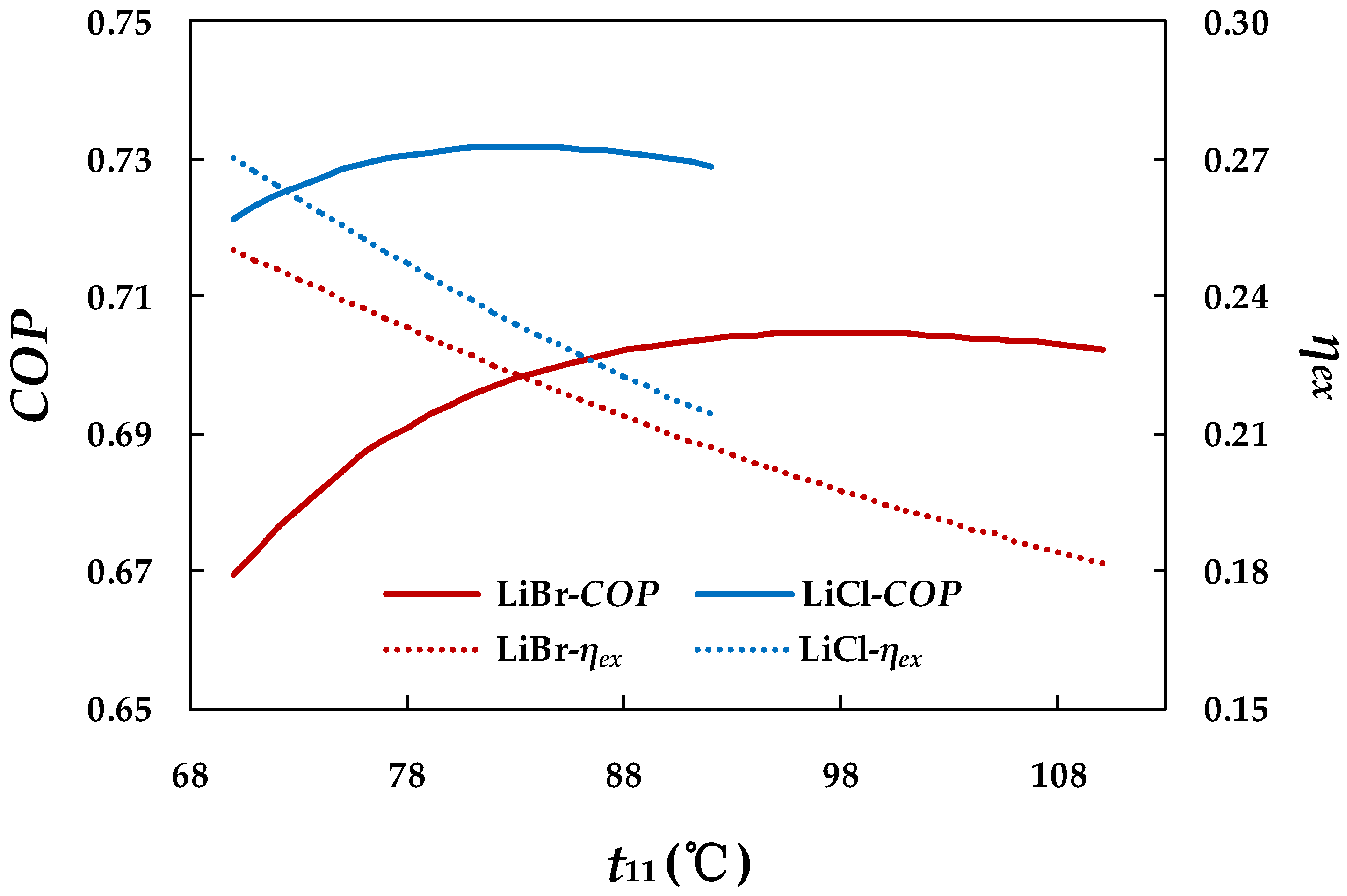
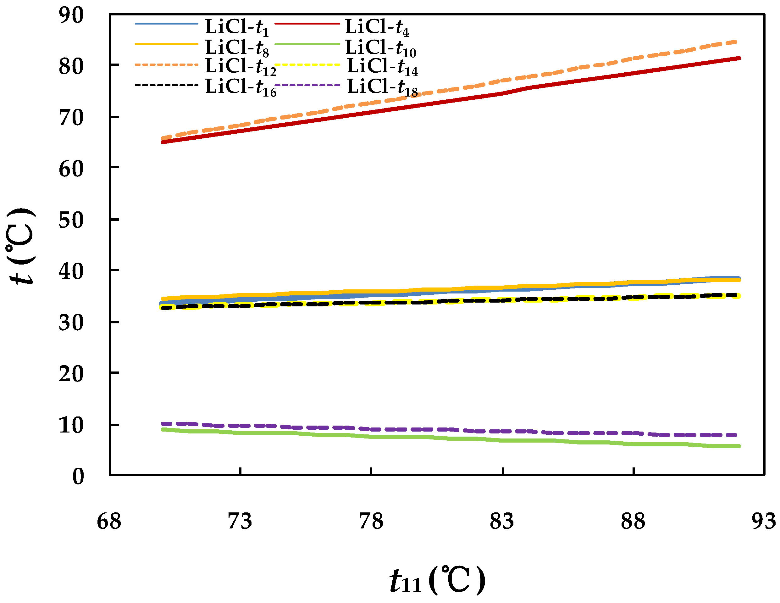
4.3.1. Effect of Hot Water Inlet Temperature in Generator

Figure 13 shows the variation of COP and exergetic efficiency with hot water inlet temperature. The COP curves of both chillers increased in the first stage but degraded a little after an intermediate temperature of about 98 °C for the LiBr-H₂O system and 83 °C for the LiCl-H₂O system, which were also the maximum values. However, the exergetic efficiency of the chiller was negatively affected by the increase of the heat source inlet temperature, dropping from about 0.25 to 0.18 for the LiBr-H₂O system and 0.27 to 0.21 for the LiCl-H₂O system in their own operating ranges.

According to Figure 14 and Figure 15, the inlet temperature of the heat source started from 70 °C and rose to 110 °C, but LiCl-H₂O system ends up at 92 °C due to a crystallization problem. With the increase in inlet temperature of the heat source water, the exit temperatures of the internal and external fluids in the main components showed close to linear growth except in the evaporator for both chillers. This was because temperatures of the refrigerant and the strong solution at the outlet of the generator increased as the heat source temperature went up, which led to the average temperatures of both condenser and the absorber increasing. Thus, for the two components, the temperature differences of heat transfer between the solution and water increased under the inlet cooling water being constant, which resulted in heat transfer rates of these components improving. As a consequence, the exit temperatures of the cooling water in the condenser and the absorber increased with constant mass flow rates and inlet temperatures. Besides, the increase of the refrigerant quantity augmented the cooling capacity in the evaporator, which accounted for the temperature of the outlet chilled water decrease because the mass flow rate and inlet temperature of chilled water were invariable. According to Equation (22), the evaporating temperature decreased eventually and also caused the corresponding low pressure level.

When the inlet temperature of the heat source water increased by 1 °C, the cooling capacity of the chiller increased by ≈1.2%–4.1% for the LiBr-H₂O system and ≈1.9%–3.9% for the LiCl-H₂O system, and the higher the temperature of the heat source, the slower the growth rate of the cooling capacity.

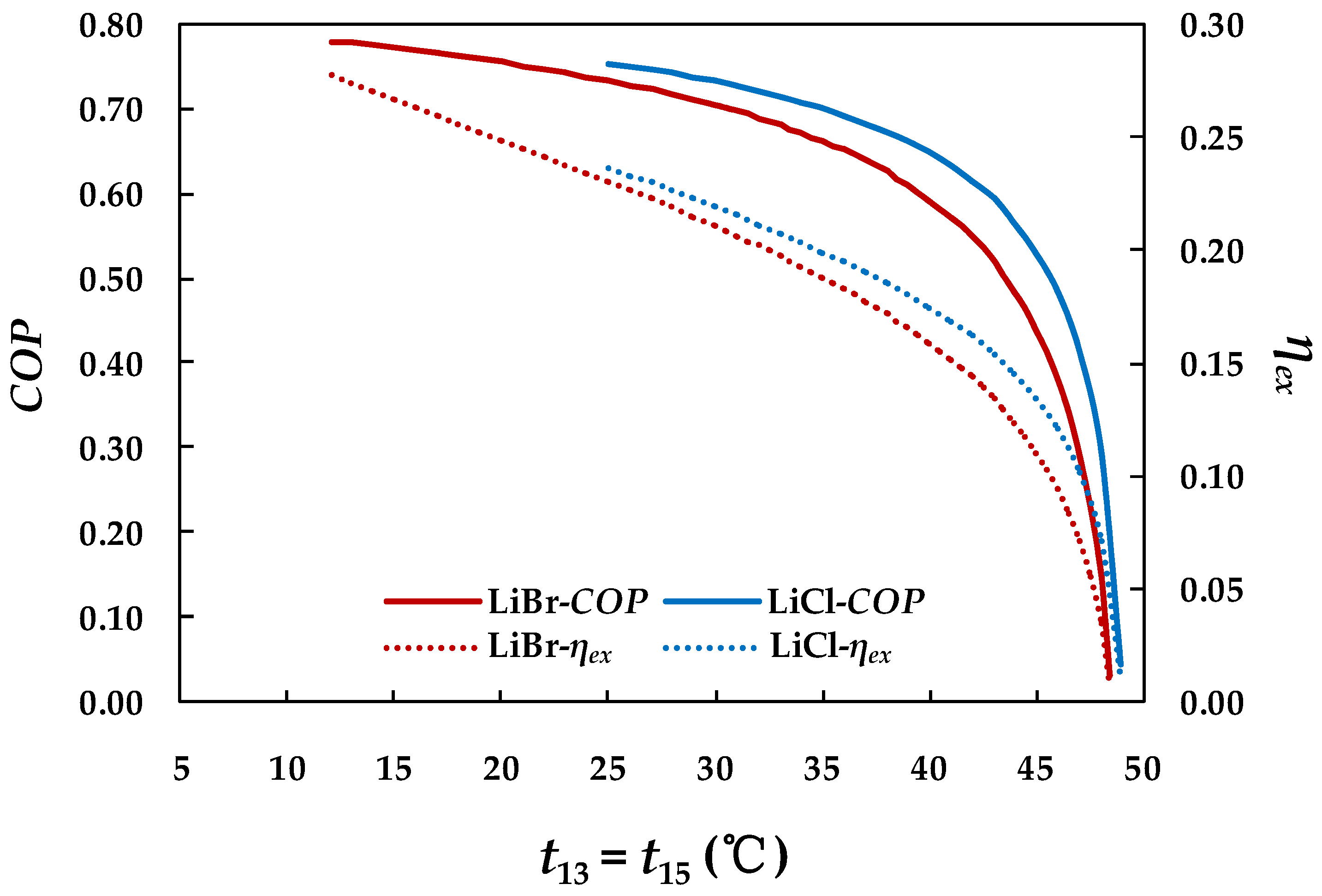
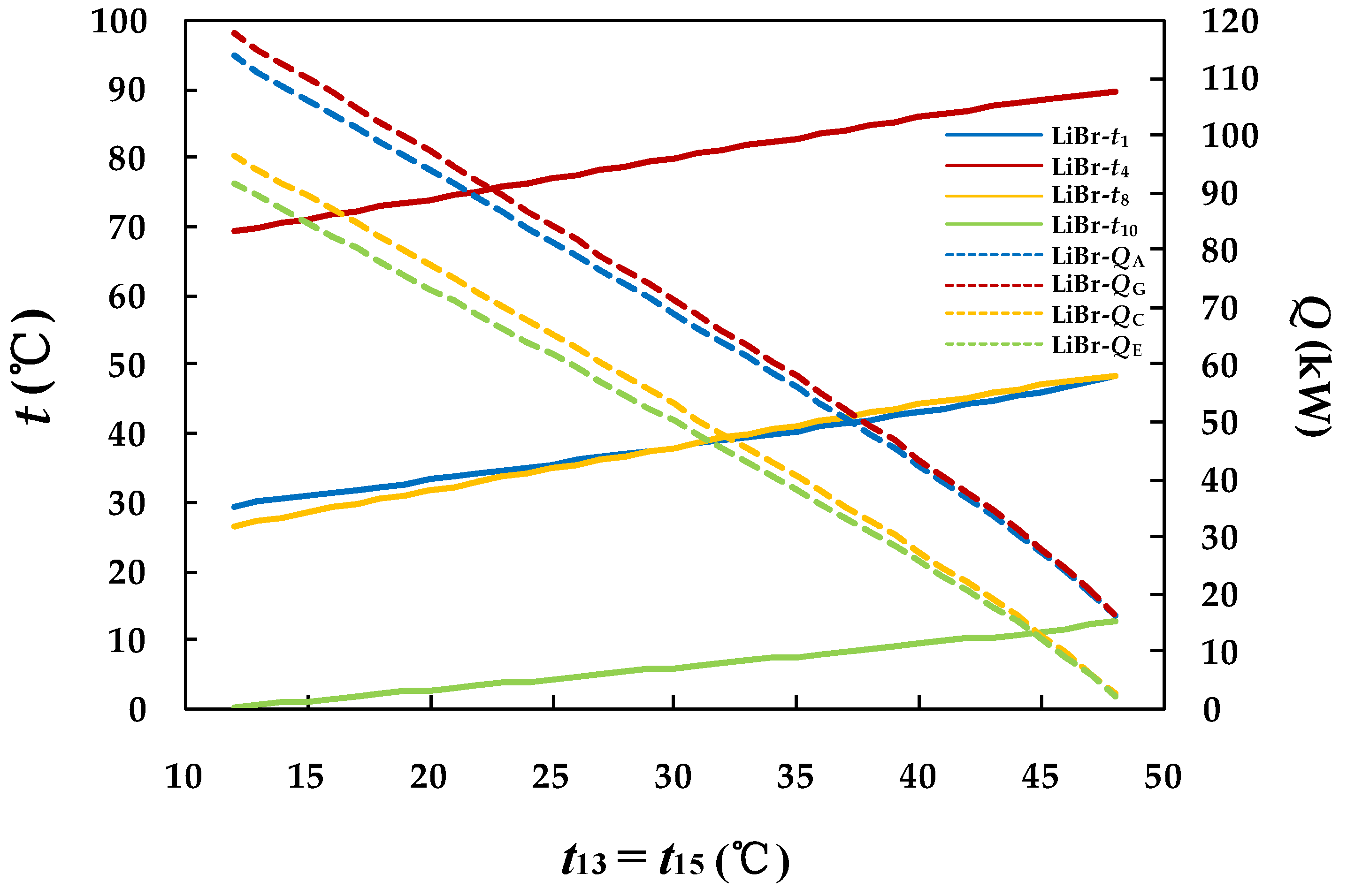
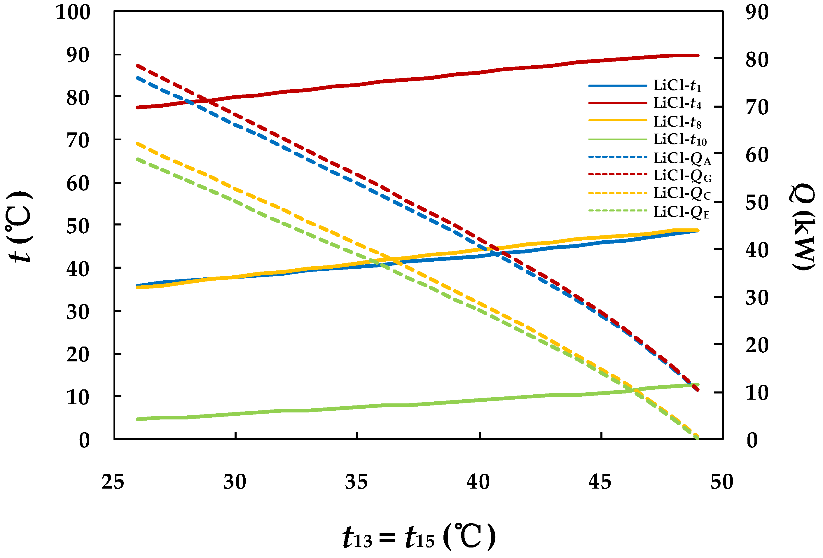
4.3.2. Effect of Cooling Water Inlet Temperature in Absorber and Condenser

It can be ascertained from Figure 16 that cooling water between the condenser and absorber severely affected the performance of both absorption chillers. The LiCl-H₂O system could not operate at a lower cooling temperature than 26 °C. The COP and exergetic efficiency displayed an initial steady degression, but plummeted when the inlet temperature of the cooling water passed 41 °C. This was mainly because the cooling capacity slipped to a smaller value and descended quickly compared to the heat input at the generator as the inlet temperature rose. In the meantime, it can be observed from Figure 17 and Figure 18 that the temperatures of components all displayed an upward trend while the heat duties of all components were completely the opposite. The reason will be explained as follows.

In the first place, the working conditions of the absorber and condenser were directly affected by the inlet temperature of the cooling water. On the one hand, the weak solution temperature of the absorber increased with the inlet cooling water temperature increasing, which led to the increase of the mass fraction of the weak solution. On the other hand, the condensation temperature went up due to the enhanced heat transfer with the cooling water, and also the corresponding condensation pressure, causing a reduction of the strong solution concentration. As a result, the circulation ratio of the solution increased while the mass flow rate of the solution pump remained constant, resulting in the reduction of the refrigerant quantity and eventually the condensing and cooling capacity decreased. Consequently, the heat duties of the generator and absorber declined due to a lower solution circulation ratio; therefore, the temperature difference between the inlet and outlet temperature of the external circuit water decreased under the condition that mass flow rates were unchanged.

The rate of decrease in the cooling capacity was within 10% for the LiBr-H₂O system with cooling water temperatures between 12 °C and 41 °C in comparison to the LiCl-H₂O system between 26 °C and 41 °C; otherwise, the rate dropped dramatically above this range and even more than 40% at the highest temperatures.

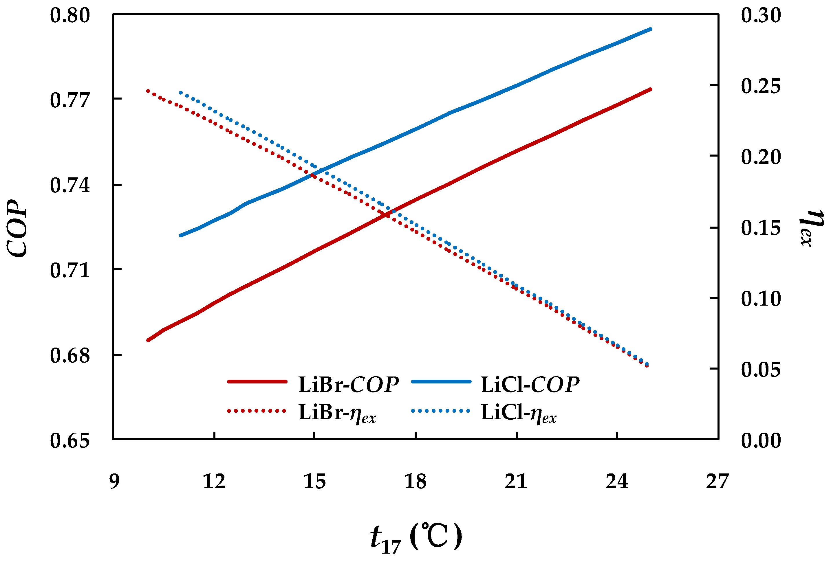
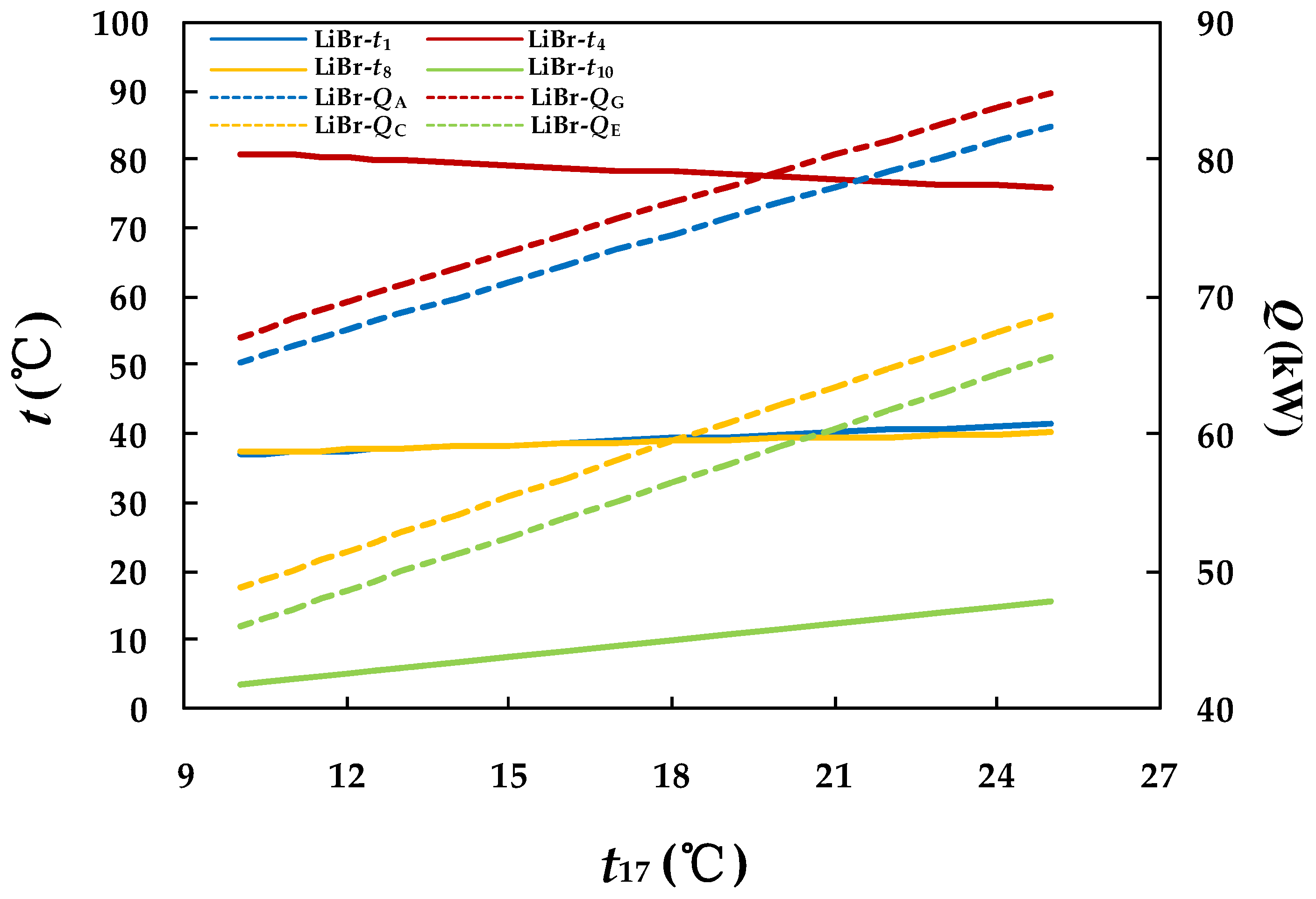
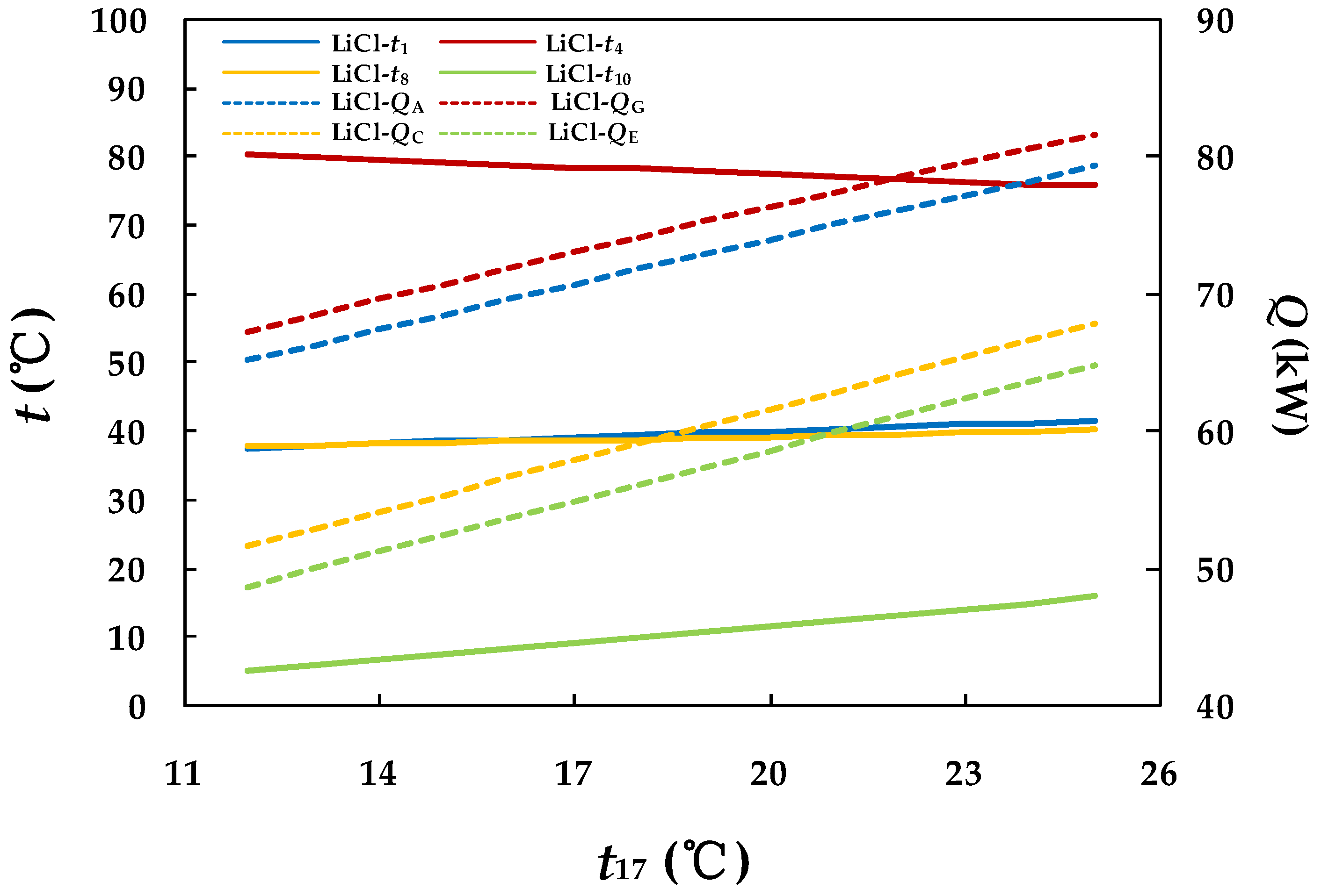
4.3.3. Effect of Chilled Water Inlet Temperature in Evaporator

The effects of the inlet temperature of chilled water in the evaporator on the performance of both absorption chillers are illustrated in Figure 19, Figure 20 and Figure 21. It can be seen that the COP and heat capacities of all the components present a linear growth, as well as the evaporator temperature, which is exactly contrary to the tendency of the exergetic efficiency and the solution temperature at the exit of the generator. Likewise, the temperatures of the absorber and condenser were much the same for both systems and increased slightly with the inlet temperature of chilled water, which were a little higher for the absorber temperature.

In order to explain them, the effect of the chilled water on the evaporator should be investigated first. It was not difficult to find that the evaporation temperature increased with the inlet temperature of chilled water for considering the evaporator as a heat exchanger when the average temperature of the hot-fluid side rose under the constant mass flow rate and heat transfer characteristic. Therefore, the evaporation pressure increased along with the absorption pressure, which promoted the ability of the vapor absorption of a strong solution in the absorber, consequently reducing the mass fraction of the weak solution. In addition, the condensation temperature showed an upward trend with the chilled water inlet temperature rising, which resulted in the mass fraction of the strong solution decreasing because of the decline in the generator temperature and restriction of the Dühring rule in Equation (10). However, the concentration decrement of the strong solution was less than the weak solution, which caused the deflation ratio of the chiller to increase and the solution circulation ratio to decrease, therefore producing a greater quantity of refrigerant vapor in a cycle. This was the reason for the increase in the condenser and evaporator heat loads. For the absorber and generator, to generate the vapor or absorb the refrigerant accompanied with the phase change involved a considerable heat transfer in the process that was more than the same amount of liquid solution. Thus, an increasing of refrigerant quantity yielded to the heat loads in the absorber and generator augment as the mass flow rate of the solution pump remained constant.

Unlike the previous situations, in this case, the temperatures of the solution exiting from the absorber and generator presented an opposite trend according to the calculations, which showed an upward trend for the former and downward for the latter. The reason was that the temperatures of weak and strong solutions were closely related to the heat capacities of the absorber and generator, which mainly depended on the solution circulation ratio, but more importantly, the specific mass flow rate of each state point played a crucial role.

In both circumstances, the increased rate in cooling capacity was about 2–3% °C⁻¹ with the inlet temperature of chilled water rising and ranged between 10 °C and 25 °C for the LiBr-H₂O system in comparison to the LiCl-H₂O system between 12 °C and 25 °C. The COP increased from 0.68 to 0.77 for the LiBr-H₂O system and from 0.72 to 0.79 for the LiCl-H₂O system, whereas the exergetic efficiency of both chillers presented a downward trend with an increasing decrement in the range of ≈5–22% °C⁻¹. In addition, the COP or exergetic efficiency gap between the two chillers shrunk.

In this section, the effects of a single change in the inlet temperature of the external circuit flows have been researched. From all of the above calculation results, something in common can be observed, which is that the temperatures of the fluid exiting from components of two chillers were almost the same as each other. This shows that the difference of heat duties in the same component of two chillers was mainly up to the thermodynamic properties of the solution, especially for the generator and absorber. That is why the LiCl-H₂O was superior to LiBr-H₂O in performance, but limited in application.

5. Conclusions

In this study, the use of LiBr-H₂O and LiCl-H₂O working pairs in the absorption refrigeration system were investigated from two aspects with multiple evaluation criteria. First, a novel calculation model was developed to investigate the performance of a single effect ARS and the model was validated with the available data in the literature. The effect of various design parameters was examined using energy and efficiency analyses. Second, the LiBr-H₂O and LiCl-H₂O absorption chillers with a capacity of 50 kW were designed with the same parameters. Then, the computer program of the absorption chiller was established to examine its performance under off-design external temperature conditions based on energy and exergy analysis. The main conclusions that can be drawn are as follows.

The COP and efficiency ratio in both systems increased with the generator temperature when the condenser and absorber temperatures were kept constant, but further increases brought down the efficiency ratio instead of being straight and level as for the COP. Lower temperatures of the condenser and absorber led to a higher COP and efficiency ratio, as well as their maximum values, consequently reducing the optimum generator temperature. The COP of both systems increased with evaporator temperature, but the growth rate weakened and all the values approached 0.8 eventually.

The variation of the generator temperature was limited as an upper bound by condenser temperature for the strong solution crystallization after the solution heat exchanger. The lowest generator temperature of the weak solution was decided by the absorber and evaporator temperatures. As a consequence, for better performance, a higher condensation or absorption temperature is more appropriate with a higher generator temperature, and vice versa for a lower evaporator temperature.

The studies on off-design conditions indicate that the inlet temperature of hot water with an optimum COP of the chiller was about 98 °C and 83 °C for LiBr-H₂O and LiCl-H₂O, respectively. However, the exergetic efficiency of the absorption chiller was negatively affected by the increase of the heat source temperature. In addition, the influences of the cooling water inlet temperature between the condenser and absorber on the performance were remarkable for both absorption chillers. The COP and exergetic efficiency degraded dramatically when the cooling water temperature was over the 41 °C for both chillers. With the inlet temperature of the chilled water rising, the cooling capacity of both chillers increased with the rate about 2–3% °C⁻¹ and the COP also increased, but this was opposite to the case of the exergetic efficiency.

The final conclusion of this study is that the LiCl-H₂O system has great limitations for practical application due to the crystallization problem though it performed better than a conventional LiBr-H₂O system under identical operating conditions. Compared to the LiBr-H₂O system, a LiCl-H₂O system is more appropriate for the situation where it is provided with a somewhat lower generator temperature or higher condenser temperature. After all, the diversity performances of the two working pairs depended on their own thermodynamic properties.

References

1. Ebrahimi, K.; Jones, G.F.; Fleischer, A.S. A review of data center cooling technology, operating conditions and the corresponding low-grade waste heat recovery opportunities. Renew. Sustain. Energy Rev. 2014, 31, 622–638. [Google Scholar] [CrossRef]
2. Mbikan, M.; Al-Shemmeri, T. Computational Model of a Biomass Driven Absorption Refrigeration System. Energies 2017, 10, 234. [Google Scholar] [CrossRef]
3. Alobaid, M.; Hughes, B.; Calautit, J.K.; O’Connor, D.; Heyes, A. A review of solar driven absorption cooling with photovoltaic thermal systems. Renew. Sustain. Energy Rev. 2017, 76, 728–742. [Google Scholar] [CrossRef] [Green Version]
4. Mahmoudi, S.; Kordlar, M.A. A new flexible geothermal based cogeneration system producing power and refrigeration. Renew. Energy 2018, 123, 499–512. [Google Scholar] [CrossRef]
5. Srikhirin, P.; Aphornratana, S.; Chungpaibulpatana, S. A review of absorption refrigeration technologies. Renew. Sustain. Energy Rev. 2001, 5, 343–372. [Google Scholar] [CrossRef]
6. Sun, J.; Fu, L.; Zhang, S. A review of working fluids of absorption cycles. Renew. Sustain. Energy Rev. 2012, 16, 1899–1906. [Google Scholar] [CrossRef]
7. Wang, J.; Yan, Z.; Wang, M.; Dai, Y. Thermodynamic analysis and optimization of an ammonia-water power system with LNG (liquefied natural gas) as its heat sink. Energy 2013, 50, 513–522. [Google Scholar] [CrossRef]
8. Günhan, T.; Ekren, O.; Demir, V.; Hepbasli, A.; Erek, A.; Şahin, A. Şencan Experimental exergetic performance evaluation of a novel solar assisted LiCl–H2O absorption cooling system. Energy Build. 2014, 68, 138–146. [Google Scholar] [CrossRef]
9. Moreno-Quintanar, G.; Rivera, W.; Best, R. Comparison of the experimental evaluation of a solar intermittent refrigeration system for ice production operating with the mixtures NH3/LiNO3 and NH3/LiNO3/H2O. Renew. Energy 2012, 38, 62–68. [Google Scholar] [CrossRef]
10. Cai, D.H.; Jiang, J.K.; He, G.G.; Li, K.Q.; Niu, L.J.; Xiao, R.X. Experimental evaluation on thermal performance of an air-cooled absorption refrigeration cycle with NH3-LiNO3 and NH3-NaSCN refrigerant solutions. Energy Conv. Manag. 2016, 120, 32–43. [Google Scholar] [CrossRef]
11. Asfand, F.; Stiriba, Y.; Bourouis, M. Performance evaluation of membrane-based absorbers employing H2O/(LiBr + LiI + LiNO3 + LiCl) and H2O/(LiNO3+KNO3+NaNO3) as working pairs in absorption cooling systems. Energy 2016, 115, 781–790. [Google Scholar] [CrossRef]
12. Alvarez, M.E.; Esteve, X.; Bourouis, M. Performance analysis of a triple-effect absorption cooling cycle using aqueous (lithium, potassium, sodium) nitrate solution as a working pair. Appl. Therm. Eng. 2015, 79, 27–36. [Google Scholar] [CrossRef]
13. Gommed, K.; Grossman, G.; Ziegler, F. Experimental Investigation of a LiCl-Water Open Absorption System for Cooling and Dehumidification. J. Sol. Energy Eng. 2004, 126, 710–715. [Google Scholar] [CrossRef]
14. Conde, M.R. Properties of aqueous solutions of lithium and calcium chlorides: Formulations for use in air conditioning equipment design. Int. J. Therm. Sci. 2004, 43, 367–382. [Google Scholar] [CrossRef]
15. Kim, D.; Ferreira, C.I. A Gibbs energy equation for LiBr aqueous solutions. Int. J. Refrig. 2006, 29, 36–46. [Google Scholar] [CrossRef]
16. Pátek, J.; Klomfar, J. Solid–liquid phase equilibrium in the systems of LiBr–H2O and LiCl–H2O. Fluid Phase Equilibria 2006, 250, 138–149. [Google Scholar] [CrossRef]
17. Pátek, J.; Klomfar, J. A computationally effective formulation of the thermodynamic properties of LiBr–H2O solutions from 273 to 500K over full composition range. Int. J. Refrig. 2006, 29, 566–578. [Google Scholar] [CrossRef]
18. Pátek, J.; Klomfar, J. Thermodynamic properties of the LiCl–H2O system at vapor–liquid equilibrium from 273 K to 400 K. Int. J. Refrig. 2008, 31, 287–303. [Google Scholar] [CrossRef]
19. Parham, K.; Atikol, U.; Yari, M.; Agboola, O.P. Evaluation and optimization of single stage absorption chiller using (LiCl+H2O) as the working pair. Adv. Mech. Eng. 2013, 2013. [Google Scholar] [CrossRef]
20. Patel, J.; Pandya, B.; Mudgal, A. Exergy Based Analysis of LiCl-H2O Absorption Cooling System. Energy Procedia 2017, 109, 261–269. [Google Scholar] [CrossRef]
21. Bellos, E.; Tzivanidis, C.; Antonopoulos, K.A. Exergetic and energetic comparison of LiCl-H2O and LiBr-H2O working pairs in a solar absorption cooling system. Energy Convers. Manag. 2016, 123, 453–461. [Google Scholar] [CrossRef]
22. Gogoi, T.; Konwar, D. Exergy analysis of a H2O–LiCl absorption refrigeration system with operating temperatures estimated through inverse analysis. Energy Convers. Manag. 2016, 110, 436–447. [Google Scholar] [CrossRef]
23. She, X.H.; Yin, Y.G.; Xu, M.F.; Zhang, X.S. A novel low-grade heat-driven absorption refrigeration system with LiCl-H2O and LiBr-H2O working pairs. Int. J. Refrig. 2015, 58, 219–234. [Google Scholar] [CrossRef]
24. Ochoa, A.; Dutra, J.; Henríquez, J.; Dos Santos, C. Dynamic study of a single effect absorption chiller using the pair LiBr/H2O. Energy Convers. Manag. 2016, 108, 30–42. [Google Scholar] [CrossRef]
25. Ochoa, A.; Dutra, J.; Henríquez, J.; Dos Santos, C.; Rohatgi, J. The influence of the overall heat transfer coefficients in the dynamic behavior of a single effect absorption chiller using the pair LiBr/H2O. Energy Convers. Manag. 2017, 136, 270–282. [Google Scholar] [CrossRef]
26. Marc, O.; Sinama, F.; Praene, J.-P.; Lucas, F.; Castaing-Lasvignottes, J. Dynamic modeling and experimental validation elements of a 30 kW LiBr/H2O single effect absorption chiller for solar application. Appl. Therm. Eng. 2015, 90, 980–993. [Google Scholar] [CrossRef]
27. Kohlenbach, P.; Ziegler, F. A dynamic simulation model for transient absorption chiller performance. Part I: The model. Int. J. Refrig. 2008, 31, 217–225. [Google Scholar] [CrossRef]
28. Kohlenbach, P.; Ziegler, F. A dynamic simulation model for transient absorption chiller performance. Part II: Numerical results and experimental verification. Int. J. Refrig. 2008, 31, 226–233. [Google Scholar] [CrossRef]
29. Hellmann, H.M.; Schweigler, C.; Ziegler, F. A Simple Method for Modelling the Operating Characteristics of Absorption Chillers. In Proceedings of the Thermodynamics Heat and Mass Transfers of Refrigeration Machines and Heat Pumps Seminar Eurotherm No. 59, Nancy, France, 6–7 July 1998; pp. 219–226. [Google Scholar]
30. Arnavat, M.P.; López-Villada, J.; Bruno, J.C.; Coronas, A. Analysis and parameter identification for characteristic equations of single- and double-effect absorption chillers by means of multivariable regression. Int. J. Refrig. 2010, 33, 70–78. [Google Scholar] [CrossRef]
31. Gutiérrez-Urueta, G.; Rodríguez, P.; Ziegler, F.; Lecuona, A.; Rodríguez-Hidalgo, M. Extension of the characteristic equation to absorption chillers with adiabatic absorbers. Int. J. Refrig. 2012, 35, 709–718. [Google Scholar] [CrossRef] [Green Version]
32. Kim, D.; Ferreira, C.I. Analytic modelling of steady state single-effect absorption cycles. Int. J. Refrig. 2008, 31, 1012–1020. [Google Scholar] [CrossRef]
33. Wagner, W.; Cooper, J.R.; Dittmann, A.; Kijima, J.; Kretzschmar, H.J.; Kruse, A.; Mareš, R.; Oguchi, K.; Sato, H.; Stöcker, I.; et al. The IAPWS Industrial Formulation 1997 for the Thermodynamic Properties of Water and Steam. J. Eng. Gas Turbines Power 2000, 122, 150–184. [Google Scholar] [CrossRef]
34. Patel, H.A.; Patel, L.; Jani, D.; Christian, A. Energetic Analysis of Single Stage Lithium Bromide Water Absorption Refrigeration System. Procedia Technol. 2016, 23, 488–495. [Google Scholar] [CrossRef] [Green Version]
35. Edgar, T.F.; Himmelblau, D.M.; Lasdon, L.S. Optimization of Chemical Processes; McGraw-Hill: New York, NY, USA, 2001. [Google Scholar]
36. Gebreslassie, B.H.; Groll, E.A.; Garimella, S.V. Multi-objective optimization of sustainable single-effect water/Lithium Bromide absorption cycle. Renew. Energy 2012, 46, 100–110. [Google Scholar] [CrossRef] [Green Version]
37. Martínez, J.C.; Martinez, P.; Bujedo, L.A. Development and experimental validation of a simulation model to reproduce the performance of a 17.6 kW LiBr–water absorption chiller. Renew. Energy 2016, 86, 473–482. [Google Scholar] [CrossRef]
38. Kerme, E.D.; Chafidz, A.; Agboola, O.P.; Orfi, J.; Fakeeha, A.H.; Al-Fatesh, A.S. Energetic and exergetic analysis of solar-powered lithium bromide-water absorption cooling system. J. Clean. Prod. 2017, 151, 60–73. [Google Scholar] [CrossRef]
39. Kaita, Y. Simulation results of triple-effect absorption cycles. Int. J. Refrig. 2002, 25, 999–1007. [Google Scholar] [CrossRef]
40. Anand, D.; Kumar, B. Absorption machine irreversibility using new entropy calculations. Sol. Energy 1987, 39, 243–256. [Google Scholar] [CrossRef]
41. Kaushik, S.; Arora, A. Energy and exergy analysis of single effect and series flow double effect water–lithium bromide absorption refrigeration systems. Int. J. Refrig. 2009, 32, 1247–1258. [Google Scholar] [CrossRef]
Figure 1. (a) Schematic representation of the single effect absorption refrigeration system, and (b) the pressure–temperature (P–T) diagram of the cycle.
Energies 12 03037 g001
Figure 2. Flow chart of the calculation procedure.
Energies 12 03037 g002
Figure 3. Generator temperature impact on the COP of the absorption system under various condenser and absorber temperature levels (32 °C, 36 °C, and 40 °C) for the two working pairs (t10 = 7 °C, ε = 0.7).
Energies 12 03037 g003
Figure 4. Generator temperature impact on the efficiency ratio of absorption system under various condenser and absorber temperature levels (32 °C, 36 °C, and 40 °C) for the two working pairs (t10 = 7 °C, ε = 0.7).
Energies 12 03037 g004
Figure 5. Condenser and absorber temperatures impact on the COP of the absorption system under various generator temperature levels (78 °C, 80 °C, and 82 °C) for the two working pairs (t10 = 7 °C, ε = 0.7).
Energies 12 03037 g005
Figure 6. Condenser and absorber temperatures impact on the efficiency ratio of the absorption system under various generator temperature levels (78 °C, 80 °C, and 82 °C) for the two working pairs (t10 = 7 °C, ε = 0.7).
Energies 12 03037 g006
Figure 7. Absorber temperature impact on the COP and efficiency ratio of the absorption system under the examined operating condition for the two working pairs (t4 = 80 °C, t8 = 40 °C, t10 = 7 °C, ε = 0.7).
Energies 12 03037 g007
Figure 8. Condenser temperature impact on the COP and efficiency ratio of absorption system under the examined operating condition for the two working pairs (t1 = 40 °C, t4 = 80 °C, t10 = 7 °C, ε = 0.7).
Energies 12 03037 g008
Figure 9. Evaporator temperature impact on the COP of the absorption system under various generator temperature levels (78 °C, 80 °C, and 82 °C) for the two working pairs (t1 = t8 = 40 °C, ε = 0.7).
Energies 12 03037 g009
Figure 10. Evaporator temperature impact on the efficiency ratio of absorption system under various generator temperature levels (78 °C, 80 °C, and 82 °C) for the two working pairs (t1 = t8 = 40 °C, ε = 0.7).
Energies 12 03037 g010
Figure 11. Heat exchanger effectiveness impact on the COP of the absorption system under various generator temperature levels (78 °C, 80 °C, and 82 °C) for the two working pairs (t1 = t8 = 40 °C, t10 = 7 °C, ε = 0.7).
Energies 12 03037 g011
Figure 12. Heat exchanger effectiveness impact on the efficiency ratio of the absorption system under various generator temperature levels (78 °C, 80 °C, and 82 °C) for the two working pairs (t1 = t8 = 40 °C, t10 = 7 °C, ε = 0.7).
Energies 12 03037 g012
Figure 13. Variation of COP and exergy efficiency with the hot water inlet temperature for the two absorption chillers.
Energies 12 03037 g013
Figure 14. Variations of the exit temperatures of the internal and external fluids with hot water inlet temperature for the LiBr-H2O absorption chiller.
Energies 12 03037 g014
Figure 15. Variations of the exit temperatures of the internal and external fluids with hot water inlet temperature for the LiCl-H2O absorption chiller.
Energies 12 03037 g015
Figure 16. Variation of COP and the exergy efficiency with the cooling water inlet temperature for the two absorption chillers.
Energies 12 03037 g016
Figure 17. Variation of the exit temperature and heat capacity of each component with the cooling water inlet temperature for the LiBr-H2O absorption chiller.
Energies 12 03037 g017
Figure 18. Variation of the exit temperature and heat capacity of each component with the cooling water inlet temperature for LiCl-H2O absorption chiller.
Energies 12 03037 g018
Figure 19. Variation of COP and exergy efficiency with the chilled water inlet temperature for the two absorption chillers.
Energies 12 03037 g019
Figure 20. Variation of the exit temperature and heat capacity of each component with the chilled water inlet temperature for the LiBr-H2O absorption chiller.
Energies 12 03037 g020
Figure 21. Variation of the exit temperature and heat capacity of each component with the cooling water inlet temperature for the LiCl-H2O absorption chiller.
Energies 12 03037 g021