Empirical Conductivity Equation for the Simulation of the Stationary Space Charge Distribution in Polymeric HVDC Cable Insulations ^†

Abstract

Many processes are involved in the accumulation of space charges within the insulation materials of high voltage direct current (HVDC) cables, e.g., the local electric field, a conductivity gradient inside the insulation, and the injection of charges at both electrodes. An accurate description of the time dependent charge distribution needs to include these effects. Furthermore, using an explicit Euler method for the time integration of a suitably formulated transient model, low time steps are used to resolve fast charge dynamics and to satisfy the Courant–Friedrichs–Lewy (CFL) stability condition. The long lifetime of power cables makes the use of a final stationary charge distribution necessary to assess the reliability of the cable insulations. For an accurate description of the stationary space charge and electric field distribution, an empirical conductivity equation is developed. The bulk conductivity, found in literature, is extended with two sigmoid functions to represent a conductivity gradient near the electrodes. With this extended conductivity equation, accumulated bulk space charges and hetero charges are simulated. New introduced constants to specify the sigmoid functions are determined by space charge measurements, taken from the literature. The measurements indicate accumulated hetero charges in about one quarter of the insulation thickness in the vicinity of both electrodes. The simulation results conform well to published measurements and show an improvement to previously published models, i.e., the developed model shows a good approximation to simulate the stationary bulk and hetero charge distribution.

1. Introduction

The charge transportation behavior and accumulation in high voltage direct current (HVDC) cable insulations result in reliability problems of these components, due to an increased local electric field strength. In comparison to measurements, a cheap alternative is the simulation of such a charge distribution, using a conductivity model for the insulation. Typical conductivity models show a dependency on the electric field and the temperature [1]. For an accurate description of the space charge density, conductivity models need to include different effects. Short term effects are injection and extraction processes at both electrodes and charge packets. Relatively long term effects are the accumulation of bulk charges within the insulation and the presence of homo or hetero charges in the vicinity of both electrodes. Due to the long operation time of direct current (DC) power cables that are in service from several years up to decades, only long term effects are considered and the stationary charge distribution is simulated to determine the reliability of the insulation material.

Commonly used cable insulation materials are cross-linked polyethylene (XLPE) and low-density polyethylene (LDPE). These materials are in use due to their good electrical characteristics, ease of processing, and acceptable cost [1,2].

Depending on the charge type, high electric fields occur inside the insulation or in the vicinity of the electrodes. At low electric fields, the charge movement is higher than the charge injection. The injected charges move across the insulation, resulting in accumulated hetero charges and an increased electric field at both electrodes. At high electric fields, the charge movement is less than the charge injection and homo charges accumulate, resulting in decreased electric fields at the electrodes and increased electric fields within the insulation bulk [3,4].

Typically, the insulation material in power cables contains a semiconducting layer at the anode and another one at the cathode. Moving injected charges are blocked at these layers and form hetero charges. Furthermore, with an applied electric field, ionized impurities move towards the electrodes and form hetero charges as well. The electric field of the applied voltage is superimposed by the electric field of the hetero charges. As a consequence, the resulting electric field stress can exceed the breakdown strength of the insulation [5].

Without an applied temperature gradient, most of the charges accumulate in the vicinity of the electrodes. With an applied temperature gradient, bulk space charges accumulate, where the magnitude increases with increasing temperature gradient and, thus, with increasing conductivity gradient.

Accumulated space charges, either homo or hetero charges, result from different sources, e.g., the electrode material, the applied temperature gradient, or the local electric field. Due to common applied electric fields of less than 20 kV/mm within polymeric cable insulations (see [4]) and measured hetero charges in XLPE and LDPE insulations at an average electric field below 20 kV/mm, only the accumulation of hetero charges is considered in the simulations [6,7].

Typical conductivity-based cable models show a dependency on the electric field and the temperature. Thus, only bulk space charges are simulated and charges in the vicinity of the electrodes are neglected. Due to many processes (e.g., injection and extraction of charges at the electrodes), it is difficult to predict accumulated charges in the vicinity of the electrodes. In some cases, charges at the electrodes are higher compared to bulk space charges (see Figures 4a and 5). Thus, the resulting electric field is also increased, considering charges at the electrodes and common conductivity models that neglect homo or hetero charges are less reliable [4].

In [8], a conductivity model is used to predict the time dependent charge behavior. Inside XLPE insulation materials, a varying conductivity and permittivity in the vicinity of electrodes is discussed in [9]. In this paper, the stationary charge distribution in polymeric cable insulations is simulated, using an improved conductivity model. To validate the developed model and to find a general expression for the bulk and hetero space density in polymeric cable insulations, space charge measurements, taken from literature, are used.

The next section is about the development of an empirical conductivity model equation and the basic equations to simulate the stationary charge distribution. The simulation results are discussed and are compared against measurements in the third section. The obtained results are concluded in a short summary in section IV.

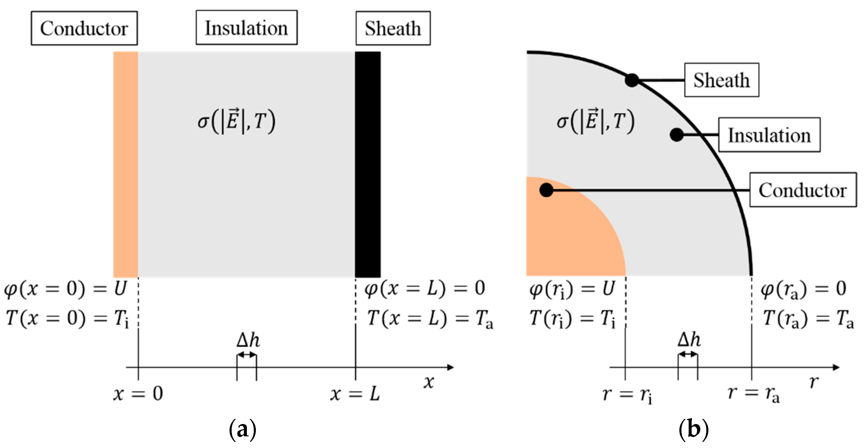
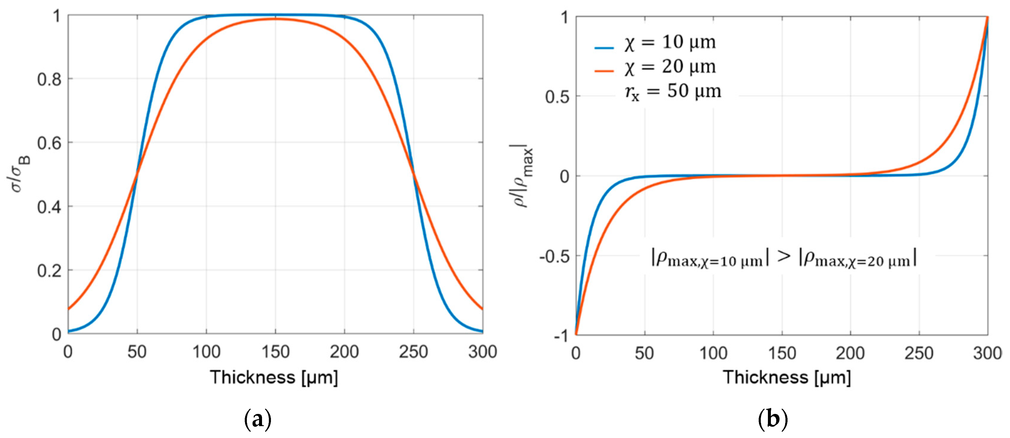
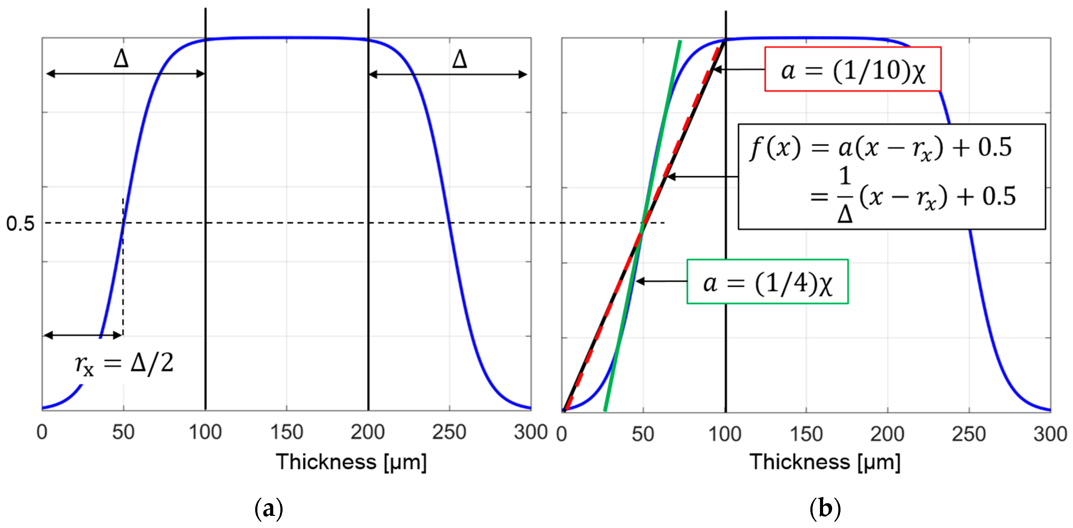
2. Empirical Conductivity Model Equation for the Simulation of the Stationary Charge Distribution

The stationary space charge and electric field distribution is computed, using the system of partial differential equations consisting of the stationary continuity equation, Poisson’s equation, and Ohm’s law, i.e.,

$$\mathrm{div}\hspace{0.17em}\overrightarrow{J}=0,$$

(1)

$$\mathrm{div}\left(\epsilon \hspace{0.17em}\mathrm{grad}\hspace{0.17em}\phi \right)=-\rho ,$$

(2)

$$\overrightarrow{J}=\sigma \overrightarrow{E},$$

(3)

where $\overrightarrow{J}$ is the current density inside the insulation, $\overrightarrow{E}=-\mathrm{grad}\hspace{0.17em}\phi$ is the magnitude of the electric field, φ is the electric potential, ρ is the space charge density, σ is the electric conductivity, ε = ε₀ε_r, where ε₀ = 8.854 × 10⁻¹² As/(Vm) is the dielectric constant and ε_r is the relative permittivity [9]. The Equations (1)–(3) are solved using the finite-difference method in one dimension. Depending on the geometry, depicted in Figure 1, a uniform grid of spacing Δh in either radial direction or x-direction is utilized, respectively [10]. Simulation results of a 150 μm thick insulating material are given in [11], where a non-uniform grid of minimum nodal distance 0.1 μm is used. To provide a sufficiently accurate spatial discretization for both geometries in Figure 1, the distance between the anode and the cathode is discretized with N = 1500 equidistant grid points in this work.

The thickness of the planplanar insulation is L, the radius of the inner cable conductor is r_i, the radius of the outer sheath is r_a, the conductor temperature is T_i, the sheath temperature is T_a, and the applied voltage is U.

In literature, the conductivity of polymeric insulations is typically modeled with an Arrhenius-type conductivity-temperature relationship. The electric field shows a dependency with a “sinh” (see e.g., [12,13]). The bulk conductivity σ_B of polymeric insulations is given by

$${\sigma }_{\mathrm{B}}=(|\overrightarrow{J_0}|/|\overrightarrow{E}|)\exp (-E_{\mathrm{a}}/(kT))\sinh (\gamma |\overrightarrow{E}|),$$

(4)

where k = 1.38 × 10⁻²³ J/K is the Boltzmann constant, T is the temperature, $|J_0|$ is a current density constant, E_a is the activation energy, and γ is a constant to describe the dependency on the electric field [13]. These constants are determined by a fit of Equation (4) to measured data. The constants of XLPE insulations are approximately $|J_0|$ = 1 × 10¹⁴ A/m², E_a = 1.48 eV and γ = 2 × 10⁻⁷ m/V (see [13]). For an LDPE insulation, the constants are $|J_0|$ = 0.04224 A/m², E_a = 0.84 eV and γ = 4.251 × 10⁻⁷ m/V (see [14,15,16]).

Analogously to [9], hetero charge accumulation in the vicinity of both electrodes is described by a conductivity gradient with two sigmoid functions. The total electric conductivity σ inside a cylindrical insulation is modeled by

$$\sigma ={\sigma }_B\left(K_1-K_2\right),$$

(5)

$$K_1=\frac{1}{1+\exp \left(-\frac{r-r_{\mathrm{i}}-r_{\mathrm{x}}}{\chi }\right)},$$

(6)

$$K_2=\frac{1}{1+\exp \left(-\frac{r-r_{\mathrm{a}}+r_{\mathrm{x}}}{\chi }\right)},$$

(7)

where K₁ describes the conductivity variations at the inner conductor (anode) and K₂ the conductivity variations at the outer sheath (cathode); in (6) and (7), r_x is the distance between r_i and the position of the highest gradient (σ/σ_B(r = r_x) = 0.5). If a planplanar insulation is considered, r → x, r_i = 0 and r_a = L holds.

The distance constant χ defines the conductivity gradient in the vicinity of both electrodes (see Figure 2a), which affects the magnitude and the shape of the hetero charges distribution (see Figure 2b). For example, in Figure 2 χ = 10 μm and χ = 20 μm with r_x = 50 μm are depicted. Increasing the distance constant χ results in a decreasing conductivity gradient and hetero charges distribution, with a slightly spread out charge shape. In Figure 2, a constant bulk conductivity (σ_B = const.) is used for the computation of the stationary space charge density ρ [10].

A conductivity increase is described with K₁, resulting in negative charges at the anode and K₂ is describing a conductivity decrease, resulting in positive charges at the cathode. This relationship is obtained from the analytic solution of the stationary charge and electric field distribution, using a conductivity gradient.

Assuming a spatial varying conductivity σ(r) = σ₀ × K₁, where σ₀ is a constant conductivity, and a planplanar insulation (see Figure 1a). Using (1), (3), and Gauss law, the stationary charge density is computed by

$$\mathrm{div}(\epsilon \overrightarrow{E})=\mathrm{div}\left(\epsilon \frac{\overrightarrow{J}}{\sigma }\right)=\frac{\epsilon }{\sigma }\mathrm{div}\left(\overrightarrow{J}\right)+\overrightarrow{J}\mathrm{grad}\left(\frac{\epsilon }{\sigma }\right)=\sigma \overrightarrow{E}\hspace{0.17em}\mathrm{grad}\left(\frac{\epsilon }{\sigma }\right)=\rho .$$

(8)

With (2) and $\overrightarrow{E}=-\mathrm{grad}\hspace{0.17em}\phi$, the stationary electric field within a homogeneous (ε_r = constant) insulation is computed by

$$\epsilon \frac{\partial }{\partial x}E(x)=\epsilon \sigma E(x)\hspace{0.17em}\frac{\partial }{\partial x}\left(\frac{1}{\sigma }\right).$$

(9)

To obtain the stationary electric field, the solution of

$$\frac{\partial }{\partial x}E(x)-E(x)\left[\sigma \frac{\partial }{\partial x}\frac{1}{\sigma }\right]=0$$

(10)

is given by

$$E_{\mathrm{an}}(x)=C\cdot \exp \left(\ln \left\{1+\exp \left(-\frac{x-r_{\mathrm{x}}}{\chi }\right)\right\}\right)=C\cdot \left\{1+\exp \left(-\frac{x-r_{\mathrm{x}}}{\chi }\right)\right\},$$

(11)

where C is a constant, that is computed by

$$U={\displaystyle \underset{0}{\overset{L}{\int }}E(x)dx}\to C=\frac{U}{{\displaystyle \underset{0}{\overset{L}{\int }}1+\exp \left(-\frac{x-r_{\mathrm{x}}}{\chi }\right)dx}}=\frac{U}{L+\chi \exp \left(\frac{r_{\mathrm{x}}}{\chi }\right)-\chi \exp \left(-\frac{L-r_{\mathrm{x}}}{\chi }\right)}.$$

(12)

Measurements indicate hetero charges located near the electrodes and less charges are within the bulk. Thus, the conductivity gradient is also located near the electrodes and L $\gg$ r_x. With L $\gg$ r_x, the constant C is positive. With (11) and Gauss law, the stationary charge density is given by

$${\rho }_{\mathrm{an}}(x)=\frac{\partial }{\partial x}(\epsilon E(x))=-\frac{1}{\chi }\epsilon \hspace{0.17em}C\exp \left(-\frac{x-r_{\mathrm{x}}}{\chi }\right).$$

(13)

From (13), we see that the conductivity increases results in negative charges. Using a decreasing conductivity σ(r) = σ₀ × (1 − K₂) positive charges are modeled at the sheath, where the computation is analog to (8)–(10). The electric field is

$$E_{\mathrm{ca}}(x)=C\cdot \exp \left(\ln \left\{1+\exp \left(\frac{x-L_{\mathrm{a}}+r_{\mathrm{x}}}{\chi }\right)\right\}\right)=C\cdot \left\{1+\exp \left(\frac{x-L+r_{\mathrm{x}}}{\chi }\right)\right\},$$

(14)

where C is equal to (12). The stationary charge density is

$${\rho }_{\mathrm{ca}}(x)=\frac{\partial }{\partial x}(\epsilon E(x))=\frac{1}{\chi }\epsilon \hspace{0.17em}C\exp \left(\frac{x-L+r_{\mathrm{x}}}{\chi }\right).$$

(15)

To determine the constants r_x and χ, the region of the conductivity gradient is defined by Δ. In Figure 3, (6) and (7) are depicted for a planplanar geometry [10]. To determine the dependency of r_x and χ on Δ, a straight line f(x) = a(x − r_x) + b = (1/Δ)(x − r_x) + 0.5, depicted as the black line in Figure 3b, is used. With f(x = r_x) = 0.5, we define r_x = Δ/2. As a first assumption to describe χ by Δ, we use the gradient of σ/σ_B at x = r_x (equal to the gradient of σ/σ_B at x = L − r_x). For a planplanar geometry, the gradient of σ/σ_B is

$$\frac{\partial }{\partial r}\left(\sigma /{\sigma }_{\mathrm{B}}\right)=\frac{\partial }{\partial r}\left(K_1-K_2\right)=\frac{\exp \left(-\frac{r-r_{\mathrm{x}}}{\chi }\right)\cdot \frac{1}{\chi }}{{\left[1+\exp \left(-\frac{r-r_{\mathrm{x}}}{\chi }\right)\right]}^2}-\frac{\exp \left(-\frac{r-L+r_{\mathrm{x}}}{\chi }\right)\cdot \frac{1}{\chi }}{{\left[1+\exp \left(-\frac{r-L+r_{\mathrm{x}}}{\chi }\right)\right]}^2}.$$

(16)

If L $\gg$ r_x, the gradient at x = r_x or x = L − r_x is equal to 1/(4χ). Using 1/(4χ) as the gradient a for a straight line f(x) = a(x − r_x) + 0.5, the green line in Figure 3b is obtained. Decreasing the gradient from 1/(4χ) to approximately 1/(10χ), depicted as the red dotted curve in Figure 3b, results in the best fit to describe the black line f(x) = (1/Δ)(x − r_x) + 0.5. Thus, the constants r_x and χ are described by r_x = Δ/2 and 10χ ≈ Δ, where now only Δ has to be determined by measurements.

In [17], hetero charge distributions in XLPE are discussed. The measured charge distribution shows an increasing hetero charge distribution from zero at the electrodes to approximately one third of the insulation thickness and then reducing to values close to zero around the center of the insulation. Thus, a first indication for the value of r_x is one third of the insulation and for the value of Δ = 10χ is half of the insulation thickness. On the contrary, the analytic solution of the charge density (13) and (15) and Figure 2b show a maximum hetero charge density at the conductor, decreasing to zero within the range of Δ. The difference between measurements in [17] and (13) or (15) comes from filtered surface charges, which are considered in the measurements in [17]. The finite resolution of the measurement technique itself filters the surface charges, whereby they spread out and look like a Gaussian curve [8]. Consequently, a measured space charge distribution has its maximum hetero charge values in the vicinity of both electrodes, instead of a position immediately at the electrodes.

To compare a measured and simulated space charge distribution, the surface charges have to be considered. With an applied voltage and accumulated space charges, surface charge (δ₊ and δ₋) accumulate at both electrodes. These charges are derived from [18] and are approximately described by

$${\delta }_{+}=-{\displaystyle \underset{r_{\mathrm{i}}}{\overset{r_{\mathrm{a}}}{\int }}\frac{r_{\mathrm{a}}-r}{r_{\mathrm{a}}-r_{\mathrm{i}}}\rho (r)\cdot dr+{\epsilon }_0{\epsilon }_{\mathrm{r}}(r_{\mathrm{i}})|\overrightarrow{E}(r_{\mathrm{i}})|},$$

(17)

$${\delta }_{-}=-{\displaystyle \underset{r_{\mathrm{i}}}{\overset{r_{\mathrm{a}}}{\int }}\frac{r-r_{\mathrm{i}}}{r_{\mathrm{a}}-r_{\mathrm{i}}}\rho (r)\cdot dr+{\epsilon }_0{\epsilon }_{\mathrm{r}}(r_{\mathrm{a}})|\overrightarrow{E}(r_{\mathrm{a}})|}.$$

(18)

The first term in (17) and (18) represents induced surface charges, by accumulated space charges, while the second term represents capacitance charges by the polarization of the insulation material.

The measurements are obtained, using the pulsed electro acoustic (PEA) method [6,19,20,21]. Utilizing an acoustic measurement technique, the resulting charge measurements are subjected to a Gaussian filtering process, giving inaccurate results of the measurements at the electrodes. Consequently, to compare the measurements against simulation results, the simulation results are filtered, using a Gaussian filter (see [18]).

3. Comparison between Simulated and Measured Space Charge Distribution

Simulation results of XLPE and LDPE insulation materials are depicted in Figure 4 and Figure 5. The used parameters for the simulated results are summarized in

Table 1. Used constants for the simulation results in Figure 4 and Figure 5 [10,19,20,21].

Figure 4a	Figure 4b	Figure 5
U = 40 kV	U = 90 kV	U = 15 kV
L = 2 mm	ri = 5 mm ra = 9.5 mm	L = 0.3 mm
T = 27 °C = const.	Ti = 65 °C Ta = 50 °C	T = 27 °C = const.
$|\overrightarrow{J_0}|$ = 1 × 1014 A/m2	$|\overrightarrow{J_0}|$ = 1 × 1014 A/m2	$|\overrightarrow{J_0}|$ = 0.04224 A/m2
Ea = 1.40 eV	Ea = 1.48 eV	Ea = 0.84 eV
γ = 2 × 10−7 m/V	γ = 2 × 10−7 m/V	γ = 4.251 × 10−7 m/V
χ = 65.3 μm	χ = 0.15 mm	χ = 10 μm
rx = 0.3 mm	rx = 0.68 mm	rx = 45 μm

[10]. Comparing the simulation results in a planplanar insulation, the geometry in Figure 1a is used, while simulating a cylindrical insulation, the geometry in Figure 1b is used.

A description of the numerical implementation is found in [22], where the finite difference method is used for the one-dimensional problem. A brief description to setup the Gaussian filter is found in [22]. Space charge measurements and simulation results at the time t ≈ 0 s are compared. At this time, (17) and (18) are reduced to ${\epsilon }_0{\epsilon }_{\mathrm{r}}(r_{\mathrm{i}})|\overrightarrow{E}(r_{\mathrm{i}})|$ and ${\epsilon }_0{\epsilon }_{\mathrm{r}}(r_{\mathrm{a}})|\overrightarrow{E}(r_{\mathrm{a}})|$, while no space charges are within the insulation material. The filter is calibrated by minimizing the difference between the measurements and the filtered simulation results at t ≈ 0 s.

The constant Δ is determined by minimizing the least squares problem

$$\eta ={\displaystyle \sum _{i=1}{\left({\rho }_{\mathrm{M},i}-{\rho }_{\mathrm{S},i}\right)}^2},$$

(19)

where the simulation results are ρ_S and the measurements are ρ_M.

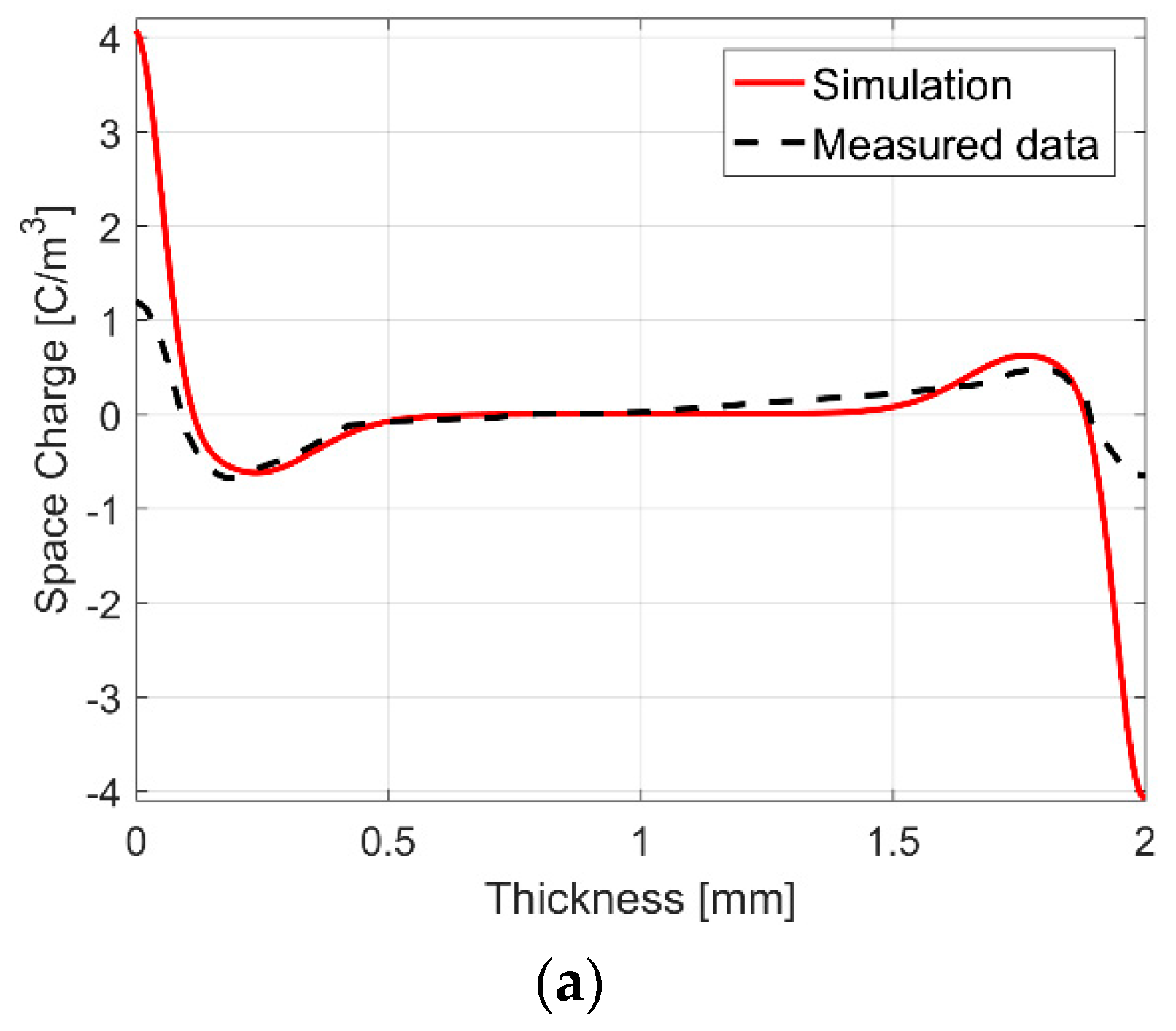
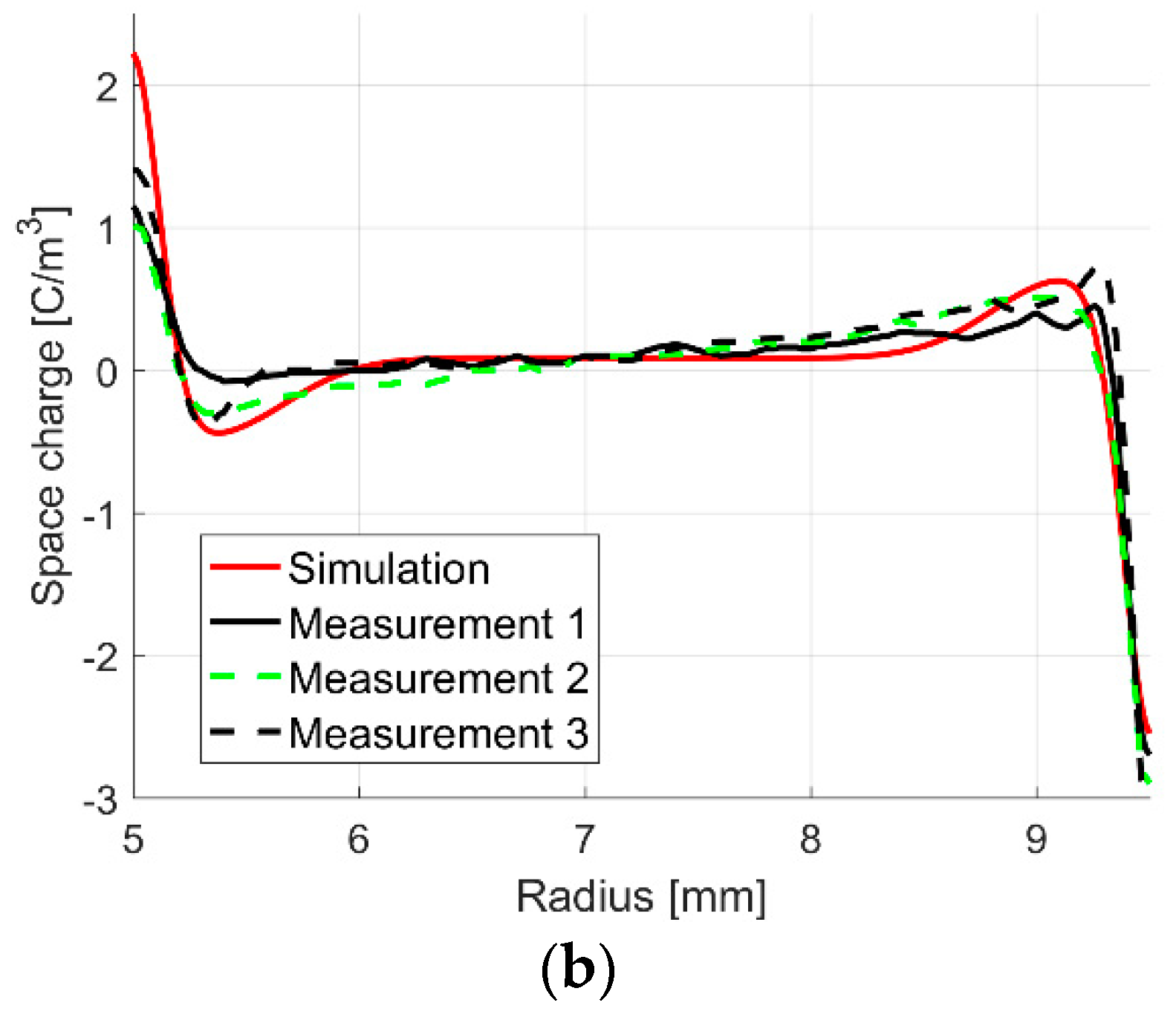
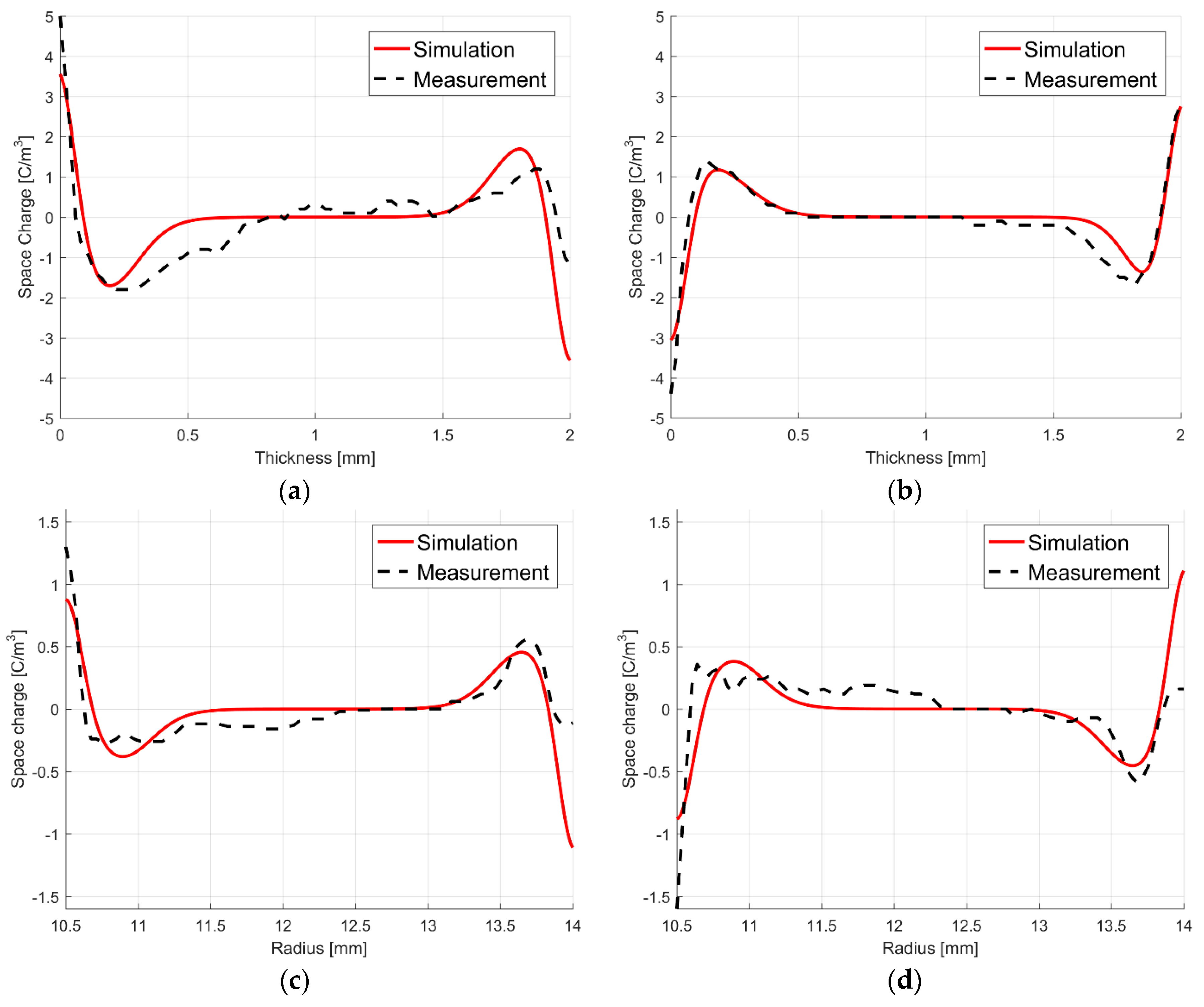
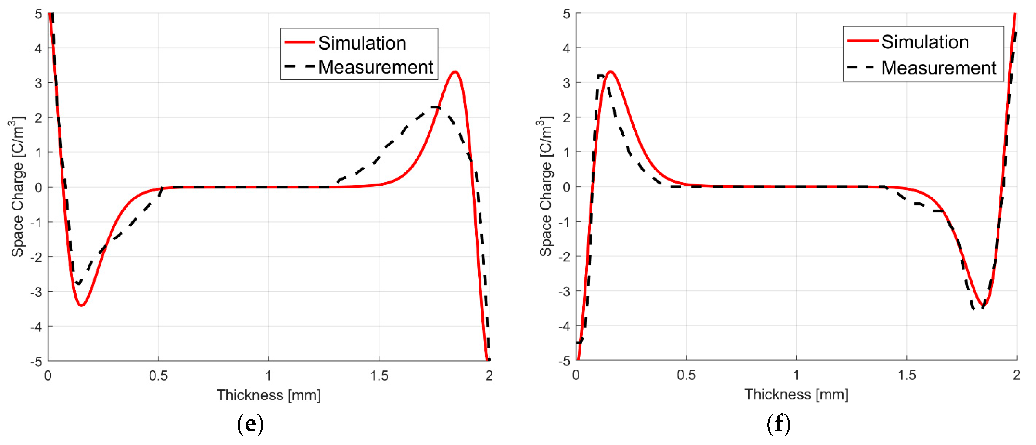
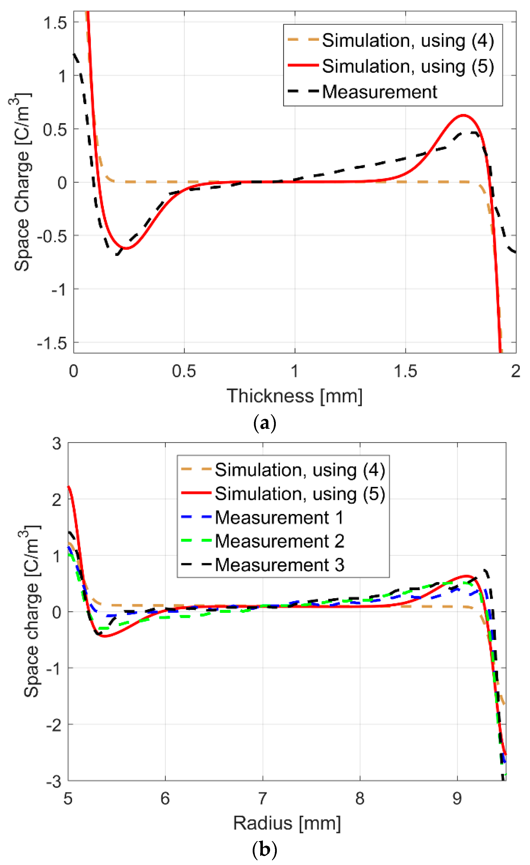
3.1. Measurements of XLPE Insulation

Space charge measurements in planplanar and cylindrical XLPE insulations are found in references [6,19,20]. Here, the measured hetero charge distribution, including the surface charges, is positioned in about one third of the insulation thickness in the vicinity of both electrodes, while the magnitude varies with a varying temperature and electric field strength. With a constant magnitude of the applied voltage and the opposite polarity, the charge density also changes the polarity, but shape and magnitude remain the same. This so called “mirror image effect” is reported and discussed e.g., in [23]. The inversion of the equilibrium space charge distribution is explained e.g., with a spatially inhomogeneous polarization of the dielectric and the injection of charges at the electrodes [24,25].

Steady state charge distributions in a planplanar insulation configuration (Figure 4a) and in a cylindrical geometry (Figure 4b) are simulated and depicted in Figure 4 [10,19,20].

In Figure 4b, three different XLPE cable measurements, labeled with numbers “1”–“3”, are seen. The cables differ for the semiconducting layer and the XLPE insulation type. The temperature in Figure 4a is constant (T = 27 °C), while in Figure 4b, a temperature gradient of 15 °C is used. The time independent temperature distribution is calculated by

$$T(r)=T_{\mathrm{i}}+\frac{T_{\mathrm{a}}-T_{\mathrm{i}}}{\ln \left(r_{\mathrm{a}}/r_{\mathrm{i}}\right)}\cdot \ln \left(r/r_{\mathrm{i}}\right),$$

(20)

where the inner temperature is T_i and the outer temperature is T_a.

In Figure 4a, the hetero charges and surface charges are simulated and measured, both processes including a Gaussian filtering, in a region of about 0.52 mm (0.26∙L) at each electrode. The used constants are χ = 0.052 mm = Δ/10 ≈ (0.26∙L)/10 and r_x = 0.25 mm = Δ/2 ≈ (0.26∙L)/2.

In Figure 4b, filtered hetero charges and surface charges are seen in a width of about 1 mm at each electrode, which is equal to 0.22 × (r_a − r_i). The used constants are χ = 0.12 mm = Δ/10 ≈ 0.22 × (r_a − r_i)/10 and r_x = 0.6 mm = Δ/2 ≈ 0.22 × (r_a − r_i)/2.

Comparing the simulation with “Measurement 1” indicate inaccurate results at the conductor and the sheath, where the simulation is overestimated. On the other hand, a comparison with “Measurement 2” and “Measurement 3” shows a sufficient accuracy of the simulated space charge distribution.

In Figure 4a, differences are observable especially at the anode and the cathode, which is a result of the filtering process. The computed surface charges (9) and (10) depend on the accumulated space charges and the local electric field. The local electric field depend on the space charges as well. If the simulated space charges differ in comparison to the measurement, the electric field and the surface charges also differ.

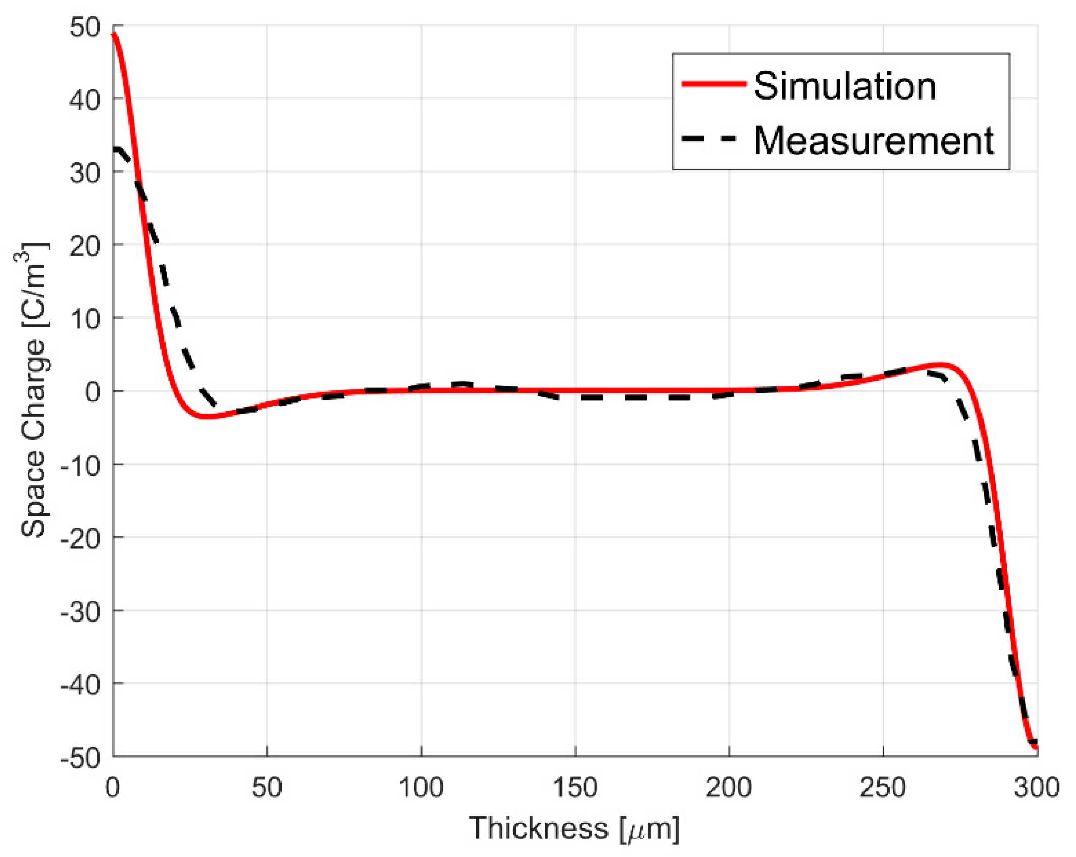
3.2. Measurements of LDPE Insulation

Measurements of a space charge distribution in a planplanar LDPE insulation are found e.g., in [6] and [21]. Simulation results and measurements of a 300 μm thick insulation are shown in Figure 5 [10,21]. The filtered hetero charges and surface charges accumulate in a region of approximately 80 μm at each electrode (0.267·L). The used constants are χ = 8 μm = Δ/10 ≈ 0.267·L/10 and r_x = 40 μm = Δ/2 ≈ 0.267·L/2.

In Figure 4 and Figure 5, the defined region of accumulated space charges is equal to the region of the conductivity gradient in Figure 2. Differences between the charge distribution in Figure 4 and Figure 5, compared to Figure 2b result from an assumed constant bulk conductivity in Figure 2. In Figure 4 and Figure 5 a temperature and electric field dependent bulk conductivity is utilized. Accumulated hetero charges change the electric field and the conductivity at both electrodes, resulting in a spread-out charge shape compared to Figure 2b. Furthermore, in Figure 4 and Figure 5, surface charges are considered and the simulation results are filtered, using a Gaussian filter [18].

Additional space charge simulations of XLPE and LDPE insulations are compared to measurements in [6]. The obtained results for the distance constant χ, the position r_x and the width of filtered surface and hetero charges Δ are seen in

Table 2. Distance constants χ and positions r_x for the simulation of space charge measurements in [6,19,20,21]. The absolute value of the applied voltage is |U| = 20 kV.

Ref.	χ	rx	Insulation Thickness	Width of Charge Region Δ
[20], Figure 4a	0.052 mm	0.25 mm	2 mm	0.26·L
[19], Figure 4b	0.12 mm	0.60 mm	4.5 mm	0.22 × (ra − ri)
[6], XLPE, planplanar, +U	0.052 mm	0.25 mm	2 mm	0.26·L
[6], XLPE, planplanar, −U	0.052 mm	0.25 mm	2 mm	0.26·L
[6], XLPE, cylindrical, +U	0.0875 mm	0.44 mm	3.5 mm	0.28 × (ra − ri)
[6], XLPE, cylindrical, −U	0.0875 mm	0.44 mm	3.5 mm	0.28 × (ra − ri)
[6], LDPE, planplanar, +U	0.052 mm	0.25 mm	2 mm	0.26·L
[6], LDPE, planplanar, −U	0.052 mm	0.25 mm	2 mm	0.26·L
[21], Figure 5	8 μm	40 μm	300 μm	0.267·L

. A comparison between the simulation results and the measurements are seen in Figure 6 [10]. Accumulated hetero charges (including surface charges) are seen in approximately one quarter of the insulation thickness, whereby the width Δ is approximately independent of the geometry or the insulation material (see Table 2). Due to the “mirror image effect” of the charge distribution, the values for χ and r_x are constant, while changing the polarity of the voltage. It is not clear, why the hetero charges accumulate in one quarter of the insulation thickness. The resolution of the PEA method is 1.6 μm for a one dimensional planplanar insulation with a thickness of 25–27,000 μm and 0.1–1 mm for a cable insulation with a thickness of 3.5–20 mm [26]. The resolution is accurate enough to separate between hetero charges and bulk space charges.

Comparing, the constants χ and r_x in (6) and (7) with the width Δ (region of filtered surface and hetero charges), the approximation χ = (0.25·L)/10 and r_x = (0.25·L)/2 for a planplanar insulation and χ = (0.25 × (r_a − r_i))/10 and r_x = (0.25 × (r_a − r_i))/2 for a cylindrical insulation is defined.

Using a temperature and electric field dependent electric conductivity, e.g., (4), only charges within the bulk are simulated, which are mainly a result of the temperature gradient. Thus, comparing the measurements and the simulations, high differences are observable in the vicinity of the electrodes. For example, Figure 7 shows a space charge measurement and the simulating results using a commonly utilized conductivity Equation (4) and using (5). The applied constants are equal to the constants for Figure 4a,b and are seen in Table 1. Without a temperature gradient and electric field gradient, (4) is constant within the insulation and the simulated space charge density ρ = 0 C/m³ (see (8)). The surface charges (17) and (18) are reduced to ${\delta }_{+}={\epsilon }_0{\epsilon }_{\mathrm{r}}(r_{\mathrm{i}})|\overrightarrow{E}(r_{\mathrm{i}})|$ and ${\delta }_{-}={\epsilon }_0{\epsilon }_{\mathrm{r}}(r_{\mathrm{a}})|\overrightarrow{E}(r_{\mathrm{a}})|$ (see Figure 7a). A temperature gradient along the insulation results in accumulated bulk space charges, which are lower in the vicinity of the electrodes, compared to the measurements (see Figure 7b).

The conductivity of polymeric insulation materials differs with the sample preparation, which effects the constants $|J_0|$, E_a, and γ in (4). The resulting space charge distribution depends on many factors e.g., the conductivity, the local electric field, or the electrode material. As a result, it is very difficult to simulate the charge distribution of different references, even if it is the same material, like XLPE [27,28]. Differences between the measurements and the simulations in Figure 4, Figure 5 and Figure 6 are small and the developed model yield results with good agreement to the measurements. The developed conductivity equation shows less differences to measurements compared to a commonly used conductivity equation and thus, the applicability of the formulation.

4. Conclusions

An empirical conductivity model equation was developed for XLPE and LDPE insulation materials. As various space charge measurements in literature showed accumulated hetero charges in the vicinity of both electrodes, to simulate these charges, a commonly established, but insufficient accurate nonlinear field and temperature dependent conductivity model was used and improved by two sigmoid functions to create a conductivity gradient at both electrodes. The model was validated with its steady state space charge distribution and resulted in realistic accumulation of hetero charges typically positioned in about one quarter of the insulation thickness at each electrode. A comparison of simulation and measurement results validated the presented model, showing a good agreement and an improvement in comparison to those of previously established conductivity models.

References

1. Hanley, T.L.; Burford, R.P.; Fleming, R.J.; Barber, K.W. A general review of polymeric insulation for use in HVDC cables. IEEE Electr. Insul. Mag. 2003, 19, 14–24. [Google Scholar] [CrossRef]
2. Dissado, L.A. The origin and nature of ‘charge packets’: A short review. In Proceedings of the International Conference on Solid Dielectrics, Potsdam, Germany, 4–9 July 2010; pp. 1–6. [Google Scholar] [CrossRef]
3. Fleming, R.J. Space Charge in Polymers, Particularly Polyethylene. Braz. J. Phys. 1999, 29, 280–294. [Google Scholar] [CrossRef]
4. Küchler, A. High Voltage Engineering–Fundamentals, Technology, Applications, 5th ed.; Springer: Berlin/Heidelberg, Germany, 2018; pp. 583–590, 503–507. [Google Scholar] [CrossRef]
5. Fabiani, D.; Montanari, G.C.; Dissado, L.A.; Laurent, C.; Teyssedre, G. Fast and Slow Charge Packets in Polymeric Materials under DC Stress. IEEE Trans. Dielectr. Electr. Insul. 2009, 16, 241–250. [Google Scholar] [CrossRef]
6. Wang, X.; Yoshimura, N.; Murata, K.; Tanaka, Y.; Takada, T. Space-charge characteristics in polyethylene. J. Phys. D Appl. Phys. 1998, 84, 1546–1550. [Google Scholar] [CrossRef]
7. Takeda, T.; Hozumi, N.; Suzuki, H.; Okamoto, T. Factors of Hetero Space Charge Generation in XLPE under dc Electric Field of 20 kV/mm. Electr. Eng. Jpn. 1999, 129, 13–21. [Google Scholar] [CrossRef]
8. Jörgens, C.; Clemens, M. Modeling the Field in Polymeric Insulation Including Nonlinear Effects due to Temperature and Space Charge Distributions. In Proceedings of the Conference on Electrical Insulation and Dielectric Phenomena (CEIDP), Fort Worth, TX, USA, 22–25 October 2017; pp. 10–13. [Google Scholar] [CrossRef]
9. Hjerrild, J.; Holboll, J.; Henriksen, M.; Boggs, S. Effect of Semicon-Dielectric Interface on Conductivity and Electric Field Distribution. IEEE Trans. Electr. Insul. 2002, 9, 596–603. [Google Scholar] [CrossRef]
10. Jörgens, C.; Clemens, M. Empirical Conductivity Equation for the Simulation of Space Charges in Polymeric HVDC Cable Insulations. In Proceedings of the 2018 IEEE International Conference on High Voltage Engineering and Application (ICHVE), Athene, Greece, 10–13 September 2018. [Google Scholar] [CrossRef]
11. LeRoy, S.; Segur, P.; Teyssedre, G.; Laurent, C. Description of bipolar charge transport in polyethylene using a fluid model with constant mobility: Model predictions. J. Phys. D Appl. Phys. 2003, 37, 298–305. [Google Scholar]
12. Wintle, H.J. Charge Motion and Trapping in Insulators–Surface and Bulk Effects. IEEE Trans. Electr. Insul. 1999, 6, 1–10. [Google Scholar] [CrossRef]
13. Bodega, R. Space Charge Accumulation in Polymeric High Voltage DC Cable Systems. Ph.D. Thesis, Delft University of Technology, Delft, The Netherlands, 2006; pp. 78–88. [Google Scholar]
14. Kumara, J.R.S.S.; Serdyuk, Y.V.; Gubanski, S.M. Surface Potential Decay on LDPE and LDPE/Al2O3 Nano-Composites: Measurements and Modeling. IEEE Trans. Dielectr. Electr. Insul. 2016, 23, 3466–3475. [Google Scholar] [CrossRef]
15. Boudou, L.; Guastavino, J. Influence of temperature on low-density polyethylene films through conduction measurement. J. Phys. D Appl. Phys. 2002, 35, 1555–1561. [Google Scholar] [CrossRef]
16. Bambery, K.R.; Fleming, R.J.; Holboll, J.T. Space charge profiles in low density polyethylene samples containing a permittivity/conductivity gradient. J. Phys. D Appl. Phys. 2001, 34, 3071–3077. [Google Scholar] [CrossRef]
17. Fleming, R.J.; Henriksen, M.; Holboll, J.T. The Influence of Electrodes and Conditioning on Space Charge Accumulation in XLPE. IEEE Trans. Electr. Insul. 2000, 7, 561–571. [Google Scholar] [CrossRef]
18. Lv, Z.; Cao, J.; Wang, X.; Wang, H.; Wu, K.; Dissado, L.A. Mechanism of Space Charge Formation in Cross Linked Polyethylene (XLPE) under Temperature Gradient. IEEE Trans. Dielectr. Electr. Insul. 2015, 22, 3186–3196. [Google Scholar] [CrossRef]
19. Bodega, R.; Morshuis, P.H.F.; Straathof, E.J.D.; Nilsson, U.H.; Perego, G. Characterization of XLPE MV-size DC Cables by Means of Space Charge Measurements. In Proceedings of the Conference on Electrical Insulation and Dielectric Phenomena (CEIDP), Kansas City, MO, USA, 15–18 October 2006; pp. 11–14. [Google Scholar] [CrossRef]
20. Mizutani, T. Space Charge Measurement Techniques and Space Charge in Polyethylene. IEEE Trans. Dielectr. Electr. Insul. 1994, 1, 923–933. [Google Scholar] [CrossRef]
21. Wu, J.; Lan, L.; Li, Z.; Yin, Y. Simulation of Space Charge Behavior in LDPE with a Modified of Bipolar Charge Transport Model. In Proceedings of the International Symposium on Electrical Insulating Materials, Niigata, Japan, 1–5 June 2014; pp. 65–68. [Google Scholar] [CrossRef]
22. Jörgens, C.; Clemens, M. Conductivity-based model for the simulation of homocharges and heterocharges in XLPE high-voltage direct current cable insulation. IET-SMT 2019. [Google Scholar] [CrossRef]
23. Fu, M.; Dissado, L.A.; Chen, G.; Fothergill, J.C. Space Charge Formation and its Modified Electric Field under Applied Voltage Reversal and Temperature Gradient in XLPE Cable. IEEE Trans. Electr. Insul. 2008, 15, 851–860. [Google Scholar] [CrossRef]
24. Bambery, K.R.; Fleming, R.J. Space Charge Accumulation in Two Power Cables Grades of XLPE. IEEE Trans. Dielectr. Electr. Insul. 1998, 5, 103–109. [Google Scholar] [CrossRef]
25. Lim, F.N.; Fleming, R.J.; Naybour, R.D. Space Charge Accumulation in Power Cable XLPE Insulation. IEEE Trans. Dielectr. Electr. Insul. 1999, 6, 273–281. [Google Scholar] [CrossRef]
26. Imburgia, A.; Miceli, R.; Sanseverino, E.R.; Romano, P.; Viola, F. Review of Space Charge Measurement Systems: Acoustic, Thermal and Optical Methods. IEEE Trans. Dielectr. Electr. Insul. 2015, 23, 3126–3142. [Google Scholar] [CrossRef]
27. Karlsson, M.; Xu, X.; Gaska, K.; Hillborg, H.; Gubanski, S.M.; Gedde, U.W. DC Conductivity Measurements of LDPE: Influence of Specimen Preparation Method and Polymer Morphology. In Proceedings of the 25th Nordic Insulation Symposium, Västerås, Sweden, 19–21 June 2017. [Google Scholar] [CrossRef]
28. Xu, X.; Gaska, K.; Karlsson, M.; Hillborg, H.; Gedde, U.W. Precision electric characterization of LDPE specimens made by different manufacturing processes. In Proceedings of the 2018 IEEE International Conference on High Voltage Engineering and Application (ICHVE), Athene, Greece, 10–13 September 2018. [Google Scholar] [CrossRef]
Figure 1. (a) geometry of a planplanar insulation; (b) geometry of a cylindrical insulation [10].
Energies 12 03018 g001
Figure 2. Influence of distance constant χ on conductivity gradient and resulting space charge distribution ρ. (a) normalized conductivity σ/σB; (b) normalized stationary space charge distribution [10].
Energies 12 03018 g002
Figure 3. (a) Gradient region Δ, where the conductivity gradient is present. The position r = rx = Δ/2 has the highest gradient; (b) to determine χ by Δ, a straight line f(x) = a(xrx) + 0.5 = (1/Δ)(xrx) + 0.5 is used, where the best approximation is shown by Δ = 10χ [10].
Energies 12 03018 g003
Figure 4. (a) Measured and simulated charge distribution in a planplanar cross-linked polyethylene (XLPE) insulation [20]; (b) Measured and simulated charge distribution in a cylindrical XLPE insulation. Three different XLPE cable measurements, labeled with numbers “1”–“3”, are seen [10,19].
Energies 12 03018 g004aEnergies 12 03018 g004b
Figure 5. Measured and simulated charge distribution in a planplanar low-density polyethylene (LDPE) insulation [10,21].
Energies 12 03018 g005
Figure 6. Measured and simulated charge distribution in a XLPE and LDPE insulation [6]. (a) XLPE, planplanar, +U; (b) XLPE, planplanar, −U; (c) XLPE, cylindrical, +U; (d) XLPE, cylindrical, −U; (e) LDPE, planplanar, +U; (f) LDPE, planplanar, −U. The absolute value of the applied voltage is |U| = 20 kV.
Energies 12 03018 g006aEnergies 12 03018 g006b
Figure 7. (a) Measured and simulated charge distribution, using a common conductivity equation in literature (4) and the developed conductivity equation (5) in a planplanar XLPE insulation [20]; (b) Measured and simulated charge distribution, using (4) and (5) in a cylindrical XLPE insulation [19].
Energies 12 03018 g007