Article

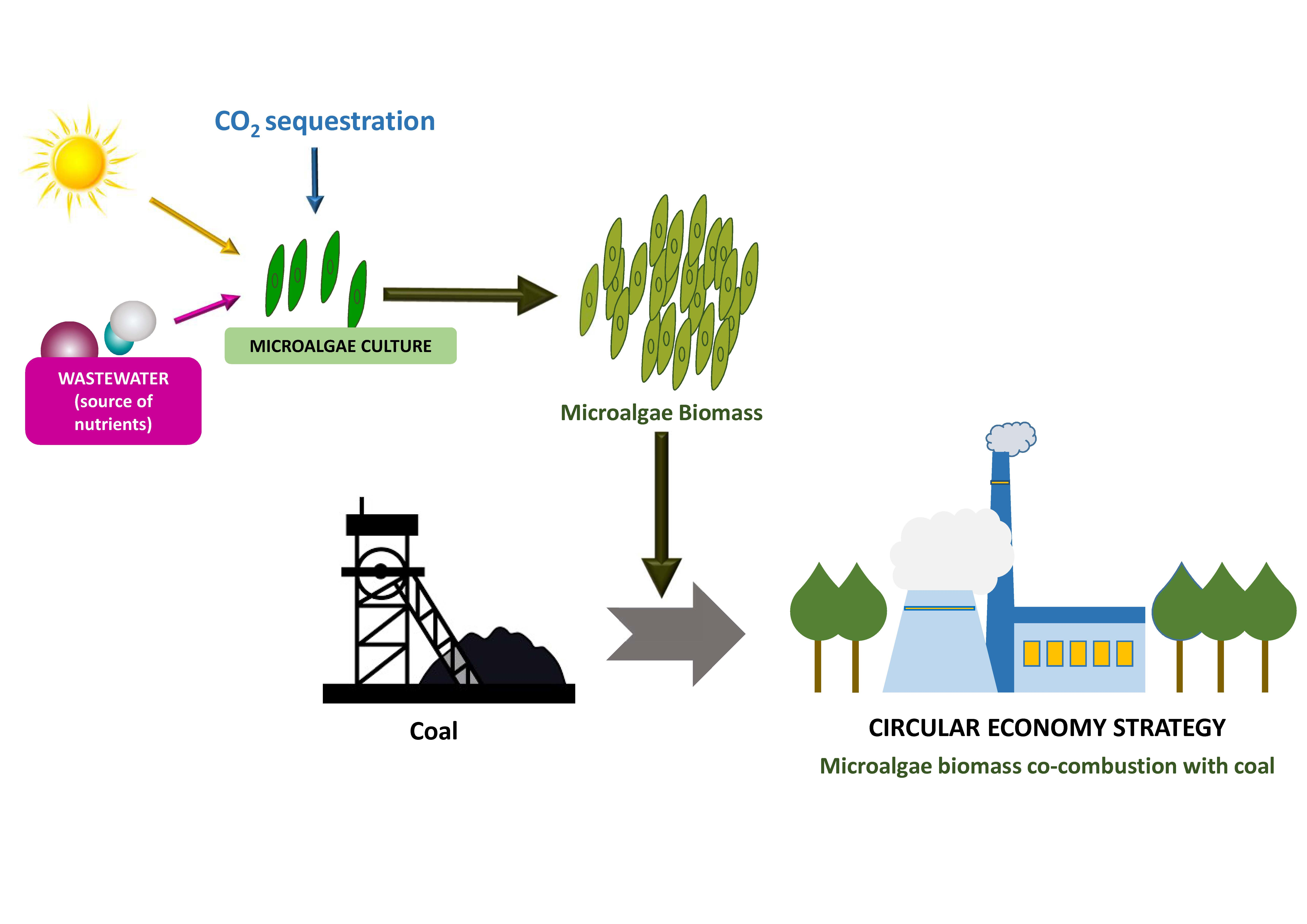
Comparative Thermogravimetric Assessment on the Combustion of Coal, Microalgae Biomass and Their Blend

1
Department of Environment and Planning, University of Aveiro, Campus Universitário de Santiago, 3810-193 Aveiro, Portugal
2
Department of Applied Chemistry and Physics, Institute of Environment, Natural Resources and Biodiversity (IMARENABIO), Universidad de León, 24071 León, Spain
3
Centre for Environmental and Marine Studies (CESAM), University of Aveiro, Campus Universitário de Santiago, 3810-193 Aveiro, Portugal
*
Author to whom correspondence should be addressed.
Energies 2019, 12(15), 2962; https://doi.org/10.3390/en12152962
Submission received: 5 July 2019 / Revised: 25 July 2019 / Accepted: 29 July 2019 / Published: 1 August 2019
(This article belongs to the Special Issue Advances in Combustion of Gases, Liquid Fuels, Coal and Biomass)

Abstract

:
In this work, thermogravimetric analysis (TGA), differential thermogravimetry (DTG), and differential scanning calorimetric (DSC) were used to assess the combustion of microalgae biomass, a bituminous coal, and their blend. Furthermore, different correlations were tested for estimating the high heating value of microalgae biomass and coal, with both materials possessing similar values. TGA evidenced differences between the combustion of the studied fuels, but no relevant interaction occurred during their co-combustion, as shown by the DTG and DSC curves. These curves also indicated that the combustion of the blend mostly resembled that of coal in terms of weight loss and heat release. Moreover, non-isothermal kinetic analysis revealed that the apparent activation energies corresponding to the combustion of the blend and coal were quite close. Overall, the obtained results indicated that co-combustion with coal might be a feasible waste to energy management option for the valorization of microalgae biomass resulting from wastewater treatment.

Graphical Abstract

1. Introduction

The rapid growing of population continuously increases the global demand for energy. This demand is actually mainly satisfied by the consumption of oil followed by coal, which remain the world’s leading fuels, respectively accounting for 33% and 30% of global energy consumption [1]. Such an extensive use is leading to the depletion and ever-rising prices of these fossil non-renewable fuels [2]. On the other hand, greenhouse gases emission from burning of fossil fuels, mainly CO2, is the main cause of global warming [3]. These facts have motivated increasing research efforts regarding alternative and/or non-conventional energy resources. Among them, biomass, which may be categorized into first, second, and third generation according to its origin, has been recognized as a promising option, since it is sustainable, renewable, and less polluting [2,3,4].
Microalgae biomass may be considered to be a third generation biofuel, which holds several advantages, such as microalgae rapid growth rate, high oil content, high yield per area, no competition with crops for arable land or freshwater [5,6]. Furthermore, microalgae are considered as promising candidates for CO2 bio-sequestration [7]. However, the implementation of CO2 sequestration by microalgae is mostly limited by techno-economic constrains [8]. Microalgae may be cultivated in wastewater, allowing for simultaneous CO2 mitigation and wastewater treatment [7]. In order to increase economic feasibility [7]. In this way, wastewater is used as source of nutrients and water, which allows for reducing the costs of microalgae culturing [5,9,10]. On the other hand, microalgae are efficient microorganisms for wastewater treatment, since they are able to remove not only nutrients, but also heavy metals [11] and emerging contaminants [12,13]. Still, during microalgae cultivation, residual biomass is generated and use should be given to this biomass within the actual circular economy context [14]. Therefore, the utilization of microalgae biomass as a third generation biofuel might be an option for closing the loop and increasing the sustainability of microalgae culture [8]. In this sense, integrating microalgae culture-wastewater treatment-biofuel production allows for carbon dioxide mitigation and wastewater treatment, while providing biofuel feedstock in a much cleaner manner [7,15].
Biomass thermochemical conversion is considered to be one of the most effective and promising routes aimed at the use of biomass for energy purposes. Thermochemical processes typically include [16]: pyrolysis, gasification and combustion, which is the most commonly used pathway to extract energy from biomass [17]. Algal biomass has lower decomposition temperatures during thermochemical conversion when compared to lignocellulosic biomass, which is due to differences in their major components and results in higher reactivity and lower operational costs [18]. In any case, a good understanding of microalgae behaviour during thermochemical conversion is essential in efficient processing.
The utilization of thermogravimetric analysis (TGA) for the characterization of thermal decomposition during the combustion of coal is well established, being more recent its use for biomassic fuels [19] and their co-processing with coal [20,21,22]. Such utilization is advantageous, since TGA offers a rapid evaluation of the thermal decomposition of any fuel, the initial and final temperatures of combustion, and other important features, such as maximum reactivity temperature or interaction between fuels during co-processing [19,23].
Comparatively with lignocellulosic biomass, only very recent and few works are concerned about the thermal analysis of microalgae combustion [18] and studies on the co-combustion of microalgae biomass with fossil fuels, such as coal, are even scarcer. However, co-combustion with fossil fuels is an interesting option that may help to reduce the consumption of non-renewable resources for power generation, while allowing for the utilization of existing infrastructures. Thus, in this manuscript, simultaneous TGA and differential scanning calorimetry (DSC) were used to assess the combustion behaviour of microalgae biomass and its blend with coal. The main aims were to evaluate the effect that blending with microalgae biomass has on the combustion of coal and its kinetics and to find out whether interactions between both fuels occur during their co-combustion.

2. Materials and Methods

2.1. Microalgae Culturing

For this study, Chlorella sorokiniana CCAP 211/8 K (UTEX Culture Collection) was cultured in axenic conditions. This strain was chosen because Chlorella sp. is amongst the most commonly used for wastewater treatment, possesses high growth rates, high light to biomass conversion, ability to grow under phototrophic, photomixotrophic and heterotrophic conditions, high protein amount, essential amino acids, and fatty acids [24,25]. On the other hand, as compared with C. vulgaris, the thermal decomposition of C. sorokiniana has been less studied in the literature.
The inoculum of C. sorikiniana was cultivated in 250 mL Erlenmeyer flasks in the standard culture medium Mann and Myers [26], which is composed of (per litre of distilled water): 1.2 g MgSO4·7H2O, 1.0 g NaNO3, 0.3 CaCl2, 0.1 g K2HPO4, 3.0 × 10⁻² g Na2EDTA, 6.0 × 10⁻³ g H3BO3, 2.0 × 10⁻³ g FeSO4·7H2O, 1.4 × 10⁻³ g MnCl2, 3.3 × 10⁻⁴ g ZnSO4·7H2O, 7.0 × 10⁻⁶ g Co(NO3)2·6H2O, 2.0 × 10⁻⁶ g CuSO4·5H2O. This inoculum was grown under constant temperature (25 ± 1 °C), irradiance (175 µE/m2·s), photoperiod (12:12), and shaking (250 rpm) until reaching a biomass concentration of 0.1 g/L. Afterwards, the culture was grown in a 10 L-PBR after acclimatization to synthetic wastewater in 1 L-bubbling column photobioreactors (PBRs) and growing up to 0.1 g/L of biomass concentration. Each litre of synthetic wastewater was prepared by dissolving in distilled water: peptone, 160 mg; meat extract, 110 mg; urea, 30 mg; anhydrous dipotassium hydrogen phosphate (K2HPO4), 28 mg; sodium chloride (NaCl), 7 mg; calcium chloride dehydrate (CaCl2·2H2O), 4 mg; and, magnesium sulphate heptahydrate (Mg2SO4·7H2O), 2 mg. This synthetic wastewater [27] gives a mean DOC concentration of about 100 mg/L. The culture conditions and medium used for the inoculum growth were maintained for microalgae growth in the PBRs, except for the irradiance, which was 650 µE/m2·s, as supplied by eight fluorescent lamps (58 W, 2150 lumen, Philips, France). Furthermore, the PBRs were aerated with filtered air (0.22 µm sterile air-venting filter, MillexFG50-Millipore), at a rate of 0.3 v/v/min., enriched with CO2 at 7% v/v, which was injected on demand to keep a constant pH (pH = 7.5 ± 0.5), as controlled by a pH sensor. At the end of the culture, the 10 L-PBR was dismantled, and microalgae biomass was harvested by 5 min centrifugation of the cellular suspension at 6461 g in a SIGMA 2-16P centrifuge. Microalgae biomass (MB) was then washed twice with distilled water, oven dried during 24 h at 378 K, homogenized, and stored until use at 277 K.

2.2. Materials and Characterization

MB and a bituminous coal (BC) coming from the north coalfield of León (Spain) and commonly exploited in thermal power stations were used in this work. Before thermal analysis, MB and BC were grinded and sieved to have a 0.105 mm < particle diameter < 0.210 mm, which is within the size range that is commonly used in circulating fluidized boilers, allows for minimization of differences in heat of combustion values, and is large enough to ensure homogeneous ignition. Subsequently, proximate analyses of MB and BC were carried out following the procedures from ASTM D3172 to D3175 [28,29,30,31]. Elemental analysis was performed in a LECO CHNS-932, according to standard procedures, namely ASTM D5373 [32] and ASTM D4239 [33].
The high heating value (HHV) of MB and BC at a constant volume was determined by means of an isoperibol oxygen bomb calorimeter LECO AC-600 and following the procedure UNE-EN 14918:2011 [34]. Additionally, and for comparison purposes, HHV was estimated by the correlations that are listed in Table 1, together with the corresponding assumptions.

2.3. Thermal Analyses

A Setaram equipment, model SETSYS Evolution was used in this work. Non-isothermal combustion runs were carried out after calibration for baseline, weight, temperature, and heat flow. Throughout these runs, Thermogravimetry (TG) and Differential Scanning Calorimetry (DSC) signals were simultaneously registered during the temperature-programmed combustion of MB, BC, and their blend (MB-BC). In the blend, a 10% wt. of MB was used, since it has been shown that such a percentage is adequate for the practical implementation of co-combustion of coal with biomass in existing infrastructures, namely in thermal power plants [20]. Derivative TG (DTG) curves were also determined as the first derivation of TG results with respect to time. The runs were carried out up to 1200 K at four different heating rates (β = dT/dt): 0.1, 0.2, 0.4, and 0.5 K/s, in order to determine the corresponding TG-DSC curves. For each sample and β, three repetitive runs were carried out using 15 ± 1 mg of MB, BC, or MB-BC, after having verified that this mass ensured representativeness and avoided heat and/or mass transfer limitations. All the runs were done under a continuous air flow (100 cm3/min at 1 atm of gauge pressure).
The theoretical DTG curves (DTG(T)) and DSC curves (DSC(T)) were calculated for the blend MB-BC using Equations (1) and (2), respectively, as a weighted average of its composition in order to check interaction between MB and BC during their co-combustion:
DTG(T) = 0.1 × DTGMB + 0.9 × DTGBC
where DTGMB and DTGBC are the weight loss rate of MB and BC throughout their respective temperature-programmed combustions.
DSC(T) = 0.1 × DSCMB + 0.9 × DSCBC
where DSCMB and DSCBC are the differential scanning calorimetry results that correspond to the temperature-programmed combustion of MB and BC, respectively.

2.4. Non-Isothermal Kinetic Analysis

The rate of heterogeneous solid state reactions is generally described by the following equation:
d α d t = k ( T ) f ( α )
where α is the extent of reaction or fractional conversion, t is time, T is temperature, k(T) is the temperature-dependent constant, and f(α) is a function that describes the dependence of the reaction rate on α.
Usually, the decomposition from a solid state is mathematically described in terms of the kinetic triplet (apparent activation energy (E), pre-exponential factor (A), and an expression of the kinetics in terms of f(α)), which may be correlated to the obtained results by this rate expression:
d α d t = A e E / R T f ( α )
The previous rate expression (Equation (4)) may be transformed into a non-isothermal one, which defines the reaction rate in function of T at a constant β:
d α d T = A β A e E / R T f ( α )
When Equation (5) is integrated up to α, results in:
0 α d α f ( α ) = g ( α ) = A β T 0 T e E / R T d T
where g(α) is the integral reaction model.
Several methods may be used in order to obtain a description of the combustion process in terms of E [48]. These methods can be classified depending on the experimental conditions and on the mathematical analysis that was carried out. As for the experimentation, the results may be obtained either under isothermal or non-isothermal conditions. Regarding mathematical analysis, either the model-fitting or the iso-conversional (model-free) approaches may be followed.
For non-isothermal kinetic analysis, different iso-conversional models that involve carrying out temperature-programmed runs at different β [48] have been developed to determine E. During the last decade, these methods have been frequently used to study the thermal decomposition kinetics of very different types of biofuels [20,21], including microalgae biomass [49].
In this sense, E may be estimated by applying the iso-conversional model developed by Flynn, Wall, and Ozawa [50,51], which is an integral method that uses the Doyle’s approximation [52]:
ln ( β ) = l n [ A E R   g ( α ) ] 5.331 1.052 E R T
The utilization of the Flynn-Wall-Ozawa (FWO) method [50,51] requires the determination of the T corresponding to fixed values of α from runs carried out at different β. E is estimated by plotting ln(β) vs. 1/T for each α, which gives straight lines with slope—E/R.
E may be also determined on the basis of the Kissinger-Akahira-Sunose (KAS) kinetic model [53,54], as it is next described.
In Equation (5) E/2RT » 1, therefore, the integral can be approximated by:
T 0 T e E / R T d T R E T 2 e E / R T
Substituting the temperature integral and taking the logarithm:
ln β T 2 = ln [ R A E g ( α ) ] E R 1 T
For the application of the KAS model [53,54], it is necessary to carry out runs at different β, the respective conversion curves being evaluated from the measured TG curves. For each α, ln(β/T2) plotted versus 1/T gives a straight line with slope −E/R.

3. Results and Discussion

3.1. Materials Characterization

The results from the proximate and elemental analyses of MB and BC are depicted in Table 2, together with the measured HHV for each material.
As may be seen in Table 2, the proximate and elemental analyses of MB and BC evidence that these fuels have very distinct properties due to their different origin and nature. Within the proximate analysis, moisture percentages for both materials are usual equilibrium values for storeroom conditions. With respect to the ash yield, it is quite smaller for MB (6.2%) than for BC (31.1%), which is a positive fact for the biofuel utilization of MB, since relatively high ash contents are undesirable in many combustion facilities. However, the amount of volatiles in MB (78.2%) is much larger than in BC (8.2%). The higher volatile matter content of biomass, as compared with coal, is known to improve the combustion of the latter, which results in a better burn out and lower unburned carbon in the ashes [21]. Still, adaptations of the combustor may be necessary for the co-processing of fuels with very different volatiles content. On the other hand, due to the higher volatile content of MB, it possesses a lower fixed-carbon (15.6%) than BC (60.7%), which is expected to be corroborated in their separate combustion DTG profiles.
Regarding the elemental analysis, BC has a higher C content (62.7%) than MB (52.0%). Contrarily, BC has much lower O content (1.7%) than MB (29.8%). Additionally, the H and N contents of BC (2.5 and 1.3%, respectively) are lower than those of MB (6.8 and 10.7%, respectively). Nonetheless, it has been demonstrated that NO emissions are not strongly dependent on the fuel nitrogen content [55]. Meanwhile, both BC and MB have a similar S content (0.7 and 0.6%, respectively), so their combustion may involve similar SOx emissions.
The results from proximate and elemental analyses of MB are very similar to those that were determined for C. vulgaris biomass by Gao et al. [56]. However, slightly different results have been obtained by other authors for C. vulgaris biomass [57], being especially relevant the comparatively higher volatiles content and lower percentage of ashes of MB. The differences are probably related to the specific strain and the way or stage of culturing. In fact, nitrogen supplementation [58] and the age of the culture [59] have already been shown to affect thermal properties of C. sorokiniana. Regarding BC, the results are comparable to previously published data for coal with the same rank and origin [23].
Finally, as regards the HHV, both MB and BC have very similar values (22.9 and 24.3 MJ/kg, respectively), which means that the combustion of their blend is not going to have remarkable energetic effects as compared with the combustion of BC. The HHV determined in this work for MB is within the range of values referred in the review by Chen et al. [4], namely 14 to 24 MJ/kg, while the HHV of BC is close to published data for coal with the same rank and origin [23].
As for the estimation of HHV, Figure 1 shows the values that were obtained by the correlations depicted in Table 1 for each MB and BC, together with the measured value and a deviation limit of ±10%. Some of the correlations satisfactorily estimate the HHV of MB and BC, mainly those that are based on elemental or on both elemental and proximate analyses. However, correlations that are only based on proximate analysis (No. 7–11 in Table 1) mostly underestimate the HHV, except for correlation No. 10 [43], which overestimates the HHV of MB, and correlations No. 8 [42] and 10 [43], which only give an acceptable HHV estimation for BC. Correlation No. 1, which is the well-known Dulong correlation [35] and is just based on the C, H, and O contents, correlation No. 4 [38], which also depends on the C, H and O contents, and correlation No. 14 [46], which stands on the elemental analysis and the ash content, are those that more closely estimate the HHV for both MB and BC. These correlations may be very useful for the quick estimation of the calorific potential of microalgae and coal when planning their co-processing.
To the best of our knowledge, there are no published studies using correlations for the estimation of HHV in the specific case of microalgae biomass. Therefore, the applicability of the here considered correlations (Table 1) was tested in this work for available data in the literature on the calorific value of microalgae biomass from different strains. In the case of those microalgae biomasses for which just the elemental analysis is available, the estimated HHV values are depicted in Table 3. For biomasses whose elemental and proximate analyses are available, the estimations of HHV are displayed in Table 4.
As may be observed in Table 4, estimations that are just based on proximate analyses (correlations No. 7 to 11 in Table 1) are mostly inadequate, while those that are just based on the elemental analysis (Table 3) or elemental analysis together with proximate analysis (Table 4) give estimations that are more satisfactory. On the whole, and coincidently with the case of microalgae biomass that was obtained in this work, correlations No. 1, 4, and, especially, No. 14 were the most accurate for estimating the HHV of microalgae biomasses in the literature.

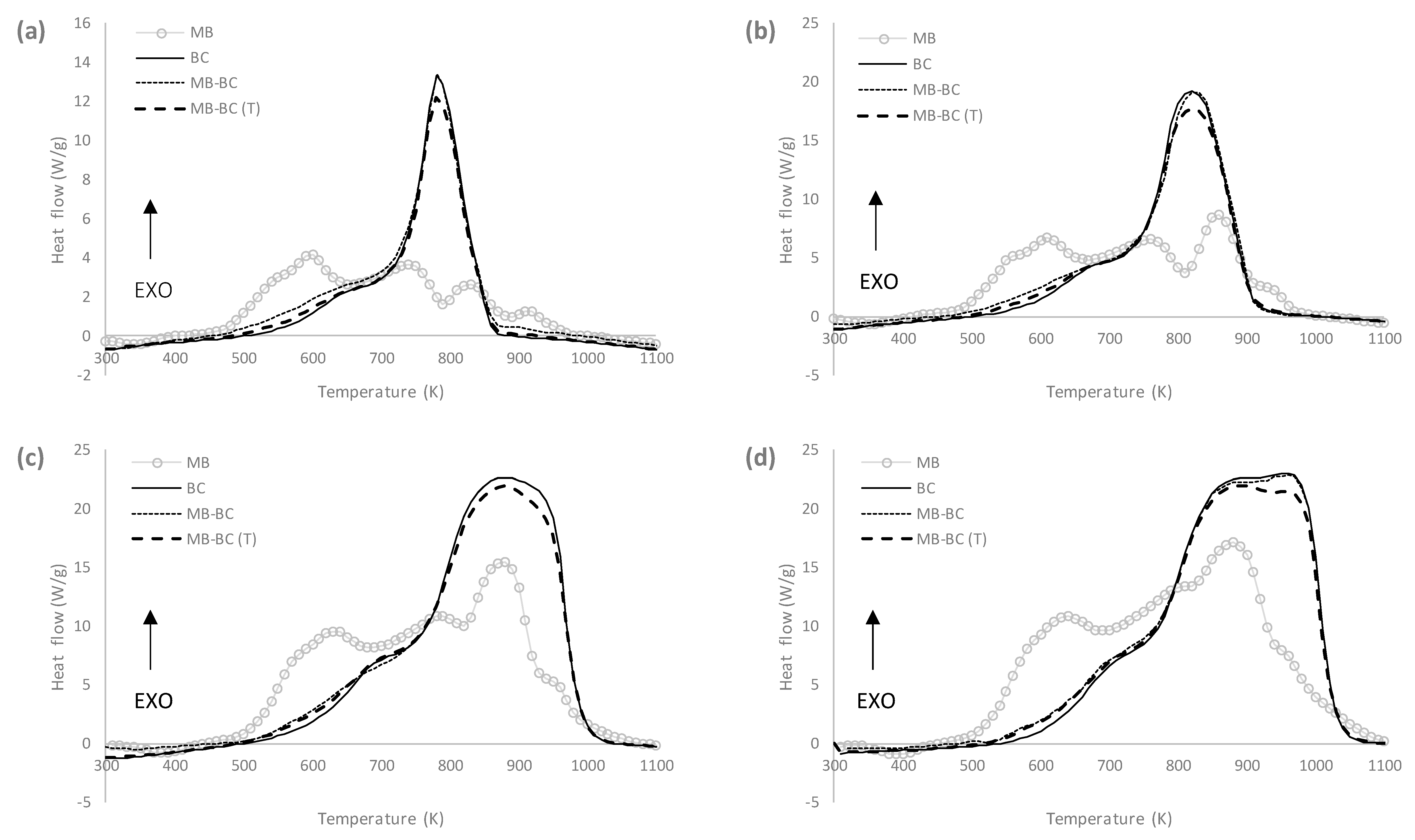
3.2. Thermal Analysis

The TG curves that were obtained from the temperature programmed combustion of MB, BC, and their blend MB-BC at different β (0.1, 0.2, 0.4, and 0.5 K/s) are depicted in Figure S1. The resultant DTG curves are shown in Figure 2 together with the weighted calculated curves (Equation (1)) corresponding to the combustion of MB-BC. As for a typical combustion profile, mass loss occurs along with increasing temperature under oxidizing atmosphere until the volatiles and fuel content of the sample is exhausted, and then the mass of ashes remains stable. In the case of BC, the loss of volatiles and char gasification occur in a single step due to the large contribution of fixed carbon (see Table 2) to the mass loss during combustion. On the other hand, a slight weight gain that is related to oxygen chemisorption may be observed during the combustion of BC but is not present in the DTG curves corresponding to MB. Differently from BC, the DTG curve that corresponds to MB shows that mass loss occurs in two main stages, which has already observed by other authors for the combustion of microalgae [16,56,57]. The first stage, which is the most remarkable, is attributed to the devolatilization of MB and volatiles combustion and extends until 670 K. It is to highlight that this first stage occurs in a temperature range for which no mass loss is observed for BC. This is due to the higher volatiles/fixed-carbon ratio of MB (5.01), as compared to that of BC (0.13), which involves microalgae combustion predominantly occurring in gas-phase due to the combustion of volatiles. Above 670 K and ending at around 1000 K, occurs the second stage, which comprises three subsequent steps at β = 0.1 and 0.2 K/s that overlap at higher β. Despite evident differences between MB and BC, DTG experimental curves corresponding to the combustion of MB-BC mostly resemble those of BC, except for the mass gain associated to oxygen chemisorption, which is roughly appreciable. This is also true for the weighted calculated curves MB-BC (T), since they are nearly coincident with the experimental curves. This fact indicates that interaction between MB and BC during combustion is not relevant, which is favourable in terms of the practical application of co-processing. A good correlation between experimental and weight calculated DTG curves was also observed by Gao et al. [56] for the co-combustion of a lignite coal and microalgae biomass from Chlorella vulgaris (blending ratio 50%). These authors stated that the synergetic effects in the co-combustion of these materials were negligible [56]. Differently, and after having observed inhibitive effects during co-pyrolysis of a sub-bituminous coal that was blended with Chlorella vulgaris biomass (blending ratios 30, 50 and 70%) [73], Chen et al. [74] verified that, although no synergetic effects occurred in the initial and final stages of their co-combustion, some interaction occurred at the intermediate stage. Interactions were especially evident for the highest ratio of microalgae within the blend (70%) and at relative high temperatures, which has been also observed for the co-combustion of coal with composite biomass pellets that were made from catkins, wood waste, and rice straw [75]. Interactions between coal and biomass during co-combustion reported in the literature have been attributed to the acceleration of coal devolatilization during co-combustion, due to the reaction with the active radicals that were produced during biomass devolatilization [56]. Such acceleration may be ascribed to the higher temperature of coal particle surface during its co-combustion with biomass than during its individual combustion.
Figure 2 evidences that DTG curves that correspond to MB and BC were affected by increasing the heating rate (β). In this sense, it is observable an increase of the temperature at which mass loss begins; a broader range of temperature in which mass loss occurs; higher weight loss (%/s) peaks; and overlapping of sub-steps in the combustion of MB. Still, the DTG curves of the blends remain analogous to those of BC, even at increasing heating rates (β).
Table 5 depicts the characteristic parameters of the DTG combustion profiles. These parameters confirm the differences between MB and BC that were observed in Figure 2 and similitudes between BC and MB-BC. In this sense, the Tv and Tf in Table 5 correspond to the temperatures at which mass loss begins and ends, respectively. Meanwhile, for each DTG curve, the Tm corresponds to the temperature at which the maximum mass loss rate occurs, that is, the DTGmax. For all MB, BC and MB-BC, the temperatures Tv, Tf and Tm increase with β. For MB, the Tv and Tm values are around 240 K lower than for BC. Differently, Tv values for MB-BC are just slightly lower than for BC, due to the absence of chemisorption mass loss in the combustion of MB-BC, while Tm values are mostly coincident. On the other hand, lower Tf values are observed for BC than for MB-BC, which shows slightly lower values than MB. Finally, at β = 0.1 and 0.2 K/s, the DTGmax corresponding to MB are the lowest, while at β = 0.4 and 0.5 K/s they are the highest, which evidences the intensification of devolatilization of MB with β. Meanwhile, at each β, BC and MB-BC show very close DTGmax.
Figure 3 represents the DSC curves that were obtained from the temperature programmed combustion of MB, BC, and their blend MB-BC at different β (0.1, 0.2, 0.4, and 0.5 K/s), together with the weighted calculated curves (Equation (2)) corresponding to the combustion of the blend. As it may be seen, heat release during BC combustion occurs in two stages, namely during the chemisorption mass gain and, especially, during the fixed-carbon combustion that was observed in Figure 2.
Heat liberation during MB combustion takes place at four subsequent steps, corresponding to the combustion of volatiles, organic material, fixed-carbon, and char, which are evident at β = 0.1 K/s and progressively overlap at increasing β. Consequently, at β = 0.5 K/s, heat release during MB combustion occurs just in two main stages. The second one, which corresponds to the combustion of the fixed-carbon content, is centred at the same temperature than the second stage of BC (Figure 3). Although DSC analysis helps to obtain a more realistic approach to the combustion process of biomass, there are few published DSC results regarding the combustion of microalgae biomass to compare with the here obtained. Yet, López-González et al. [16] also observed two heat release stages during the temperature programmed combustion of biomass from three different microalgae strains at β = 0.67 K/s. Regarding the combustion of MB-BC in this work, it may be observed in Figure 3 that, even when DSC curves corresponding to MB and BC are very different, heat release during the combustion of MB-BC shows the same trend than BC.
The characteristic temperatures at DSC curves in Figure 3 are depicted in Table 6, together with the enthalpies of combustion, which were calculated for each MB, BC, and MB-BC by the integration of the corresponding exothermic peak. The onset temperatures for heat release (Ti) are slightly lower for MB than for BC, with the latter being close to those of MB-BC. Contrarily, the final combustion temperatures (Te) are higher for MB than for BC, which are again very close to those that were observed for MB-BC. Regarding temperatures of maximum energy release (Tmax), the lowest value is observed for MB combustion at β = 0.1 K/s, since the volatiles combustion was the main peak of heat release. However, at increasing β, the third stage (corresponding to the fixed-carbon combustion) progressively gains more prominence, so higher Tmax values occur. At each β, Tmax values that were observed for BC and MB-BC are equivalent and correspond to the fixed-carbon combustion peak. Finally, lower enthalpy (ΔH) values are obtained for MB combustion than for BC and MB-BC. In any case, the ΔH here obtained for MB are slightly higher than those that were determined by López-González et al. [16], which were within 7.8 and 8.8 kJ/g.

3.3. Non-Isothermal Kinetic Analysis

The TG curves that correspond to the temperature programmed combustions of MB, BC, and MB-BC at the different β here considered are represented in Figure 4. For each case, six different percentages of conversion are pointed out in each curve: 10, 20, 30, 40, 50, and 60%. As it was previously observed in DTG curves (Figure 2), mass loss at relatively low temperatures was more remarkable for MB than for BC due to the high volatiles content of the first (Table 2). On the other hand, the ash yield, or residual mass after burning, was 6, 31, and 28% for MB, BC, and MB-BC. These yields are in agreement with ash contents in Table 2, and, in the case of MB-BC with the weighted calculated value for the blend.
Figure 5 shows the plots of ln (β/T) and ln (β/T2) vs. 1/T to the several conversion degrees (α), corresponding to the combustion of MB, BC, and MB-BC, as for the respective application of the FWO model [50,51] and the KAS model [53,54]. Meanwhile, Table 7 depicts the corresponding estimations of E.
The E values estimated by the FWO model are slightly higher than those that were estimated by the KAS one, except for MB, with both models giving nearly coincident values. As it may be seen in Table 7, the average E values (E*) that were determined for the combustion of MB are more than double of that corresponding to BC. On the other hand, the E* values corresponding to the combustion of MB-BC are just slightly higher than what would proportionally correspond for the relative MB and BC contents (100 and 91 kJ/mol, for the FWO and KAS models, respectively).
In Table 7, the change of E with α, which is especially evident for MB, may be related to the complexity of the fuel composition and subsequently to the complex reactions ongoing under combustion, as it has already been observed for woody biomass [76]. The E* values here determined for BC are close to those previously obtained for a coal of the same rank and origin [23], while those of MB are in consonance with published results on the combustion of microalgae biomasses. Using the FWA and the KAS methods, Chen et al. [70] determined E* values between 134 and 242 kJ/mol for the combustion of C. vulgaris under 20%O2/80%N2 and 80%O2/20%N2, respectively. Applying a modification of the FWO method, namely the Starink’s model, Zhao et al. [77] determined E* values between 93 and 142 kJ/mol for the combustion of different microalgae strains, being 118 kJ/mol the E* corresponding to C. sorokiniana C74. For the oxy-fuel co-combustion of C. vulgaris biomass with lignite and using the FWO and the KAS methods, Gao et al. [56] determined E* values for the blends that were between 150 kJ/mol (lignite/microalgae = 7:3) and 197 kJ/mol (lignite/microalgae = 3:7) under air atmosphere (21%O2/79%N2). These authors [56] highlighted that the lowest and highest E* were obtained for lignite coal and C. vulgaris microalgae (respectively, 146 and 213 kJ/mol), and that a higher percentage of microalgae in the blend resulted in a higher E*. On the other hand, Chen et al. [74] determined E* values of 68 and 107 kJ/mol for the combustion of a sub-bituminous coal and C. vulgaris biomass, respectively, by the FWO method and of 57 and 103 kJ/mol by the KAS one. Subsequently, these authors [74] found that with the increasing content of C. vulgaris in the blends, the E* first decreased and then increased, with the highest value (FWO: 115 kJ/mol) being that of the blend having the largest microalgae content (coal:microalgae = 3:7).
From an economic and environmental point of view, the possibility of a joint combustion of microalgae biomass and coal in power plants may be interesting, since it allows for the use of existing infrastructures, already equipped with appropriate systems for emissions control and staffed with qualified personnel. In the case of residual microalgae biomass from wastewater treatment, combustion might be the preferred and safest management alternative for its valorization. Other uses, such as fertilizer or animal feed, should only be allowed under strict toxicity controls in order to avoid the incorporation of pollutants, such as trace metals or pharmaceuticals into the soils, ground water, and food chain. Meanwhile, if properly designed and operated, the combustion of microalgae biomass can provide high stability of trace metals in the ashes and complete destruction of organic pollutants.
Overall, the results obtained in this work indicated that, under appropriate conditions, co-combustion of microalgae biomass with coal might be an option to consider. In fact, through the solution of energy and mass balances, it has been recently demonstrated that the smart integration of microalgae culturing with a large scale coal power plant is feasible in terms of net energy ratio (NER) and CO2 emissions [78]. Still, further work regarding the combustion and co-combustion of microalgae biomass in different types of boilers is actually necessary in view of their practical implementation. In a circular economy context, integrating microalgae culture-wastewater treatment and the thermal valorization of residual biomass is a challenge that would allow for closing the loop for a sustainable microalgae culture.

4. Conclusions

The elemental and proximate analysis, DTG and DSC curves showed remarkable differences between MB and BC, which were mainly related to the relative low fixed-carbon and large volatiles, oxygen and nitrogen content of the first. Despite these differences, both the DTG and DSC combustion curves of the blend MB-BC (wt. 10% MB) were equal to those of BC, which was further corroborated by the corresponding characteristic parameters. The small differences between the experimental and the weighted average composition calculated DTG and DSC curves pointed to unremarkable interactions between MB and BC during the combustion of their blend. On the other hand, the HHV of MB (23 MJ/kg) was very close to that of BC (24 MJ/kg), which is favorable for co-combustion applications. The HHV of MB and BC were adequately estimated by correlations that were based on their elemental analysis or on both their elemental and proximate analysis. Furthermore, the E* estimated by the iso-conversional models of FWO and KAS for the combustion of MB-BC (103 and 94 kJ/mol, respectively) rather approached those of BC (89 and 79 kJ/mol, respectively) as compared with MB (197 and 196 kJ/mol, respectively). Globally, the results pointed to co-combustion as an encouraging option for the thermal valorization of microalgae biomass resulting from wastewater treatment.

Supplementary Materials

The following are available online at https://www.mdpi.com/1996-1073/12/15/2962/s1.

Author Contributions

Conceptualization and methodology, R.N.C. and M.O.; software and formal analysis, R.N.C.; investigation, R.N.C., C.E. and M.O.; writing—original draft preparation, R.N.C. and M.O.; writing—review and editing, R.N.C., C.E. and M.O.; funding acquisition, M.O.

Funding

This research received funding by Fundação para a Ciência e a Tecnologia (FCT, Lisboa, Portugal), grant number IF/00314/2015.

Acknowledgments

Thanks are due to FCT/MCTES for the financial support to CESAM (UID/AMB/50017/2019), through national funds.

Conflicts of Interest

The authors declare no conflict of interest. The funders had no role in the design of the study; in the collection, analyses, or interpretation of data; in the writing of the manuscript, or in the decision to publish the results.

References

  1. World Energy Resources; World Energy Council: London, UK, 2016; Available online: https://www.worldenergy.org/wp-content/uploads/2016/10/World-Energy-Resources_SummaryReport_2016.pdf (accessed on 5 July 2019).
  2. Assis, T.C.D.; Calijuri, M.L.; Assemany, P.P.; Pereira, A.S.A.D.P.; Martins, M.A. Using atmospheric emissions as CO2 source in the cultivation of microalgae: Productivity and economic viability. J. Clean. Prod. 2019, 215, 1160–1169. [Google Scholar] [CrossRef]
  3. Shuba, E.S.; Kifle, D. Microalgae to biofuels: ‘Promising’ alternative and renewable energy, review. Renew. Sustain. Energy Rev. 2018, 81, 743–755. [Google Scholar] [CrossRef]
  4. Chen, W.H.; Lin, B.J.; Huang, M.Y.; Chang, J.S. Thermochemical conversion of microalgal biomass into biofuels: A review. Bioresour. Technol. 2015, 184, 314–327. [Google Scholar] [CrossRef] [PubMed]
  5. Khan, M.I.; Shin, J.H.; Kim, J.D. The promising future of microalgae: Current status, challenges, and optimization of a sustainable and renewable industry for biofuels, feed, and other products. Microb. Cell Fact. 2018, 17, 36–57. [Google Scholar] [CrossRef] [PubMed]
  6. Saad, M.G.; Dosoky, N.S.; Zoromba, M.S.; Shafik, H.M. Algal Biofuels: Current Status and Key Challenges. Energies 2019, 12, 1920. [Google Scholar] [CrossRef]
  7. SundarRajan, P.; Gopinath, K.P.; Greetham, D.; Antonysamy, A.J. A review on cleaner production of biofuel feedstock from integrated CO2 sequestration and wastewater treatment system. J. Clean. Prod. 2019, 210, 445–458. [Google Scholar] [CrossRef]
  8. Kassim, M.A.; Meng, T.K. Carbon dioxide (CO2) biofixation by microalgae and its potential for biorefinery and biofuel production. Sci. Total Environ. 2017, 584–585, 1121–1129. [Google Scholar] [CrossRef]
  9. Delrue, F.; Álvarez-Díaz, P.D.; Fon-Sing, S.; Fleury, G.; Sassi, J.-F. The environmental biorefinery: Using microalgae to remediate wastewater, a win-win paradigm. Energies 2016, 9, 132. [Google Scholar] [CrossRef]
  10. Razzak, S.A.; Ali, S.A.M.; Hossain, M.M.; deLasa, H. Biological CO2 fixation with production of microalgae in wastewater—A review. Renew. Sustain. Energy Rev. 2017, 76, 379–390. [Google Scholar] [CrossRef]
  11. Jais, N.M.; Mohamed, R.M.S.R.; Al-Gheethi, A.A.; Hashim, M.K.A. The dual roles of phycoremediation of wet market wastewater for nutrients and heavy metals removal and microalgae biomass production. Clean Technol. Environ. Policy 2017, 19, 37–52. [Google Scholar] [CrossRef]
  12. Escapa, C.; Coimbra, R.N.; Paniagua, S.; Garcia, A.I.; Otero, M. Comparison of the culture and harvesting of Chlorella vulgaris and Tetradesmus obliquus for the removal of pharmaceuticals from water. J Appl. Phycol. 2017, 29, 1179–1193. [Google Scholar] [CrossRef]
  13. Escapa, C.; Torres, T.; Neuparth, T.; Coimbra, R.N.; García, A.I.; Santos, M.M.; Otero, M. Zebrafish embryo bioassays for a comprehensive evaluation of microalgae efficiency in the removal of diclofenac from water. Sci. Total Environ. 2018, 640–641, 1024–1033. [Google Scholar] [CrossRef]
  14. Coimbra, R.N.; Escapa, C.; Vázquez, N.C.; Noriega-Hevia, G.; Otero, M. Utilization of non-living microalgae biomass from two different strains for the adsorptive removal of diclofenac from water. Water 2018, 10, 1401. [Google Scholar] [CrossRef]
  15. Hwang, J.-H.; Church, J.; Lee, S.-J.; Park, J.; Lee, W.H. Use of microalgae for advanced wastewater treatment and sustainable bioenergy generation. Environ. Eng. Sci. 2016, 33, 882–897. [Google Scholar] [CrossRef]
  16. López-González, D.; Fernandez-Lopez, M.; Valverde, J.L.; Sanchez-Silva, L. Kinetic analysis and thermal characterization of the microalgae combustion process by thermal analysis coupled to mass spectrometry. Appl. Energy 2014, 114, 227–237. [Google Scholar] [CrossRef]
  17. Lane, D.; Ashman, P.J.; Zevenhoven, M.; Hupa, M.; van Eyk, P.; de Nys, R.; Karlströ, O.; Lewis, D.M. Combustion behavior of algal biomass: carbon release, nitrogen release, and char reactivity. Energy Fuels 2014, 28, 41–51. [Google Scholar] [CrossRef]
  18. Gai, C.; Liu, Z.; Han, G.; Peng, N.; Fan, A. Combustion behavior and kinetics of low-lipid microalgae via thermogravimetric analysis. Bioresour. Technol. 2015, 181, 148–154. [Google Scholar] [CrossRef]
  19. Saldarriaga, J.F.; Aguado, R.; Pablos, A.; Amutio, M.; Olazar, M.; Bilbao, J. Fast characterization of biomass fuels by thermogravimetric analysis (TGA). Fuel 2015, 140, 744–751. [Google Scholar] [CrossRef]
  20. Otero, M.; Calvo, L.F.; Gil, M.V.; García, A.I.; Morán, A. Co-combustion of different sewage sludge and coal: A non-isothermal thermogravimetric kinetic analysis. Bioresour. Technol. 2008, 99, 6311–6319. [Google Scholar] [CrossRef]
  21. Coimbra, R.N.; Paniagua, S.; Escapa, C.; Calvo, L.F.; Otero, M. Combustion of primary and secondary pulp mill sludge and their respective blends with coal: A thermogravimetric assessment. Renew. Energy 2015, 83, 1050–1058. [Google Scholar] [CrossRef]
  22. Chen, G.-B.; Chatelier, S.; Lin, H.-T.; Wu, F.-H.; Lin, T.-H. A Study of Sewage Sludge Co-Combustion with Australian Black Coal and Shiitake Substrate. Energies 2018, 11, 3436. [Google Scholar] [CrossRef]
  23. Coimbra, R.N.; Paniagua, S.; Escapa, C.; Calvo, L.F.; Otero, M. Thermal valorization of pulp mill sludge by co-processing with coal. Waste Biomass Valoriz. 2016, 7, 995–1006. [Google Scholar] [CrossRef]
  24. Escapa, C.; Coimbra, R.N.; Paniagua, S.; García, A.I.; Otero, M. Comparative assessment of diclofenac removal from water by different microalgae strains. Algal Res. 2016, 18, 127–134. [Google Scholar] [CrossRef]
  25. Gupta, S.K.; Ansari, F.A.; Shriwastav, A.; Sahoo, N.K.; Rawat, I.; Bux, F. Dual role of Chlorella sorokiniana and Scenedesmus obliquus for comprehensive wastewater treatment and biomass production for bio-fuels. J. Clean. Prod. 2016, 115, 255–264. [Google Scholar] [CrossRef]
  26. Mann, J.E.; Myers, J. On pigments growth and photosynthesis of Phaeodactylum tricornutum. J. Phycol. 1968, 4, 349–355. [Google Scholar] [CrossRef]
  27. Organisation for Economic Co-operation and Development (OECD). Test No. 303: Simulation Test—Aerobic Sewage Treatment—A: Activated Sludge Units; B: Biofilms. In OECD Guidelines for the Testing of Chemicals, Section 3; OECD Publishing: Paris, France, 2001. [Google Scholar] [CrossRef]
  28. ASTM D3172-13. Standard Practice for Proximate Analysis of Coal and Coke; ASTM International: West Conshohocken, PA, USA, 2013. [Google Scholar]
  29. ASTM D3173-11. Standard Test Method for Moisture in the Analysis Sample of Coal and Coke; ASTM International: West Conshohocken, PA, USA, 2011. [Google Scholar]
  30. ASTM D3174-12. Standard Test Method for Ash in the Analysis Sample of Coal and Coke from Coal; ASTM International: West Conshohocken, PA, USA, 2018. [Google Scholar]
  31. ASTM D3175-18. Standard Test Method for Volatile Matter in the Analysis Sample of Coal and Coke; ASTM International: West Conshohocken, PA, USA, 2018. [Google Scholar]
  32. ASTM D5373-08. Standard Test Methods for Instrumental Determination of Carbon, Hydrogen, and Nitrogen in Laboratory Samples of Coal; ASTM International: West Conshohocken, PA, USA, 2008. [Google Scholar]
  33. ASTM D4239-14. Standard Test Method for Sulfur in the Analysis Sample of Coal and Coke Using High-Temperature Tube Furnace Combustion; ASTM International: West Conshohocken, PA, USA, 2014. [Google Scholar]
  34. UNE-EN 14918. Solid Biofuels—Determination of Calorific Value; Spanish Association for Standardization and Certification: Madrid, Spain, 2011. [Google Scholar]
  35. Selvig, W.A.; Gibson, I.H. Calorific value of coal. In Chemistry of Coal Utilization; Lowry, H.H., Ed.; Wiley: Hoboken, NJ, USA, 1945; Volume 1, p. 139. [Google Scholar]
  36. Tillman, D.A. Wood as an Energy Resource; Academic Press: Cambridge, MA, USA, 1978. [Google Scholar]
  37. Abe, F. The thermochemical study of forest biomass. Bull. For. For. Prod. Res. Inst. 1988, 352, 1–95. [Google Scholar]
  38. Demirbas, A.; Gullu, D.; Caglar, A.; Akdeniz, F. Estimation of calorific values of fuels from lignocellulosics. Energy Sources 1997, 19, 765–770. [Google Scholar] [CrossRef]
  39. Sheng, C.; Azevedo, J.L.T. Estimating the higher heating value of biomass fuels from basic analysis data. Biomass Bioenergy 2005, 28, 499–507. [Google Scholar] [CrossRef]
  40. Yin, C.-Y. Prediction of higher heating values of biomass from proximate and ultimate analyses. Fuel 2011, 90, 1128–1132. [Google Scholar] [CrossRef]
  41. Jenkins, B.M.; Ebeling, J.M. Thermochemical properties of biomass fuels. Calif. Agric. 1985, 39, 14–16. [Google Scholar]
  42. Parikh, J.; Channiwala, S.A.; Ghosal, G.K. A correlation for calculating HHV from proximate analysis of solid fuels. Fuel 2005, 84, 487–494. [Google Scholar] [CrossRef]
  43. Majumder, A.K.; Jain, R.; Banerjee, P.; Barnwal, J.P. Development of a new proximate analysis based correlation to predict calorific value of coal. Fuel 2008, 87, 3077–3081. [Google Scholar] [CrossRef]
  44. Grabosky, M.; Bain, R. Properties of biomass relevant to gasification; Noyes Data Corporation: Park Ridge, NJ, USA, 1981. [Google Scholar]
  45. Bridgwater, A.V.; Double, J.M.; Earp, D.M. Technical and market assessment of biomass gasification in the United Kingdom. In ETSU Report; UKAEA: Harwell, UK, 1986. [Google Scholar]
  46. Channiwala, S.A.; Parikh, P.P. A unified correlation for estimating HHV of solid, liquid and gaseous fuels. Fuel 2002, 81, 1051–1063. [Google Scholar] [CrossRef]
  47. Sajdak, M.; Muzyka, R.; Hrabak, J.; Rózycki, G. Biomass, biochar and hard coal: Data mining application to elemental composition and high heating values prediction. J. Anal. Appl. Pyrol. 2013, 104, 153–160. [Google Scholar] [CrossRef]
  48. Vyazovkin, S.; Wight, C.A. Isothermal and non-isothermal kinetics of thermally stimulated reactions of solids. Int. Rev. Phys. Chem. 1998, 17, 407–433. [Google Scholar] [CrossRef]
  49. Zhao, M.; Raheem, A.; Memon, Z.M.; Vuppaladadiyam, A.K.; Ji, G. Iso-conversional kinetics of low-lipid micro-algae gasification by air. J. Clean. Prod. 2019, 207, 618–629. [Google Scholar] [CrossRef]
  50. Ozawa, T. A new method of analyzing thermogravimetric data. Bull. Chem. Soc. Jpn. 1965, 38, 1881–1886. [Google Scholar] [CrossRef]
  51. Flynn, J.H.; Wall, L.A. A quick, direct method for the determination of activation energy from thermogravimetric data. Polym. Lett. 1966, 4, 323–328. [Google Scholar] [CrossRef]
  52. Doyle, C.D. Estimating isothermal life from thermogravimetric data. J. Appl. Polym. Sci. 1962, 6, 639–642. [Google Scholar] [CrossRef]
  53. Kissinger, H.E. Reaction kinetics in differential thermal analysis. Anal. Chem. 1957, 29, 1702–1706. [Google Scholar] [CrossRef]
  54. Akahira, T.; Sunose, T. Joint convention of four electrical institutes. Research Report (Chiba Institute of Technology). Sci. Technol. 1971, 16, 22–31. [Google Scholar]
  55. Tsai, M.Y.; Wu, K.T.; Huang, C.C.; Lee, H.T. Co-firing of paper mill sludge and coal in an industrial circulating fluidized bed boiler. Waste Manag. 2002, 22, 439–442. [Google Scholar] [CrossRef]
  56. Gao, Y.; Tahmasebi, A.; Dou, J.; Yu, J. Combustion characteristics and air pollutant formation during oxy-fuel co-combustion of microalgae and lignite. Bioresour. Technol. 2016, 207, 276–284. [Google Scholar] [CrossRef]
  57. Chen, C.; Lu, Z.; Ma, X.; Long, J.; Peng, Y.; Hu, L.; Lu, Q. Oxy-fuel combustion characteristics and kinetics of microalgae Chlorella vulgaris by thermogravimetric analysis. Bioresour. Technol. 2013, 144, 563–571. [Google Scholar] [CrossRef]
  58. Zakariah, N.A.; Rahman, N.A.; Him, N.R.N. Effects of nitrogen supplementation in replete condition on the biomass yield and microalgae properties of Chlorella sorokiniana. ARPN J. Eng. Appl. Sci. 2017, 12, 3290–3298. [Google Scholar]
  59. Paniagua, S.; Calvo, L.F.; Escapa, C.; Coimbra, R.N.; Otero, M.; García, A.I. Chlorella sorokiniana thermogravimetric analysis and combustion characteristic indexes estimation. J. Therm. Anal. Calorim. 2018, 131, 3139–3149. [Google Scholar] [CrossRef]
  60. Babich, I.V.; Hulst, M.V.D.; Lefferts, L.; Moulijn, J.A.; O’Connor, P.; Seshan, K. Catalytic pyrolysis of microalgae to high-quality liquid bio-fuels. Biomass Bioenergy 2011, 35, 3199–3207. [Google Scholar] [CrossRef]
  61. Xu, L.; Wim Brilman, D.W.F.; Withag, J.A.M.; Brem, G.; Kersten, S. Assessment of a dry and a wet route for the production of biofuels from microalgae: energy balance analysis. Bioresour. Technol. 2011, 102, 5113–5122. [Google Scholar] [CrossRef]
  62. Wang, K.; Brown, R.C.; Homsy, S.; Martinez, L.; Sidhu, S.S. Fast pyrolysis of microalgae remnants in a fluidized bed reactor for bio-oil and biochar production. Bioresour. Technol. 2013, 127, 494–499. [Google Scholar] [CrossRef]
  63. Kebelmann, K.; Hornung, A.; Karsten, U.; Griffiths, G. Intermediate pyrolysis and product identification by TGA and Py-GC/MS of green microalgae and their extracted protein and lipid components. Biomass Bioenergy 2013, 49, 38–48. [Google Scholar] [CrossRef]
  64. Zou, S.; Wu, Y.; Yang, M.; Li, C.; Tong, J. Pyrolysis characteristics and kinetics of the marine microalgae Dunaliella tertiolecta using thermogravimetric analyzer. Bioresour. Technol. 2010, 101, 359–365. [Google Scholar]
  65. Chen, W.H.; Huang, M.Y.; Chang, J.S.; Chen, C.Y. Thermal decomposition dynamics and severity of microalgae residues in torrefaction. Bioresour. Technol. 2014, 169, 258–264. [Google Scholar] [CrossRef]
  66. Jena, U.; Das, K.C. Comparative evaluation of thermochemical liquefaction and pyrolysis for bio-oil production from microalgae. Energy Fuels 2011, 25, 5472–5482. [Google Scholar] [CrossRef]
  67. Wu, K.T.; Tsai, C.J.; Chen, C.S.; Chen, H.W. The characteristics of torrefied microalgae. Appl. Energy 2012, 100, 52–57. [Google Scholar] [CrossRef]
  68. Chen, W.H.; Wu, Z.Y.; Chang, J.S. Isothermal and non-isothermal torrefaction characteristics and kinetics of microalga Scenedesmus obliquus CNW-N. Bioresour. Technol. 2014, 155, 245–251. [Google Scholar] [CrossRef]
  69. Bui, H.-H.; Tran, K.-Q.; Chen, W.-H. Pyrolysis of microalgae residues—A Kinetic study. Bioresour. Technol. 2015, 199, 362–366. [Google Scholar] [CrossRef]
  70. Chen, C.; Ma, X.; Liu, K. Thermogravimetric analysis of microalgae combustion under different oxygen supply concentrations. Appl. Energy 2011, 88, 3189–3196. [Google Scholar] [CrossRef]
  71. Soria-Verdugo, A.; Goos, E.; García-Hernando, N.; Riedel, U. Analyzing the pyrolysis kinetics of several microalgae species by various differential and integral isoconversional kinetic methods and the Distributed Activation Energy Model. Algal Res. 2018, 32, 11–29. [Google Scholar] [CrossRef] [Green Version]
  72. López, R.; Fernández, C.; Gómez, X.; Martínez, O.; Sánchez, M.E. Thermogravimetric analysis of lignocellulosic and microalgae biomasses and their blends during combustion. J. Therm. Anal. Calorim. 2013, 114, 295–305. [Google Scholar] [CrossRef]
  73. Chen, C.; Ma, X.; He, Y. Co-pyrolysis characteristics of microalgae Chlorella vulgaris and coal through TGA. Bioresour. Technol. 2012, 117, 264–273. [Google Scholar] [CrossRef]
  74. Chen, C.; Chan, Q.N.; Medwell, P.R.; Heng Yeoh, G. Co-combustion characteristics and kinetics of microalgae Chlorella vulgaris and coal through TGA. Combust. Sci. Technol. in press. [CrossRef]
  75. Guo, F.H.; Zhong, Z.P. Optimization of the co-combustion of coal and composite biomass pellets. J. Clean. Prod. 2018, 185, 399–407. [Google Scholar] [CrossRef]
  76. Ondro, T.; Vitázek, I.; Húlan, T.; Lawson, M.K.; Csáki, Š. Non-isothermal kinetic analysis of the thermal decomposition of spruce wood in air atmosphere. Res. Agric. Eng. 2018, 64, 41–46. [Google Scholar] [Green Version]
  77. Zhao, Z.; Liu, P.; Wang, S.; Ma, S.; Cao, J. Combustion characteristics and kinetics of five tropic algal strains using thermogravimetric analysis. J. Therm. Anal. Calorim. 2018, 131, 1919–1931. [Google Scholar] [CrossRef]
  78. Giostri, A.; Binotti, M.; Macchi, E. Microalgae cofiring in coal power plants: Innovative system layout and energy analysis. Renew. Energy 2016, 95, 449–464. [Google Scholar] [CrossRef]
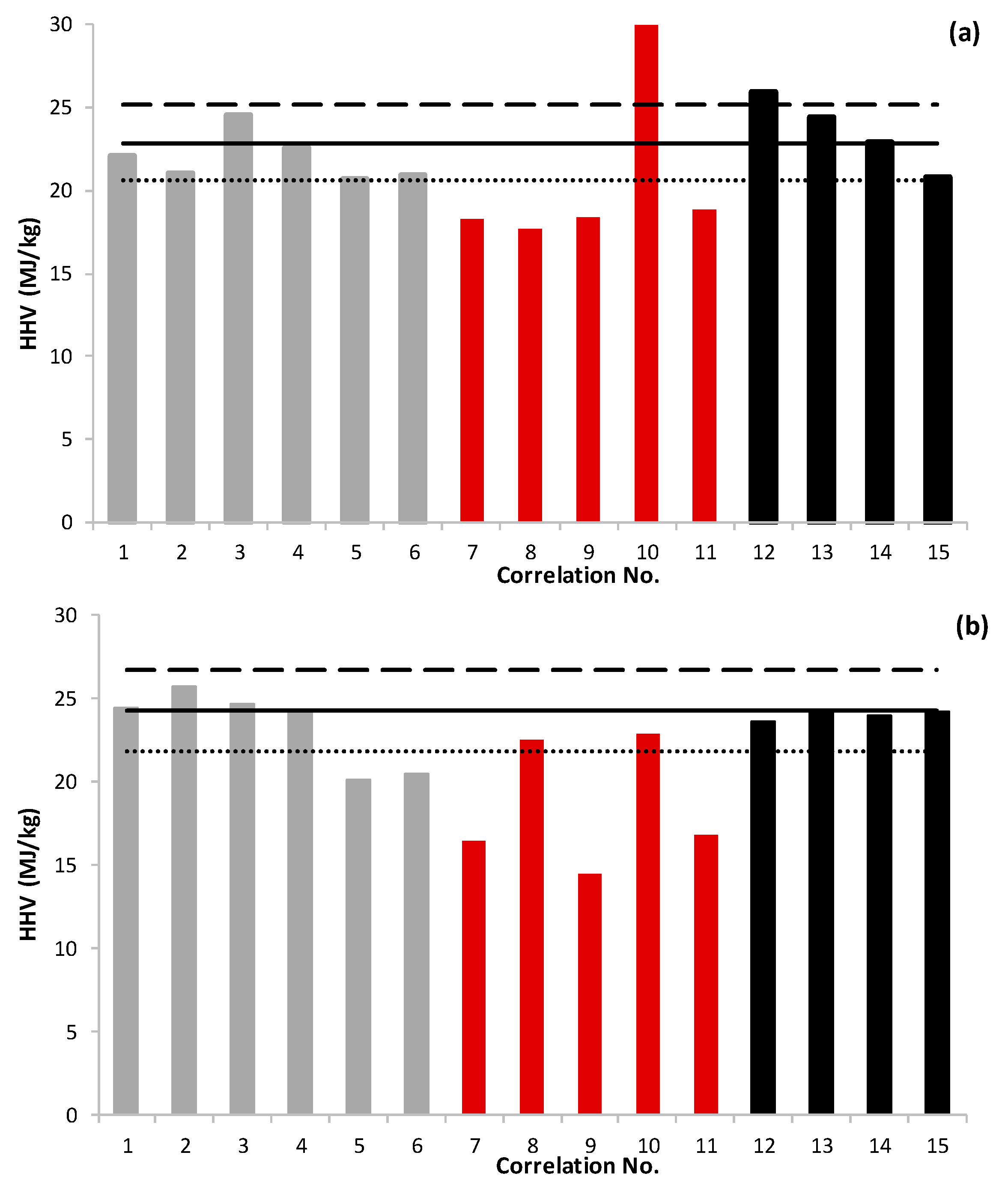
Figure 1. Estimated High Heating Value (HHV) for microalgae biomass (MB) (a) and BC (b) by correlations No. 1 to No. 15 listed in Table 1. For each material, the estimated HHV values are represented by verticals bars, the measured value is represented by a continuous horizontal line, the upper limit (measured HHV + 10%) is represented by a dashed line, and the lower limit (measured HHV − 10%) is marked with a dotted line.
Energies 12 02962 g001
Figure 2. Differential thermogravimetry (DTG) curves corresponding to the temperature programmed combustion of MB, BC and their blend (MB-BC) together with the weighted calculated curve corresponding to the blend (MB-BC (T)) at the different heating rates here used, namely 0.1 K/s (a), 0.2 K/s (b), 0.4 K/s (c), and 0.5 K/s (d).
Energies 12 02962 g002
Figure 3. Differential scanning calorimetric (DSC) curves corresponding to the temperature programmed combustion of MB, BC and their blend (MB-BC) together with the weighted calculated curve corresponding to the blend (MB-BC (T)) at the different heating rates here used, namely 0.1 K/s (a), 0.2 K/s (b), 0.4 K/s (c) and 0.5 K/s (d).
Energies 12 02962 g003
Figure 4. Thermogravimetry (TG) curves corresponding to the combustion of MB (a), BC (b), and MB-BC (c) at different heating rates. Conversion percentages (10, 20, 30, 40, 50, and 60%) have been marked by straight lines crossing experimental data.
Energies 12 02962 g004
Figure 5. Results on the combustion of MB (a,d), BC (b,e) and MB-BC (c,f) at the different heating rates together with fittings to the iso-conversional kinetic models of FWO (ac) and KAS (df). Note: The Y-axis of graphs was adjusted for the correct visualization of results.
Energies 12 02962 g005
Table 1. Correlations considered for the estimation of the high heating value (HHV).
No.ReferenceCORRELATIONOriginally Targeted Fuel
Based on Elemental Analysis
1Dulong [35] HHV ( MJ / kg ) = 0.763 + 0.301 [ C ] + 0.525 [ H ] + 0.064 [ O ] Biomass of any type and/or origin
2Tillman [36] HHV ( MJ / kg ) = 0.4373 [ C ] 1.6701 Biomass
3Abe [37] HHV ( MJ / kg ) = 0.3391 [ C ] + 1.4340 [ H ] 0.0970 [ O ] Biomass from florestal origin
4Demirbas et al. [38] HHV ( MJ / kg ) = 0.335 [ C ] + 1.423 [ H ] 0.154 [ O ] Lignocellulosic fuels
5Sheng and Azevedo [39] HHV ( MJ / kg ) = 1.3675 + 0.3137 [ C ] + 0.7009 [ H ] + 0.0318 [ O ] Biomass
6Yin [40] HHV ( MJ / kg ) = 0.2949 [ C ] + 0.8250 [ H ] Lignocellulosic fuels (agricultural by-products and wood)
Based on Proximate Analysis
7Jenkins and Ebeling [41] HHV ( MJ / kg ) = 26.601 0.304 [ Ash ] 0.082 [ VM ] Biomass of any type and/or origin
8Parikh et al. [42] HHV ( MJ / kg ) = 0.3536 [ FC ] + 0.1559 [ VM ] 0.0078 [ Ash ] Solid fuels
9Sheng and Azevedo [39] HHV ( MJ / kg ) = 3.0368 + 0.2218 [ VM ] + 0.2601 [ FC ] Biomass
10Majumder et al. [43] HHV ( MJ / kg ) = 10.81408 + 0.3133 ( [ VM ] + [ FC ] ) Coal
11Yin [40] HHV ( MJ / kg ) = 0.1905 [ VM ] + 0.2521 [ FC ] Lignocellulosic fuels (agricultural by-products and wood)
Based on both Elemental and Proximate Analysis
12Grabosky and Bain [44] HHV ( MJ / kg ) = 0.328 [ C ] + 1.4306 [ H ] 0.0237 [ N ] + 0.0929 [ S ] ( 1 [ Ash ] / 100 ) ( 40.11 [ H ] / [ C ] ) Biomass
13IGT [45] HHV ( MJ / kg ) = 0.341 [ C ] + 1.323 [ H ] + 0.068 [ S ] 0.0153 [ Ash ] 0.1194 ( [ O ] [ N ] ) Coal
14Channiwala and Parikh [46] HHV ( MJ / kg ) = 0.3491 [ C ] + 1.1783 [ H ] + 0.1005 [ S ] 0.1034 [ O ] 0.0151 [ N ] 0.0211 [ Ash ] Solid, liquid and gaseous fuels
15Sajdak et al. [47] HHV ( MJ / kg ) = 0.001 × ( 601.95 11.57 [ Ash ] 7.12 [ VM ] + 341.67 [ C ] + 1165.86 [ H ] 97.35 [ O ] 193.37 [ N ] + 110.36 [ S ] ) Biomass, biochar and coal
HHV: high heating value; [C]: carbon content; [H]: hydrogen content; [N]: nitrogen content; [S]: sulphur content; [O]: oxygen content; [FC]: fixed-carbon content; [VM]: volatile matter content; [Ash]: ash content; note: all values are expressed in wt% on dry basis.
Table 2. Proximate analysis, elemental analysis, and calorific values for the microalgae biomass (MB) and the bituminous coal (BC) used in this work.
PropertiesMBBC
Proximate Analysis (wt. %)
Moisture10.10.8
Volatiles (d.b.)78.28.2
Ashes (d.b.)6.231.1
FC* (d.b.)15.660.7
Elemental Analysis (wt. %, d.b.)
C52.062.7
H6.82.5
N10.71.3
S0.60.7
O*29.81.7
Calorific Analysis (MJ/kg, d.b.)
HHV22.924.3
FC: fixed-carbon; HHV: high heating value; d.b.: dry basis; * calculated by difference.
Table 3. Published results on the elemental and calorific analysis for different microalgae biomasses. For each case, the published High Heating Value (HHV) is shown together with the HHV estimated by correlations based on elemental analysis displayed in Table 1. Estimated HHVs that are within ± 10% the measured value are in bold.
ChlorellaChlorella vulgarisChlorella vulgarisChlorella vulgarisChlorella vulgarisChlorella vulgaris residueChlamydomonas reinhardtiiChlamydomonas reinhardtiiDunaliella tertiolectaNannocloropsis oceanicaNannocloropsis oceanica residueSpirulina platensisSpirulina platensisScenedesmus obliquus
ReferencesBabich
et al. [60]
Xu
et al. [61]
Xu
et al. [61]
Wang
et al. [62]
Kebelmann et al. [63]Wang
et al. [62]
Kebelmann
et al. [63]
Kebelmann
et al. [63]
Zou
et al. [64]
Chen
et al. [65]
Chen
et al. [65]
Jena and Das [66]Wu
et al. [67]
Chen
et al. [68]
Elemental Analysis (wt. %, d.b.)
C50.245.853.842.5143.945.045250.23950.0645.2446.1645.737.37
H7.35.67.726.776.26.887.47.35.377.466.557.147.715.8
N9.34.61.16.646.79.7910.711.11.997.5411.0710.5611.266.82
S--------0.620.470.560.740.75-
O33.238.73727.9543.329.4229.831.453.234.4736.5835.4425.6950.02
Calorific Analysis (MJ kg−1, d.b.)
HHV (measured)21.218.424.016.818.019.423.022.014.221.518.220.520.516.1
HHV (No. 1)21.516.622.719.116.019.922.921.911.321.518.219.522.012.0
HHV (No. 2)20.318.421.916.917.518.021.120.315.420.218.118.518.314.7
HHV (No. 3)24.219.825.721.419.622.325.424.415.824.321.222.524.116.1
HHV (No. 4)22.017.423.319.616.920.323.422.412.522.118.820.222.313.1
HHV (No. 5)20.518.222.117.618.118.521.120.516.320.718.619.219.216.0
HHV (No. 6)20.818.122.218.118.119.021.420.815.920.918.719.519.815.8
Table 4. Published results on the proximate, elemental and calorific analysis for different microalgae biomasses. For each case, the published High Heating Value (HHV) is shown together with the HHV estimated by correlations displayed in Table 1. Estimated HHVs that are within ± 10% the measured value are in bold.
ChlamydomonasChlorella sorokinianaChlorella sorokinianaChlorella vulgarisChlorella vulgarisIsochrysis galbanaNannochloropsis limneticaNannochloropsis gaditanaPhaeodactylum tricornutumSpirulina platensisScenedesmus almeriensis
ReferencesBui
et al. [69]
Bui
et al. [69]
Paniagua
et al. [59]
Chen
et al. [70]
Soria-Verdugo
et al. [71]
Soria-Verdugo
et al. [71]
Soria-Verdugo
et al. [71]
Soria-Verdugo
et al. [71]
Soria-Verdugo
et al. [71]
Soria-Verdugo
et al. [71]
López
et al. [72]
Proximate Analysis (wt. %, d.b., except for moisture (wt. %))
Moisture3.53.89.6-------5.4
Volatiles75.573.276.155.3776.2686.1384.0681.5662.181.4673.1
Ashes5.27.97.8310.2813.118.3110.529.1625.466.420
FC15.615.116.0734.3510.635.565.429.2812.4412.146.9
Elemental Analysis (wt. %, d.b.)
C40.3245.0747.947.8451.31743.64452.45352.80540.64749.72043.84
H7.387.646.46.417.6556.6208.0627.8036.6127.3386.08
N2.613.888.749.019.8975.4747.8838.2306.81311.5506.8
S..0.781.460.5730.8160.6170.5091.4460.6930.32
O44.535.5236.182517.44835.13620.46421.49319.02324.29922.96
Calorific Analysis (MJ kg−1, d.b.)
HHV (measured value)17.4120.418.721.922.919.9723.5124.519.3422.6220.91
HHV (No. 1)16.319.918.920.925.318.025.725.219.923.019.5
HHV (No. 2)16.018.019.319.320.817.421.321.416.120.117.5
HHV (No. 3)19.922.821.923.026.720.927.427.021.425.021.4
HHV (No. 4)17.220.519.621.325.418.625.925.520.123.419.8
HHV (No. 5)17.919.319.318.920.718.121.421.416.620.117.4
HHV (No. 6)18.019.619.419.421.418.322.122.017.420.717.9
HHV (No. 7)18.818.218.018.916.417.016.517.113.818.014.5
HHV (No. 8)17.216.717.520.715.515.314.915.913.916.913.7
HHV (No. 9)17.817.118.018.216.617.517.017.514.018.215.0
HHV (No. 10)29.828.829.430.028.530.129.329.924.130.925.3
HHV (No. 11)18.317.818.519.217.217.817.417.915.018.615.7
HHV (No. 12)--24.224.327.423.228.327.923.426.023.1
HHV (No. 13)--21.522.826.620.026.926.620.925.120.8
HHV (No. 14)--20.321.524.819.225.425.119.523.319.6
HHV (No. 15)--18.719.922.818.123.823.418.521.018.4
Table 5. Characteristic parameters of DTG combustion curves determined for microalgae biomass (MB), bituminous coal (BC) their blend (MB-CB).
B (K/s)Tv (K)Tm (K)Tf (K)DTGmax (%/s)
MB0.140054210310.0363
0.241054310400.0839
0.443355411000.1981
0.544055711200.2457
BC0.16407828740.0890
0.26578209300.1295
0.467186710350.1669
0.567587510500.1820
MB-BC0.16007819810.0873
0.26318239930.1281
0.464687010460.1645
0.565488510800.1844
Tv: onset temperature for volatile release and mass loss; Tm: temperature of maximum mass loss rate; Tf: final combustion temperature detected as mass stabilization; DTGmax: maximum mass loss rate.
Table 6. Characteristic parameters of DSC combustion curves determined for microalgae biomass (MB), bituminous coal (BC) their blend (MB-CB).
β (K/s)Ti (K)Tmax (K)Te (K)ΔH (kJ/g)
MB0.1450597100011.62
0.2460857101911.88
0.4470876110011.76
0.5475879116511.71
BC0.150078289313.87
0.250082096813.81
0.4500880104213.96
0.5500959108613.78
MB-BC0.146178295014.16
0.247082598014.12
0.4475875104614.15
0.5480964108014.11
Ti: onset temperature for energy release and peak integration; Tmax: temperature of maximum energy release during combustion; Te: temperature at the end of energy release during combustion; ΔH: enthalpy determined by integration of the heat release peak in the corresponding DSC combustion profile.
Table 7. Values of apparent activation energy (E, kJ/mol) determined for the combustion of MB, BC and their blend (MB-BC) at the considered conversion degrees (α), together with R2 corresponding to fittings in Figure 5.
αE (kJ/mol)
FWO
R2E (kJ/mol)
KAS
R2
MB0.11770.99951770.9954
0.22430.99782460.8958
0.33430.98823510.9322
0.41710.99531690.9587
0.51210.98641160.9971
0.61230.98441170.9588
197* ± 85 196* ± 90
BC0.11120.99951050.9950
0.21020.9978940.9971
0.3890.9882800.9973
0.4860.9953770.9926
0.5760.9864650.9974
0.6670.9844560.9925
89* ± 16 79* ± 18
MB-BC0.11520.99951470.9970
0.21180.99781110.9661
0.3980.9882900.9784
0.4910.9953820.9973
0.5800.9864680.9896
0.6770.9844670.9762
103* ± 28 94* ± 30
E* ± standard deviation from E values at the considered α.

