1. Introduction
In the last few years, an increasing number of smart meters has been deployed in smart city environments to monitor energy consumption in buildings. As a result, the collected data have increased at an exceptional rate, so that energy-related data are becoming big data. The plenitude of data provides a favorable circumstance to face valuable challenges and add intelligence in energy-related contexts. The knowledge discovery process applied to energy data can reveal hidden and actionable models and patterns, such as those characterising and predicting energy consumption, for different stakeholders, from energy managers, to analysts, and consumers.
In the last decades of the past century, data mining proved to be a valid solution for finding implicit, unknown, and useful information from very large datasets. The most popular data mining tasks include correlation analysis (e.g., association rules), prediction (e.g., classification, regression), and grouping similar data (e.g., clustering). Turning to the energy domain, the association rule mining and clustering allow unsupervised energy data exploration useful for summarizing usage patterns, while prediction algorithms enable energy consumption forecasting, which, in turn, paves the way for optimising heating distribution networks.
To effectively mine large collections of energy data, state-of-the-art data mining algorithms have often required crucial limitations to be addressed, such as those represented by computational resources. To this aim, scalable solutions have been devised in recent years, including wide-spread big data frameworks like Apache Hadoop [
1], and Apache Spark [
2]. However, the fast changing pace of the evolution of such distributed-computing technologies introduces two sources of problems: (i) on the one hand, they are not mature enough to be applied on a generic domain and still require some form of fine-tuning to fit the specific scenario; (ii) on the other hand, it is difficult to find suitable professional profiles trained on the latest advancements of such platforms. The proposed solution tries to accommodate the needs of energy experts and energy-provider companies of extracting data insights by exploiting machine-learning solutions which have much less stringent requirements on the professional skills of the data analysts.
The exploitation of big data platforms on energy-related data is of primary importance to extract useful, actionable, and previosuly unknown knowledge from data as well as to forecast future energy consumption. Thus, the analysis of energy data opens up a variety of interesting research issues across two research communities: energy and computer science. To design effective analytics tools, a considerable interaction between an energy scientist and a computer scientist is needed, with the former being mainly responsible for defining the end-goals and the assessment of extracted knowledge. Furthermore, a stronger involvement in the algorithm definition phase is beneficial to enrich the algorithm itself with domain-expert knowledge, such as physical laws and event models. The computer scientist tackles the task of selecting the right software platform, designing and developing efficient and effective algorithms, selecting the optimal analytic techniques to achieve the end-goals, with the right trade-off between quality of results and processing time or resources.
From the energy scientist’s point of view, a lot of research efforts should be devoted to analyzing, characterizing and understanding energy-related data to effectively support different interested users in the decision-making process, from energy managers and analysts, to end-users living in buildings. Different research challenges can be addressed, whose results have a great potential to influence the overall energy balance of our communities. From the computer scientist’s point of view, most of the technologies and algorithms related to big data processing and analytics have to be tailored to the specific features of the energy domain, such as heterogeneous sources and formats, variable data distributions, different abstraction levels, both fine and coarse grained, to effectively and efficiently support the knowledge extraction process.
This paper presents SPEC, a Scalable Predictor of PowEr Consumption. It provides a data mining engine for predicting the future power consumption over sliding time windows, specific to each building under exam. Different regression techniques and a classification method have been integrated into SPEC to build a model aimed at predicting the fine-grained power consumption at a time instant in the near future (i.e., with a limited time horizon): artificial neural networks, random forest regressor and ridge regression. furthermore, SPEC also includes the random forest classifier to forecast a power consumption level, instead of the fine-grained value. Each prediction model is tightly tailored to the specific building efficiency, by being trained only on power consumption historical data of the selected building. The SPEC methodology builds upon state-of-the-art distributed-computing solutions, namely, Apache Spark, which allows us to quickly analyze very large data collections. As a case study, SPEC has been validated on thermal power consumption collected in a major city in the North of Italy. Energy data have been enriched with meteorological open data. Experimental results, obtained on 12 buildings monitored every roughly five minutes for one year, demonstrate the effectiveness of the proposed methodology in predicting fine-grained power consumption with a limited average error and a good accuracy.
This paper is organized as follows. We first present the most used distributed and parallel frameworks, then the paper contribution is detailed. Next the description of the main building blocks of the SPEC engine is presented followed by the discussion of the experimental results yielded by the SPEC engine on real thermal power data. After the comparison of our approach with related works, we draw conclusions and presents future work.
2. Distributed Frameworks
The recent explosion in size of sensor-provided datasets has required the development of new distributed and parallel big data approaches, often replicated inside cloud-based services (e.g., platform-as-a-service tools) [
3]. In recent years, two frameworks have emerged: MapReduce [
4], as a programming paradigm, whose most popular implementation is provided by the Apache Hadoop platform, and Apache Spark [
2], a more real-time data-processing solution with improved performance. Both solutions allow programmers to focus on data-processing issues, disregarding low-level details of the physical data replication and distribution over a cluster of machines, and the corresponding network coordination. The first big data approach to crunch huge datasets was the MapReduce [
4] paradigm proposed by Google and then implemented in various software solutions, whose most popular is Apache Hadoop. MapReduce exploits data locality by moving the algorithm to the data instead of bringing the data to the algorithm, hence allowing each node of the distributed cluster to process local data only. To this aim, a proper storage system was developed, the Hadoop distributed file system (HDFS), which is probably the most widespread big data storage solution now, being compliant with almost all analytics software solutions.
More recently, the Apache Spark [
2] framework has been developed. Apache Spark is a general purpose in-memory distributed platform supporting many development languages. Although it maintains full compatibility with the MapReduce paradigm, it overcomes MapReduce limitations and has become the favorite platform for large-scale data analytics, by enabling distributed data caching within the nodes main memory, and reducing slow disk access.
Thanks to the availability of such distributed platforms, different libraries provide many open-sourced algorithms for machine learning. Mahout [
5], designed for Hadoop, is among the most widespread ones. It contains implementations in the data mining areas such as algorithms to address the cluster analysis, classification, and to support recommendation systems. All the current implementations are based on Hadoop MapReduce and has been exploited to support different data warehousing applications [
6,
7]. MLlib [
8], instead, is the Machine Learning library developed on Spark, and it is rapidly growing both in development and adoption (e.g., network traffic analysis [
9], social networks [
10]).
3. Contribution of This Work
The aim of this work is to provide to energy scientists a scalable engine to predict fine-grained power consumptions tailored to each specific building under exam. The proposed engine, named SPEC, is customized to efficiently manage energy data, and includes different data mining algorithms to forecast both real and categorical values of power consumption. Furthermore, self-evaluation metrics are included to help the domain experts in assessing the quality of the results obtained. SPEC is built upon state-of-the-art distributed-computing solutions: the current implementation exploits Apache Spark and is able to effectively scale to huge data collections. SPEC is designed to be helpful in various energy-related applications, such as heating and electricity consumptions. As a case study, the proposed engine has been validated to forecast heating consumption every five minutes on 12 buildings.
To analyze the robustness of the proposed engine, it has been tested in two peculiar conditions: (i) from 6:00 a.m. to 10:00 p.m., which includes both transient states with peak values and steady states with more stable consumption values, and (ii) from 5:00 p.m. to 10:00 p.m. with only the steady-state phase. As expected, the forecasting activity in the former case is more challenging.
The energy scientist can successfully exploit this engine without specific algorithm-related knowledge, by setting only the energy-relevant parameters to reach her goals. No development of ad-hoc procedures in a specific programming language is required. For example, energy scientists can choose between fine-grained (every five minutes) or coarse-grained (e.g., hour/day/week) measurement periods, they can select the best metrics to evaluate the results, and the corresponding time frame of interest (e.g., the complete day versus specific hours of the day). In addition to the simple exploitation of the proposed engine, knowing in advance the expected power consumption on a per-building basis can provide interesting knowledge to the energy providers, that can devise proper strategies to efficiently satisfy the energy demand for each building as well as for the overall network. Finally, predicting the power consumption allows both a more accurate energy network sizing, hence providing a more reliable provisioning service, and a more informed energy usage by end-users (customers), who can be encouraged with specific rewards to apply ad-hoc strategies to reduce power consumption during the transient phases, when the energy peak demand is critical to satisfy.
4. Related Work
Recently, energy-related data have gained traction as the focus of many machine-learning-enabled analysis. The wide diffusion of smart and tiny sensor devices has been throughly exploited to monitor indoor and outdoor environmental parameters supporting the collection of a large volume of measures with temporal and spatial information. The knowledge extraction process applied on these data collections discover an interesting subset of actionable knowledge to effectively support the decision making process of facility managers.
Many research contributions on energy-related data have been carried out for: (i) identifying the main factors that increase energy consumption (e.g., floors and room orientation [
11], location [
12], weather [
13]); (ii) characterizing consumption profiles among different users [
12,
14]; (iii) supporting data visualization and warning notification [
15]; (iv) efficient storing and retrieval operations based on NoSQL databases [
16];
A parallel research effort has been devoted to designing and developing systems providing innovative and widespread analytics services based on big data technologies. General purpose solutions [
17] have been proposed together with specific techniques tailored to a given application domain, such as thermal energy consumption [
18], residential energy use [
19], renewable energy [
20], air pollution levels [
21].
In [
22], various big data services based on a Hadoop large-scale energy-distribution platform have been analyzed. Authors conclude that most services goal is the energy efficiency improvement and the cost cut in heating maintenance and consumption. Other approaches contribute with algorithmic and technological solutions, such as clustering techniques and association rule mining: in these works, big data mining techniques are exploited both for prediction from historical data and for data exploration.
Similarly, different combinations of such techniques have also been successfully exploited in other domains, e.g., for scaling network data characterization [
23], and for social network data exploration [
10].
Addressing the wider energy-data management field, in [
24,
25] two different platforms and infrastructures for managing building-specific data from different smart-city sources are presented. In [
26,
27] different GIS-enabled frameworks for modelling urban district energy consumption are presented, with the former [
26] applied in New York city, and the latter [
27] in a North-western Italian city. However, they do not focus on energy consumption prediction but on classifying energy intensity in buildings [
26] and estimating space heating [
27].
Focusing on the energy forecasting techniques, in [
28], a predictor of energy consumption in buildings is proposed, consisting of four building blocks, from data acquisition to performance evaluation. In [
29], a thermal-load forecast approach combining multiple data-driven methods is presented, with experimental results on the next-day hourly load forecast.
In [
30] a prediction model for district energy consumption in medium (mothly) and long terms (yearly) is presented, based on an ensamble of three different data-mining techniques. In [
31] two data-driven thermal-load forecasting models are compared, one based on support vector machines, and another with two nonlinear autoregressive exogenous recurrent neural networks. In [
32], two heating distribution network substations in Changchun, China, were analyzed by means of data mining techniques. As a result, six operating states are identified in each heating season. Finally, in [
33] the predictions of three energy consumption linear models are compared on two Swedish cities. Forecasts target the next-day prediction and not the specific building prediction model. Overall, current state-of-the-art works do not address specifically the large-scale challenges while keeping focus on the fine-grained data-driven forecasts.
Similarly, research efforts have been devoted to characterizing energy consumption at a large scale [
34,
35] as well as energy efficiency based on real consumption data [
6] or estimated data [
36,
37]. The study presented in [
34] exploits a NoSQL technology to support the collection, storing and analysis of large volumes of energy-related data. In [
34], a datawarehouse-style solution targeting KPI computation based on the leading NoSQL database MongoDB [
38] has been proposed, exploiting the map-reduce approach. The proposed indicators consider the energy consumption during specific outdoor conditions (temperature range) to characterize the energy consumption of single buildings and groups of buildings in the same neighborhood. As a further step, a more advanced KPI computation approach is presented in [
6]. The work in [
6] presented the energy signature analysis (ESA) system. It is based on a big data methodology exploiting the map-reduce paradigm. It is able to characterize the building’s energy efficiency through the energy signature. The latter estimates the total heat loss coefficient of a building and it is computed by a linear regression of the power used for heating on the difference between the internal temperature and the external temperature. The building signature has been exploited to compute two KPIs: “(i) The intra-building KPI to compare latest observations with past energy demand in the same conditions, for example in a similar outdoor temperature and indoor temperature; and (ii) the inter-building KPI to rank the overall building performance with respect to nearby and similarly characterized buildings by considering spatial co-location, building size, and usage patterns (e.g., residential, office, public building)”. In [
39] an engine exploiting unsupervised machine learning approaches (clustering) and association rule mining is used to explore energy consumption in buildings.
Differently from the previously-mentioned research papers [
6,
34,
35,
39,
40], the current work presents an engine based on scalable machine learning approaches to forecast fine-grained power consumption. The previously-cited works focus on diverse targets and proposed different analytics approaches. They also describe a significantly dissimilar architecture, wheres the datawarehouse design is the same. In particular, no state-of-the-art solution provides a large-scale prediction with a fine-grained five minute resolution for each building. Specifically, the target of [
34,
39] is the characterization of the power consumption and the focus of [
6] is the energy efficiency characterization, to define a building ranking, whereas the present paper targets the predicting of sliding-windows power consumption. Furthermore, the methodologies proposed in [
6,
34] exploit the map-reduce paradigm, while this work exploits the more advanced and high-performing Apache Spark framework; and the approach proposed in [
35] does not include the forecasting data mining techniques exploited by the currently proposed methodology.
First attempts towards the prediction of fine-grained energy/power consumption over a sliding window have been proposed in [
41,
42]. The current paper significantly extends the study in [
41] by (i) providing a new algorithm to perform the regression task (i.e., the ridge regression model); (ii) including a new analytics method (i.e., classification approach) to address the prediction of power consumption labels through the random forest classifier; (iii) adapting the prediction models to a longer time frame, including the first hours of the morning when a large number of energy consumption spikes occur; (iv) introducing new and longer prediction horizons; (v) adding an exploitation use case of the proposed approach, based on a real-world district heating network, and (vi) providing a more in-depth and extensive experimental validation (almost three-fold expansion in experimental results).
5. The SPEC Engine
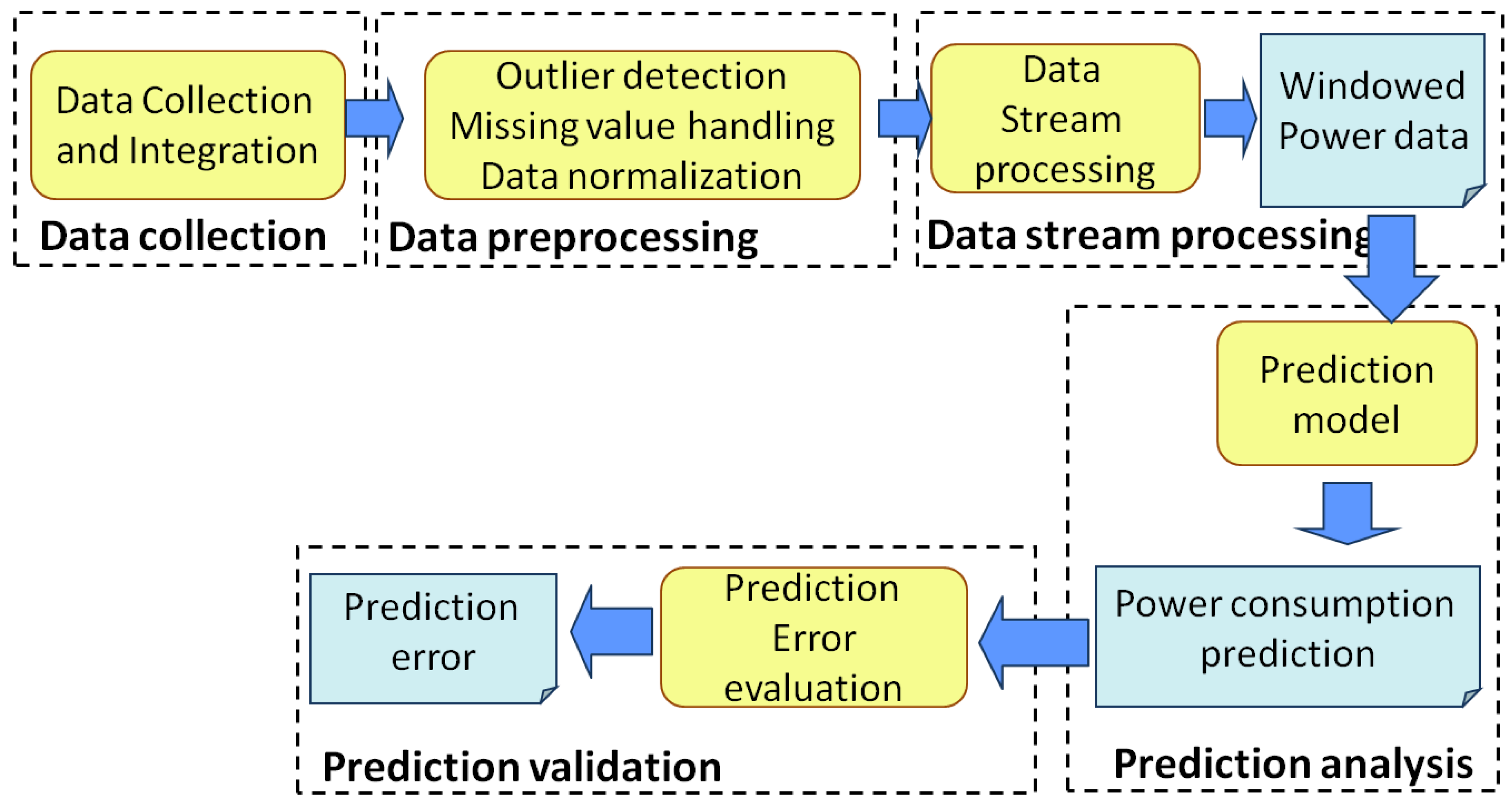
SPEC is a distributed analytics engine aimed at predicting fine-grained power consumption. Its architecture is presented in
Figure 1 and consists of different components, each addressing one of the main steps of the knowledge-extraction process. The scope of the current paper is to discuss SPEC performance and usage in the context of thermal energy consumption. To this aim, the dataset under analysis consists of thermal energy consumption data, collected every five minute from a large number of smart meters deployed in 12 buildings. As proposed in [
34], energy data are enriched with meteorological information, collected from open-data web services [
43]. Added meteorological information includes temperature, relative humidity, precipitation, wind direction, UV index , solar radiation and atmospheric pressure, as defined and provided by [
43]. The data collection and integration component is in charge of collecting energy consumption data and integrating meteorological information with the right temporal and geographical correlation. Since the focus is on thermal energy consumption in residential and office buildings, only measurements of the winter season are considered.
The other SPEC components are presented in the next subsections.
5.1. Data Preprocessing
The knowledge extraction process is a multi-step process typically starting with a preprocessing phase, whose aim is to smooth the effect of possibly unreliable measurements. SPEC preprocessing component provides three features which have been proved to be crucial in real-world sensor-provided energy data: (i) outlier detection and removal, (ii) missing value handling, and (iii) data normalization.
Outlier detection and removal. An outlier is a measurement that lies outside the expected range of values. It may occur either when the collected value does not fit the model under study or when faulty sensors provide unacceptable measurements for the phenomenon under analysis.
To detect outliers SPEC integrates the leverage measure. It is a coefficient based on the Mahalanobis distance to define whether a power consumption measurement (
) is different from the others. For each observation
, SPEC computes the leverage as proposed in [
44], as provided in Equation (
1):
where
N is the number of power consumption measurements, and the Mahalanobis distance, in our study, is computed as provided in Equation (
2):
where
is the mean of all energy samples, while
is the the total square difference between all samples in energy consumption and their mean. Only the observations
with a leverage value
greater than the
threshold are processed in the next analytics step. The
threshold value is computed as provided in Equation (
3):
where
K is the number of variables under analysis.
Missing value handling. Many strategies are available to address missing values. SPEC selects different approaches for different attributes, in particular for contextual data sources, such as unreliable weather data providers: (i) replacement with the daily average value or (ii) replacement with the hourly average value computed in the corresponding time of the previous week. The choice is mainly driven by the physical meaning of each attribute. Specifically, strategy (i) is exploited for rain precipitation and wind direction attributes, while strategy (ii) is applied to solar radiation and UV index attributes.
Data normalization is an important task required when differences in scale and measurement unit exist in the data under analysis. Specifically, the normalization technique allows preserving the original data distribution without affecting the relevance of the analytics results. SPEC integrates two normalization techniques: min-max and z-score. The typical state-of-the-practice approach is to iteratively perform different analysis sessions with different data normalization techniques to identify the strategy yielding better results.
5.2. Data Analysis
The core of the knowledge extraction process in SPEC consists of three building blocks: (i) data stream processing, (ii) prediction analysis, and (iii) prediction validation.
5.2.1. Data Stream Processing
In the buildings under analysis, a large volume of energy data is continuously collected since power consumption is monitored roughly every five. Due to the high volume of collected data, the SPEC engine performs the prediction over a sliding time window. Specifically, when a new power consumption measurement is collected from a building, a sliding window over its historical data stream is considered. This window contains a snapshot of the latest power consumption values of the building, together with correlated meteorological data. The time window size is a parameter () to be chosen depending on the temporal context of interest for the analysis: with short time windows, the evaluation is almost in real-time of the building’s consumption is performed based only on very recent measurements; instead, a very large time window includes many historical measurements.
5.2.2. Prediction Analysis
Many data mining algorithms are available for prediction purposes. Depending on the nature of the variable to predict, we can identify two broad classes of approaches: if we wish to predict future power consumption measurements as numerical values, then we focus on regression techniques; otherwise, if the prediction were a consumption level (such as high, mid, low), then a classification approach able to predict categorical values is required. SPEC addresses both requests by providing three regression techniques and a classification algorithm.
The prediction analysis component consists of two steps: (i) model building and (ii) prediction task. In (i) a model for the data under analysis is built by analyzing past power consumption together with meteorological data. Then the model is exploited to forecast the upcoming power consumption in (ii). Among the techniques available to our purposes there are regression-based methods, decision trees, naive Bayes approaches, neural networks, and support vector machines. Each technique employs different learning algorithms to build models from historical data. In SPEC a new data model is created for each time window. To self-assess the performance of the proposed prediction models, data are split into training and test sets. The former is used to build the model, whereas the latter to assess its quality.
For the regression purposes, i.e., the prediction of a real value of power consumption, SPEC provides the following techniques: ridge regression (RR), random forest regression (RFR), and artificial neural networks (ANN). While the latter two techniques have been widely and successfully exploited in many different applications , the former was included to provide better insights to the energy-provider company. The selected techniques are briefly presented in the following, specifically focusing on the Apache Spark implementation.
Ridge regression (RR) builds a model based on the linear dependency among data under analysis. Given a set of input features expressed through a n-dimensional vector x = [] and a target variable representing the objective of the prediction, the algorithm builds a regression model with L2-regularization using stochastic gradient descent that provides a good estimation of the value of y.
Random forest regressor (RFR) is an ensemble learning method that can be used for regression. Given a training set with known predictions, a group (forest) of decision trees is created as a model. The forest approach reduces the risk of overfitting. In MLlib [
8], the RFR algorithm creates different trees during the training phase by generating randomness and minimizing overfitting. The randomness is introduced by (i) performing
N sub-sampling of the training set (i.e., bootstrapping), (ii) considering different random subsets of input variables. Thus, a parallel execution of the training step is possible. During the application of the model, the single class labels produced by each tree are aggregated and a global result is computed. Labels are replaced by real values in case of regression problems.
The building of each decision tree is a top-down process: an attribute test condition is chosen at each step so that it best splits the records. To this aim, the Gini index can be exploited. Each node in the tree represents a test on an attribute, being each branch, descending from a node, a range of possible values for that attribute. Leaves represent values of the target attribute. This allows to partition the sample space depending on the test conditions of the different attributes at each node.
To generate a prediction, the tree is visited top-down, following the tests in each node, and branching down to a resulting leaf.
Artificial neural networks (ANN) exploited in SPEC are multi-layer networks without restrictions (the source code has been downloaded from
https://github.com/yannart/Scala-Neural-Network). They include an input layer,
n hidden layers, and an output layer. Each node in a layer takes as input a weighted sum of the outputs of all the nodes in the previous layer, and it applies a nonlinear activation function to the weighted input. The network is trained with back-propagation and learns by iteratively processing the set of training data records: weights in the network nodes are backward updated to minimize the mean squared prediction error.
Among the available techniques suited to the classification problem (i.e., the prediction of a categorical value such as a range of values of power consumption) SPEC provides the random forest classifier (RFC).
The random forest classifier (RFR) is a technique very similar to the random forest regressor. It is an ensemble learning method based on a pool of trees. Differently from the regressor, the predictions are categorical, such as high, mid, or low energy consumption levels. Each level can be associated to a specific range of real consumption values. There is virtually no limit in the number of different categorical values, however, such techniques typically work well with a low number of classes (i.e., different predicted categories), in the order of tens at most. They are useful because often it is not the precise real value to be of interest, but its level in terms of meaningfulness for the phenomena under study. Hopefully, grouping contiguous values into the same level (i.e., discretization into category), helps in improving accuracy results. Technically, the difference with the regressor is in the the final predicted value, which cannot be computed as the average of the single tree predictions, but a majority voting approach is used: the category voted by the largest number of trees is selected as the final result of the forest classifier.
5.2.3. Prediction Validation
This component evaluates the ability of the SPEC engine to correctly predict the energy consumption of a building. To this aim, SPEC integrates three metrics to evaluate the quality of regression-based models and one metric for the classification-based models: (i) mean absolute percentage error (MAPE), (ii) weighted absolute percentage error (WAPE), and (iii) symmetric mean absolute percentage error (SMAPE), whose formulas are reported in the following, are the regression metrics, whereas the accuracy is used for the classification model. Accuracy is the ratio of the correct predictions with respect to the overall number of predictions. The metrics are provided in the following Equations (
4)–(
6).
In all formulas, is the actual energy consumption at time while is the corresponding predicted value.
MAPE, or mean absolute percentage deviation (MAPD), can evaluate a predictor quality. However, since MAPE is a percentage, it might be less suitable for energy predictions because of its sensitivity to low absolute values: given the same absolute error, MAPE may be very large in presence of low consumption values, while it might hide errors when the absolute consumption is very high. The WAPE and SMAPE metrics have been proposed to address this issue. WAPE suffers from not having a specific meaning as an error on the single prediction but only on all the forecasts, while SMAPE is able to correctly model the prediction error for each forecast individually. The only drawback of SMAPE is that it is not symmetric. Thus, overestimated forecasts and underestimated forecasts do not have the same impact. Specifically, for the same value of prediction error, the underestimated forecast has a greater impact on the overall SMAPE value. Since each metric has benefits and drawbacks, SPEC provides them all to allow the energy analyst to select the best one for her goals.
6. Experimental Results
We tested the efficiency of SPEC by performing different experimental sessions on a real dataset, including power consumption data collected from 12 residential buildings. Measurements are collected over a full winter period in Italy, from October 15th to April 15th. Energy data have been enriched with meteorological information collected from the weather underground web service (the weather underground web service gathers meteorological data from personal weather stations (PWS) registered by users) [
43].
The experiments reported in the paper target a subset of the overall district heating buildings, specifically those buildings for which the full historical datasets of real-world data measurements were available.
The datasets have been stored in a Hadoop cluster available at our University, based on the Cloudera Distribution of Apache Hadoop, version 6.1.0. All experiments have been performed on our cluster, which has 8 worker nodes, and runs Apache Hadoop 3.0.0 and Spark 2.4. The current implementation of SPEC is a project developed in Scala exploiting the Apache Spark framework.
Input variables are: time, date, temperature, humidity, precipitations, pressure, dew point, wind direction, and energy consumption, in the configured time window. The target of the prediction task is the upcoming energy consumption in the near future. For the results reported in this study, the SPEC engine configuration featured the normalization and outlier detection through the min-Max technique and the Leverage approach, respectively; the time window size () has been set to three samples (i.e., roughly 15 min). A parameter grid search has been performed to identify values for algorithm parameters. To configure the ridge regression algorithm in MLlib, the following parameters have been set: intercept = false, numIterations = 100, regParam = 0.01, stepSize = 1.0. For both the Random Forest Regressor and Classifier in MLlib, the parameters were: numTrees = 20, featureSubsetStrategy = all, impurity = variance, maxDepth = 4, maxBins = 100. The ANN regressor has been used with perceptronInputNum = 9 and neuronLayerNum = Array [10, 2, 1].
Experimental results targeted the five minute prediction capability. To this aim, we evaluated the prediction error for all algorithms and all buildings separately. The prediction error has been computed as the averaged error of all predictions in the whole (winter) period. To perform the prediction task we considered two different time frames: (i) the complete day, from 6:00 a.m. to 10:00 p.m.; (ii) the afternoon/evening only, from 5:00 p.m. to 10:00 p.m. The former time frame includes both transient and steady-state phases, thus the prediction is more challenging: values were characterized by large variability and spikes. The second time frame includes typical steady-state phases, with more stable consumption values, hence the prediction task is expected to be easier.
Table 1,
Table 2 and
Table 3 report the MAPE, WAPE, SMAPE values for each monitored building obtained through the ridge regression (RR), artificial neural networks (ANN), and the Random Forest Regression (RFR) models respectively.
Table 1,
Table 2 and
Table 3 focus on the 5–10 p.m. time frame, whereas
Table 4,
Table 5 and
Table 6 report results of the whole day.
All three regression models yield good results by analyzing consumption values in the 5–10 p.m. time frame. Both RR and ANN models present limited errors: ANN has a MAPE of 6–19%, a WAPE of 6–10%, and a SMAPE of 3–5% as reported in
Table 2. Such results are very similar to the ones yielded by RR in
Table 1). Also the performances of RFR are quite good, although slightly worse than both RR and ANN models: it has a MAPE of 9–20%, a WAPE of 9–14%, and a SMAPE of 5–7% as reported in
Table 3).
As expected, errors yielded by SPEC models worsen when the prediction task is performed for the whole day. As shown in
Table 4,
Table 5 and
Table 6, on average ANN models reach the best results, with an average prediction error lower than both RR and RFR. Results of RFR are better than RR, although slightly worse than ANN.
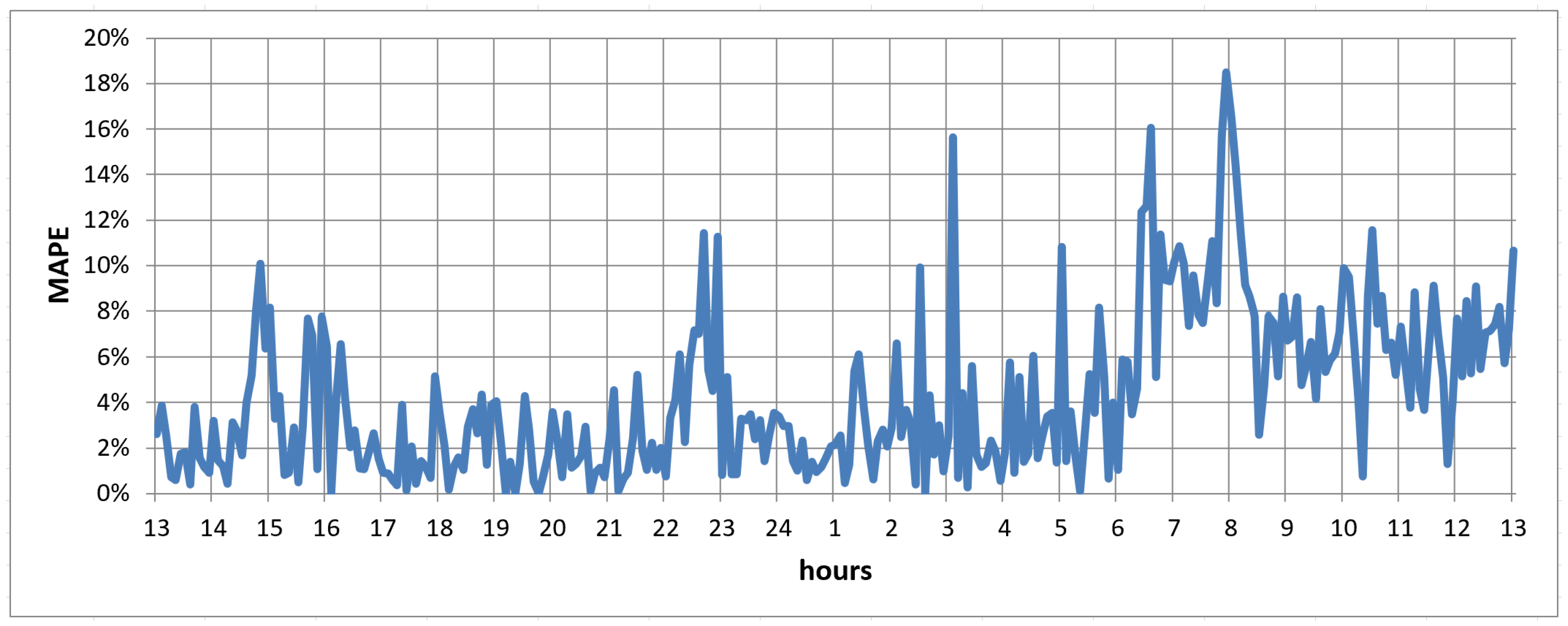
Since the ANN model yielded the lowest errors and on average achieved better results than both RR and RFR on all time frames (i.e., 6 a.m.–10 p.m. and 5–10 p.m.), we analyzed in more details the error trend yielded by ANN in a given day for a representative building, as reported in
Figure 2. Building no. 7 is selected as representatives because its consumption time series include multiple peaks. In all cases, the ANN models are able to predict values following the trend of the actual time series, although the error significantly increases for peaks in energy consumption, such as during the early morning (e.g., 7–8 a.m).
We experimentally evaluated the performance of the random forest classifier provided by SPEC. To perform the categorical classification task, the power consumption values per unit of volume have been discretized in six fixed-size bins as in [
39]: two bins until 15.5 KW/m
(off until 0.05 KW/m
, low until 15.5 KW/m
), a bin each 10 KW/m
for values until 35.5 (medium consumption until 25.5, high consumption until 35.5) and an additional bin for values exceeding 35.5 KW/m
.
Table 7 reports the accuracy yielded on the 12 buildings under analysis for both the complete day and afternoon/evening time frames. In both cases the classifier achieved good accuracy values: they are in the range from 81–91% when analyzing all collected values (6 a.m.–10 p.m.), and in the range 89–98% (except for building no. 1) on the afternoon/evening time frame.
Regarding the prediction horizon, we analyze the performance in terms of MAPE, WAPE, and SMAPE of the top-performing approach, i.e., ANN, with longer prediction horizons, specifically 30, 45, and 60 min, as reported in
Table 8. The selected 5 buildings are those presenting no missing values, hence not requiring any pre-processing. Such results are compared with two naive techniques: (NAIVE 1) previous-value predictor and (NAIVE 2) same-time previous-day predictor.
Improvements in terms of prediction error reduction of the artificial neural network model over the two selected naive approaches for a 30-min prediction horizon in the time frame 6 a.m.–10 p.m. are reported in
Table 9. The results for prediction horizons of 45 and 60 min are reported in
Table 10 and
Table 11 respectively.
The proposed approach always yields to better predictions (i.e., with lower errors) with respect to the NAIVE 2 approach. Similar results are also reported with respect to NAIVE 1 apart from a single exception (SMAPE for building B2). Improvements for building B1 are higher with respect to NAIVE 1 and lower with respect to NAIVE 2, whereas the converse is true for the remaining buildings. This is due to the different usage pattern of residential versus office/public buildings.
Considering the performance of the ANN model on longer prediction horizons, we notice that errors for 30, 45, and 60 min are lower than five minute forecasts. If the energy provider operations can benefit from a 5-min prediction horizon, this is proved to be a more challenging task than 30–60 min horizons. Changing the prediction horizon from 30 to 60 min does not affect significantly the error rates.
Statistical significance of the difference in the values in
Table 9,
Table 10 and
Table 11 have been computed with the Student
t-test for the MAPE metric. Bold values indicate that the
t-test has been passed for a
p-value of 0.05. We notice that improvements reported for the 60-min horizon are statistically significant for all buildings, and they would be significant also for lower
p-values, such as 0.01. On the contrary, the shorter the horizon, the less significant the improvements: for the 45-min horizon, only three buildings out of five pass the
t-test with
p-value 0.05, whereas all 5 would pass the
t-test for
p-value 0.10. For the 30-min horizon, again three out of five buildings pass the
t-test with
p-value 0.05, however the remaining two buildings would require a
p-value larger than 0.10.
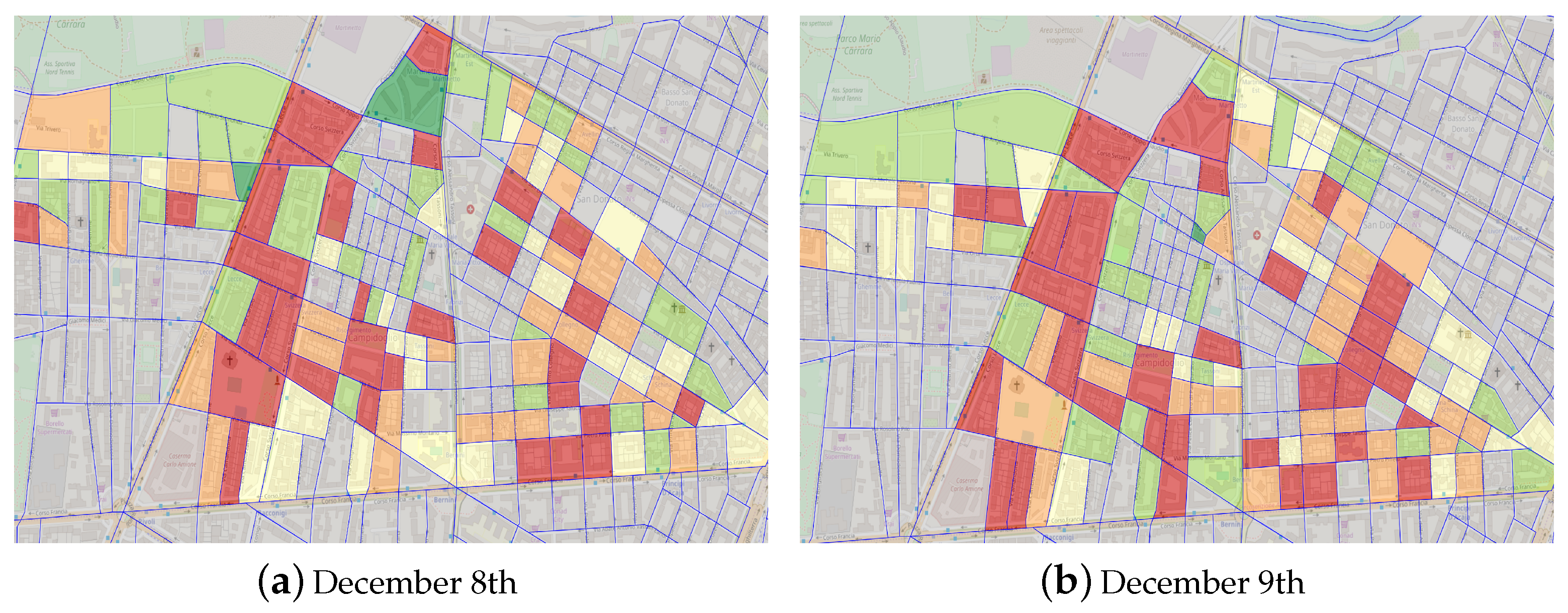
Finally, we present a sample of how the proposed work could be exploited in a real-world district-heating distribution network. The goal of the solution is to be a tool directly available to energy experts and energy-providing company management to support their decisions in the strategic design and expansion plan of the district heating networks, besides the day-to-day operations. In
Figure 3, a district map of building consumption levels with real experimental data is presented for two different days, December 8th in
Figure 3a and December 9th in
Figure 3b. Each of the five consumption levels is a percentage range of the top consumption among the overall population for that day, and it is associated with a color from green (0–20%) to red (80–100%). The aim is to analyze the total consumption of each neighborhood in the district under exam, hence grouping together the single buildings but keeping a fine-grained spatial resolution. While such a map can be produced for any prediction horizon, the presented results describe a whole day consumption, considering that December 8th is a national holiday. Specific patterns emerge for residential versus office/public buildings; for instance, the two neighborhoods at the top-centre of the map had opposite behaviors: the lower one is green (0–20%) during the national holiday (
Figure 3a) and red (80–100%) on the next day (
Figure 3b), and indeed it is a neighborhood of office buildings. On the contrary, the upper neighborhood is red (80–100%) during the national holiday (
Figure 3a), and light green (20–40%) during the next day, hence showing the behavior of a residential building with most people working out of home.
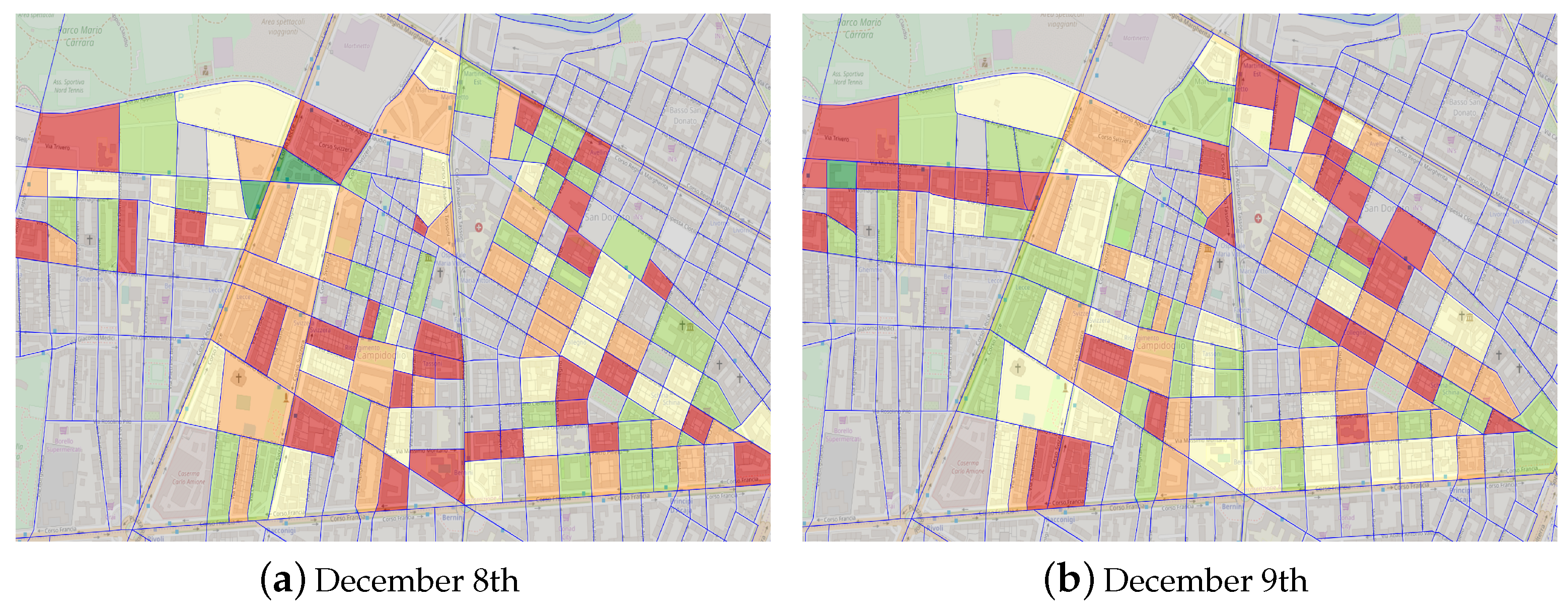
The map reported in
Figure 4 similarly provides the average consumption per m
, hence being useful to estimate the energy efficiency of the buildings. It is interesting to note that during the national holiday, even if the previously analyzed office neighborhood was green (0–20%) in total consumption (
Figure 3a), it is orange (60–80%) in average consumption (
Figure 4a), hence being poorly efficient when using low total energy. On the contrary, it has a very high energy efficiency on December 9th (
Figure 4b) with a light-green level (20–40%), when it is a top consuming neighborhood (red level 80–100%, (
Figure 3b).


