Article

Life Cycle Assessment of New High Concentration Photovoltaic (HCPV) Modules and Multi-Junction Cells

1
CYCLECO, 18 Avenue Roger Salengro, 01500 Ambérieu-en Bugey, France
2
SIE-GE Ecole Polytechnique Fédérale de Lausanne (EPFL), 1015 Lausanne, Switzerland
*
Author to whom correspondence should be addressed.
Energies 2019, 12(15), 2916; https://doi.org/10.3390/en12152916
Submission received: 28 May 2019 / Revised: 12 July 2019 / Accepted: 17 July 2019 / Published: 29 July 2019

Abstract

:
Worldwide electricity consumption increases by 2.6% each year. Greenhouse gas emissions due to electricity production raise by 2.1% per year on average. The development of efficient low-carbon-footprint renewable energy systems is urgently needed. CPVMatch investigates the feasibility of mirror or lens-based High Concentration Photovoltaic (HCPV) systems. Thanks to innovative four junction solar cells, new glass coatings, Position Sensitive Detectors (PSD), and DC/DC converters, it is possible to reach concentration levels higher than 800× and a module efficiency between 36.7% and 41.6%. From a circular economy’s standpoint, the use of concentration technologies lowers the need in active material, increases recyclability, and reduces the risk of material contamination. By using the Life Cycle Assessment method, it is demonstrated that HCPV presents a carbon footprint ranking between 16.4 and 18.4 g CO2-eq/kWh. A comparison with other energy means for 16 impact categories including primary energy demand and particle emissions points out that the environmental footprint of HCPV is typically 50 to 100 times lower than fossil fuels footprint. HCPV’s footprint is also three times lower than that of crystalline photovoltaic solutions and is close to the environmental performance of wind power and hydropower.

Graphical Abstract

1. Introduction

The total amount of consumed energy on earth has raised by 13.7% between 2007 and 2016 [1]. During this time period, electricity production has continuously risen, with an annual increase of 2.6% on average due to the increase of electricity share of 1.8% in the total energy demand [1]. In the end, electricity production from burning fossil fuel increases annually by 2.1% on average. Data from the year of 2016 indicates that 16 million GWh of electricity came from fossil fuels (which represented 65.06% of the electricity mix) [1]. In the last 10 years, the amount of fossil fuels burnt to electricity has been growing. Thus, despite the increase of the share of renewable energy in the world’s electricity mix (0.55% per year for 10 years), the overall carbon footprint of electricity production on a global level has been increasing continuously.
At the same time, world temperature is increasing because of greenhouse gas (GHG) emissions. Consumed Energy is responsible for 65% of GHG emissions. Amongst it, electricity is responsible for 36.8% of these emissions in 2015 (Appendix A). Despite the efforts of numerous states engaged in international agreements such as the Paris Agreement during COP21, the carbon footprint of world electricity production has grown by 19% between 2007 and 2016. Concerning the environment, global warming is clearly a major challenge as far as future electricity production is concerned. Nevertheless, it is just one of the issues linked to the burning of fossils fuels. Beyond this issue, our society is facing several environmental challenges which are reflected by other impact categories. High exposure to small particles (PM2.5) on earth represents the main global health disease, causing 4.6 million deaths [2], corresponding to 8% of all deaths worldwide. Other environmental issues are associated with the large deployment of renewable energies, especially solar energy. Land use, for example, is a tricky issue. Energy production from the sun requires large surfaces, because conversion efficiency of existing technologies for solar photovoltaics is too small to satisfy the needs of developed countries [3,4]. However, concurrently, the world population requires more and more cultivated area for food production. This competition for land use shall be handled using a multi-criteria approach, considering this impact category. Moreover, threats to biodiversity is also a crucial issue in our society. It is now largely accepted that human activities are causing the sixth mass extinction of species [5,6]. Part of these impacts are from direct emissions in the environment, such as toxic or eutrophying substances. Impact categories such as ecotoxicity [7,8,9], eutrophication [10], and acidification [11,12] enable addressing the impact on aquatic biodiversity [10,13].
The deployment of renewable energy is currently based on several potential resources for energy production, including wind, hydropower, biomass, geothermal, and solar energy. Amongst these, wind power, hydropower, and solar power are particularly promising. Hydropower presents a small carbon footprint [14,15] and allows a flexible production over time. Nevertheless, production facilities are often not located close to areas of important electricity needs and their exploitation for energy is not easily compatible with other water uses or ecological objectives. Wind power also presents a small carbon footprint [16] and is largely available. Nevertheless, wind power production is not flexible, has low predictability, and requires an important electric network. Concerning solar energy, availability is high; the sun is almost everywhere and is not facing ecological issues. Nevertheless, the carbon footprint is typically higher than other types of renewable electricity, and competition with other land uses has to be managed. Its huge potential and fast growth in the last decades are promising [17,18] and suggest exploration of new technologies which reduce both carbon footprint and land occupation. Solar energy is indeed a land-intensive technology [19,20]. This important impact on land occupation is a matter of concern for European countries facing strong pressure on the use of available area. Solar energy in competition with agriculture and ecosystem equilibrium can limit PV growth in the next decades [21].
Given a growing energy demand and the pressure on land resources, concentrating solar energy is a promising solution. Concentrated solar power (CSP) plants have been investigated through several case studies [22,23,24], but further developments—mainly on the conversion efficiency from thermal to electrical energy—must be carried out. This solution is limited by its high technological requirement and a complex infrastructure. This limits the installation of CSP plants to the solar belt area. An alternative technology with concentration is explored with solar Concentrated Photovoltaics (CPV) and High Concentrated Photovoltaics (HCPV) technologies. Recent researches are focusing on concentration ratio, cell, and module efficiency based on the improvement of multi-junction cells and modules. These parameters are evaluated within the framework of the project with three technologies. One mirror-based and two lens-based HCPV modules [25,26] mounted with III-V four-junction cells [27], working at a concentration of 800× and 320×, respectively. These technologies are assessed in terms of environmental performance by using the Life Cycle Assessment (LCA) method. The purpose of this article is to assess the environmental performance of HCPV technologies and to identify the potential environmental benefits/limitations of this technology.

2. High Concentration Photovoltaic Technologies

Several LCA studies are already available for assessing CPV and HCPV technologies and plants. These studies specially focus on carbon footprint and are often based on very different assumptions. A study relating to a plant in Morocco [28] reports, for example, a carbon footprint of 53.3 g CO2-eq/kWh for a 1.008 MW HCPV plant. In this case, III-V multi-junction solar cells are mounted with polymethylmethacrylate (PMMA) Fresnel lenses on modules. Raw material extraction and component manufacturing, considering steel and aluminum, contributed the most to the impact. The ‘Apollon CPV module’ LCA evaluation revealed that aluminum and electronic components were the most impacting processes [29]. The carbon footprint of the system mounted on a two-axis tracker in Catania was estimated at 20 g CO2-eq/kWh.
De Wild-Scholten [30] determined greenhouse gas (GHG) emissions for a SolarTec based on a Fresnel lens and CPower mounted with a mirror that concentrates the light on monocrystalline silicon and III-V solar cells. They reported GHG emissions of 35 g CO2-eq/kWh for a CPower module on an optimized tracker operating in Catania, Sicily. However, in the same study and under the same conditions, a SolarTec module presents an actual performance of 42 g CO2-eq/kWh.
The nature of the consumed electricity mix for HCPV module manufacturing highly influences the climate change impact. Fthenakis V.M. [31] reported 27 g CO2-eq/kWh over a 30 year operation for the Ammonix 7700 26-kW HCPV system equipped with single-crystal Si cells installed in Phoenix, AZ, USA. The tracker and the module accounted for the largest part of its life cycle energy use and emissions. A previous study in 2007 [32] made very similar conclusions. However, it reported 38 g CO2-eq/kWh for the 24 kW-Ammonix concentrator PV system with single-crystal Si cells. Also, a study presenting FLATCON results, with a HCPV system, also presented similar results with 30 CO2-eq/kWh [33].
A novel wafer-bonded four-junction solar cell was developed for better spectral matching by European research institutes and industrial partners using new processes and materials. This III-V multi-junction solar cell [GaInP/GaAs//GaInAs/Ge] presents a high potential in matching the entire spectral light. Those semiconductor materials allow the absorbance of a larger range of wavelengths. Added nano-structured coatings [34] improved light trapping and therefore solar cell efficiency. Catching more solar energy with an identical surface is then possible. DC power optimizers [35] present higher conversion efficiencies when facing mismatch issues due to misalignment between the optics and receivers. In high concentrating photovoltaic (HCPV) systems, lenses [32] or mirrors can be used to concentrate solar radiation on these multi-junction cells. Higher efficiency of modules was recorded at 38.9% [36]. These systems can reach a concentration higher than 800× with solar cell efficiency of 44%, potentially reaching 48% in the coming years. Light concentration through optics (mirrors or lenses) allows the use of a smaller surface of active materials; nevertheless, such manufacturing processes are more energy-demanding and require higher quality materials. It is therefore interesting to assess the impact of the production system and to compare it with existing technologies.

3. Methods

3.1. Research Methodology

The research work was required to fulfill ISO 14040-44 standard requirements and is expected to provide responses to the project CPVMatch supported by the European Framework Programme for Research (H2020). This project involved several industry partners who actively contributed to data collection. Data collection aimed at enabling a transparent appraisal. Partners provided exhaustive inventory data coherent with industry practices. In spite of the iterative efforts in collecting data and the continuous collaboration with partners, it was sometimes necessary to fill in data gaps. In that case, literature data was used after being validated by partners. Irradiance was another key point; the calculation of Direct Normal Irradiance with a two-axis tracker stems from PVGIS’s website (2016). HCPVs aim at being produced in Europe, therefore the environmental footprint of electricity mixes, was fully modeled using recent statistics [37]. We modeled transportation steps based on expert knowledge, and details are presented in the life cycle inventory section. The two-axis tracker inventory is taken directly from the literature [38]. All life cycle inventory data is directly accessible either in the references or in the supplementary materials. A sensitive point concerns the life expectancy of the components of the HCPV modules. For the HCPV module itself, the life expectancy is 30 years (as well as for the two-axis tracker), while the inverters’ life expectancy is 10 years. Finally, the End-Of-Life (EOL) inventory data is completed with existing publications, as mentioned in the life cycle inventory section.

3.2. Life Cycle Assessment Presentation

Life Cycle Assessment (LCA) considers the entire life cycle of a product, from raw material extraction to the end-of-life, including energy consumption, material production, manufacturing, use, and end-of-life treatment. Based on this holistic vision of the product, technical data related to material and processes are converted in environmental performances in a multi-criteria analysis covering very diverse impact categories. LCA is well adapted for products with a long lifespan and used manufactured components in different countries. Indeed the impacts reflecting the environmental performances of the products are integrated over time and averaged over space [39].
An LCA study can be divided into four steps as described in the ISO 14040-44 standard [40,41]. The first step concerns the objectives of the study and the target audience. Then, it should define the scope and goal definition with the function, the functional unit, and the description of the system’s boundaries. This steps also presents all the assumptions used to model the system. The second step covers the life cycle inventory. It is necessary to identify all inputs and outputs linked to the functional unit. Assumptions related to primary and secondary data should be clearly stated for transparency. The third step concerns the life cycle impact assessment. It allows the conversion of elementary to flow (the list of all the resources used and all the emissions in the air, water, and soil) into impact results for each of the considered impact categories. Finally, the interpretation step is required. At this stage, all assumptions and modeling decisions which can affect the conclusions are tested in order to check how far the corresponding data question the conclusion. LCA is an iterative work; indeed, the interpretation can lead to the revision of assumptions and the recalculation of the results.
The methodological framework used for the LCA study is based on ISO 14040-44 standards. The International Reference for Life Cycle Data (ILCD) handbook [42] and the Product Environmental Footprint (PEF) guidance version 6.3 [43] are also considered. The ILCD Midpoint 2011 methodology was used to quantify the potential environmental impacts of the three HCPV scenarios. SimaPro 9.0.0 was used for the calculations.

4. Scope and Goal Definition

4.1. Function and Functional Unit

The functional unit describes the function performed by the system. The functional unit allows a comparison of different scenarios. Impact results are divided by the electrical energy which is exported to the grid during the system’s lifespan.
As mentioned by Udo de Haes [44], the main specificity of the LCA is the notion of functional unit. This requires describing the service, as well as the function, and comparing the scenarios on a reference unit related to this function also called “Functional Unit”. Several LCA studies on PV systems [45,46] defined their functional unit as 1 kWp of modules. Nevertheless, a conversion into energy unit (kWh) considering the solar irradiation is necessary to compare it with other electricity sources or other studies. As what is done in numerous studies such as [28,30,31,47,48,49], the functional unit is the production of 1 kWh of electricity exported to the grid.
The functional unit refers to the production of 1 kWh of electricity exported to the grid by a CPV module mounted on a two-axis tracker installed in Catania, Sicily, Italy during 30 years.

4.2. The Three Different Scenarios Under Study

In this article, three different concentrating photovoltaic modules are compared, each one using different concentrating technologies. One mirror-based module, one Fresnel lens, and one Achromalens HCPV module. Their characteristics are presented in the Table 1.
The two-axis tracker may have a different number of modules mounted depending on the technology. The system uses novel four-junction cells (FJCs) [GaInP/GaAs//GaInAs/Ge] grown on a Germanium substrate.

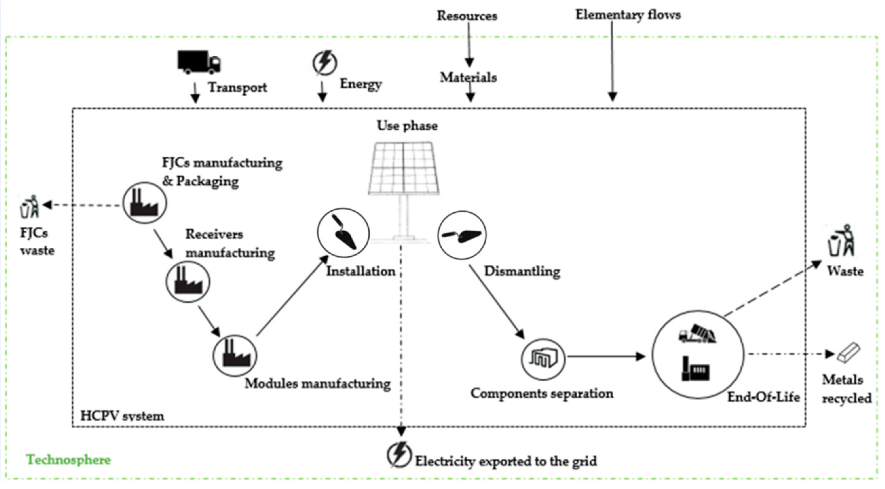
4.3. System Boundaries

We collected the detailed inventory data for the component manufacturing. It includes energy and heat consumption, as well as transportation and elementary flows into the environment. Figure 1 presents the perimeter of the study.
Concerning the infrastructure, the factory is included but not the machines. Direct emissions, waste, and packaging are not included at all life cycle stages except for the CPV wafer packaging.
At the end-of-life, the HCPV system is dismantled. Foundation of the tracker is not included at the end-of-life. Then, each component is allocated to a specific treatment. Table 2 presents the detailed allocation.

4.4. Modeling Assumptions

The study was conducted based on the requirements of the ILCD handbook. It resulted in the decision to conduct an attributional LCA.
The overall electricity consumption throughout the entire life cycle is taken as European electricity mix [37]. The output voltage of the HCPV system is 1500 V and transmission and distribution losses on the grid are not taken into account.
Transportation of solar cells to module unit receivers, as well as transportation of unit receivers to module assembling site and modules from assembling site to installation site, is 1000 km. Transportation from the installation site to the dismantling site is 200 km, and 100 km from the dismantling site to end-of-life for all scenarios. A factory is considered for both solar cell manufacturing, and module, receiver, and CPV module manufacturing. Its lifetime is 25 years with an annual production of 10,000 pieces. The production volume is considered the same for both mirror and lens modules.
Metals and electronic components: One piece of DC-DC converter is necessary for five mirror modules (for an equivalent of 1.809 kWp). For each CPV module (either Fresnel lens, Achromalens, or mirror), one PSD sensor is used per module. A similar amount of cables is considered per Wp. We considered that cables are transported by ship from China. Aluminum is modeled with 5% from primary ingot and 95% from secondary aluminum, assuming an efficient closed loop recycling at the end-of-life. The aluminum used for the modules is manufactured with an extrusion process.
Packaging: The packaging of the different components is not included in this study, except the one used for the solar cells wafer.
The end-of-life phase modeling is managed in accordance with Table 2. The copper recycling rate of 40% is directly taken from the literature [38]. All the material is collected at the end-of-life.
Life cycle inventory and data quality: The study is based on primary data, directly linked to parameters used to model the system (amount of material, distance of transportation, etc.) and secondary data, and existing life cycle inventories come from the EcoInvent database. Primary data collection is from project partners and hypotheses based on the literature. It ensures both the exhaustiveness and the relevance of the data which is used. The ISO standard requires sensitivity, completeness, and a consistency check after elaboration of the inventory. The study of the sensitivity check is based on the questioning of experts in the field of solar-concentrated photovoltaics about the system boundaries. In accordance with the ISO 14040-44 standard, a completeness evaluation is carried out. All the environmental impacts of the ILCD Midpoint+ 2011 version 1.9.6 are covered in this study. The evaluation of the consistency check is conducted. We consider that assumptions, methods, and data issued from project partners (industrials and laboratories) or selected existing publications are valid data sources for the study. However, if data comes from assumptions, we pay attention to them in the interpretation part and check their influence on the overall results. We evaluate the time-related coverage of the data. Primary data corresponds to the time frame of the project. Secondary data should be taken in a database updated less than five years since the beginning of the project. Geographical data’s validity is questioned for each system’s sub-process. Technological coverage is correctly managed thanks to the expertise of the project partners. The representativeness evaluation is conducted through geographical, time, and technological coverage. We mainly focus on where the cut-off and allocation rules are applied uniformly on all the system’s components. Moreover, we ensure that all data sources are mentioned and are completely transparent. Feedback of the project partners on the Life Cycle Inventory ensure no crucial data are left out.
Life cycle impact assessment: The 16 environmental impact categories of the ILCD midpoint 2011 method are evaluated in this study. Climate change [50], particulate matter [51], and land use [52] are particularly presented and discussed, since these impact categories are of special interest for the project. An analysis of the impact on aquatic biodiversity is done based on partial weighting. It gathers the freshwater ecotoxicity [7,8], the marine eutrophication, and the freshwater eutrophication impact categories [10].

5. Life Cycle Inventory Analysis

5.1. Material Manufacturing and Assembling

In order to ensure the complete coherence of the background database, all materials and processes are modeled using the EcoInvent 3.3 Alloc Def database.
We collected component manufacturing data from project partners. Detailed energy, raw materials, and chemicals inputs are gathered. Also, direct emissions in the environment are considered.
The cell manufacturing process starts with the extraction of Ge and GaAs substrates. Semiconductor layers growing on Ge substrate through metal-organic vapor-phase epitaxy (MOVPE) are used to produce the four-junction cells. Organometallic substances, such as trimethylaluminium or trimethylgallium (used as precursor gases), are modeled with metal LCA data (aluminum alloy, gallium).
Detailed precursor gases, chemicals, products, and energy inputs for manufacturing the III-V four-junction cells are investigated. Emissions and energy inputs for similar data are assumed for inventory items that are not available in the EcoInvent database. For example, NMP (N-méthyl-2-pyrrolidone) LCA data is used to replace DMSO (diméthylsulfoxyde) in the III-V solar cell. Other proxy data are presented with an asterisk in the supporting information. The production of cells presents losses of 18% during the process of solar cell production and dicing. The complete inventory of the two-axis tracker is detailed in the inventory and can be found in the supporting information.

5.2. Transportation and Factory

The different components of the CPV modules are considered to be produced in a standard European photovoltaic factory and shipped to the installation site.
We chose to implement the five transportation steps that are presented in the key assumptions. The mirror, Fresnel lens, and achromatic lens modules’ weights are respectively 38.27, 8.02, and 9.59 kg. Trucks transport the different components between the different life cycle stages.

5.3. Use Phase

As described in the scope and goal definition, the CPV plant is assumed to be located in Catania, Italy.
Maintenance assumptions are reported for one square meter and are based on proxy data from the literature [31]. It concerns the cleaning of panels, the replacement of hydraulic and lubricating oil, and other components. Electricity needed during the maintenance is assumed to be directly from HCPV system production. Maintenance is identical for lens and mirror modules. The replacement of the inverter every 10 years is taken into account [38]. We consider the occupation of land (21,108 m2y) by the two-axis tracker in the plant. The amount of electricity exported to the grid is calculated as follows:
E export = E E maintenance
where Eexport is the electricity exported to the grid, E is electricity production, and Emaintenance is the electricity consumed during maintenance.

5.4. End-Of-Life and Final Disposal

The end-of-life of CPV modules mounted on a two-axis tracker includes the dismantling of the system and its transportation to the treatment site. The dismantling of the foundation is not included in the system. The energy consumed for recycling PV materials is taken from the recycling of crystalline silicon panels [53]. We consider that the quantity of energy required to shred and separate the components is 0.34 MJ/kg [54]. The different parts of the metals being recycled come from the literature [38], assuming an energy consumption for melting is 0.65 kWh/kg of metal [55]. A system extension is assumed to assess the benefit of the recycled metal.
The end-of-life of aluminum is considered until the scrap’s availability. It is assumed that dismantled components that end either in sanitary landfills or in municipal waste incineration plants are transported over a 100 km distance. Detailed information about the HCPV system’s EOL is described in the supporting information.

6. Results

6.1. Electricity Generation Over its Entire Lifespan
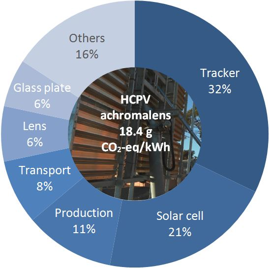
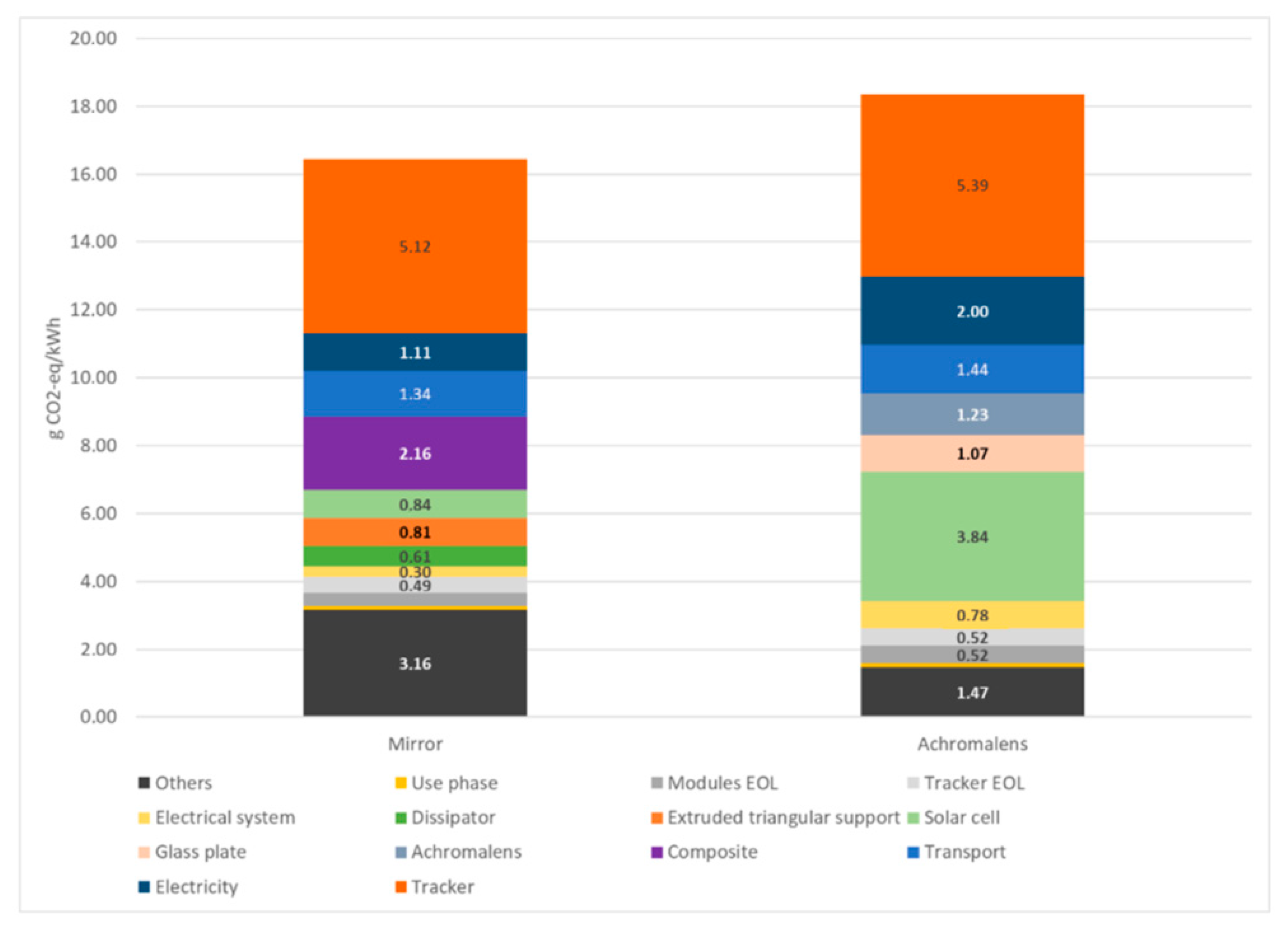
We determine the electricity generation of the tracking system based in Catania where the Direct Normal Irradiation (DNI) with a two-axis tracker is 2400 kWh/m2/year. The irradiation (I) for a two-axis tracker is 3040 kWh/m2/year (Global Normal Irradiance, GNI) taken from the PVGIS website [56].
The evaluation of a variety of losses of the modules is assessed in accordance with the literature [30,31]. This origin of the losses yields to: Converter losses (5%), dust deposition (2%), shading (1.5%), mismatch (2%), wiring losses (2%), availability (3%), light-induced degradation (1.5%), glass absorption (2%), and losses of limit on elevation angle (1%). Therefore, the ideal generation of one unit of CPV module is lowered by 20%.
The generation of electricity (E) can be expressed in Equation (2).
E = n = 1 30 I * A * η mod * η system * ( 1 d ) n 1
where I is the irradiation, A is the total module area, ηmod is the module efficiency, ηsystem is the system efficiency (80%), and d is the annual degradation (0.7%).
In accordance with Equations (1) and (2), the mirror and the two lens systems’ electricity amount exported to the grid over 30 years is respectively 1.71 and 1.62 GWh. For each impact category, the total impact of the system is divided by the electricity production in order to calculate the impact per kWh.

6.2. Climate Change

Impact assessment on climate is based on IPCC 2007 characterization factors. Figure 2 presents the climate change process impact distribution for both the mirror and the achromatic lens systems. The electricity considered represents the consumption during the module’s manufacturing phase. In addition, the electrical system is modeled including the DC-DC converter, electrical cables, and both the inverter and the transformer needed for the two-axis tracker. The “Others” category gathers all material inputs with a specific contribution included in the production and the assembly of the CPV modules. As presented in Figure 2, the results are expressed in g CO2-eq/kWh. Hence, we divided the total climate change impact by the total electricity exported to the grid (Eexport).
Following the LCA rules indicated in the ILCD handbook, the greenhouse gas emissions of the three CPV systems are evaluated as an equivalent of CO2, over a time horizon of 100 years.
The climate change impact ranges from 16.4 g CO2-eq/kWh for mirror modules to 18.4 g CO2-eq/kWh for Achromalens modules. The Fresnel lens system is lowered by 8% compared to the achromatic lens system due to the smaller impact of Fresnel lenses. Mirror modules are about 10% lower than Achromalens ones. Considering the early stage of the design of the technologies, this result of 10% of difference looks rather small and does not allow us to ensure that one technology will be better than the other one in the end. Nevertheless, the disaggregation of the results at process level allows us to identify the most impactful processes. Tracking and concentrating equipment is the main contributor to this category. Significant GHG emissions are related to the tracker (31%) and composite (13%) for the mirror scenario.
Due to a higher cell concentration per module area unit, the four-junction cell contribution is significant (21%). Electricity consumption for assembling the components of the module (11%) and Achromalens (7%) are also responsible for the damage.
Carbon dioxide (>90%) and methane (about 6%) emissions in the air are the most significant impact in this category for all scenarios.

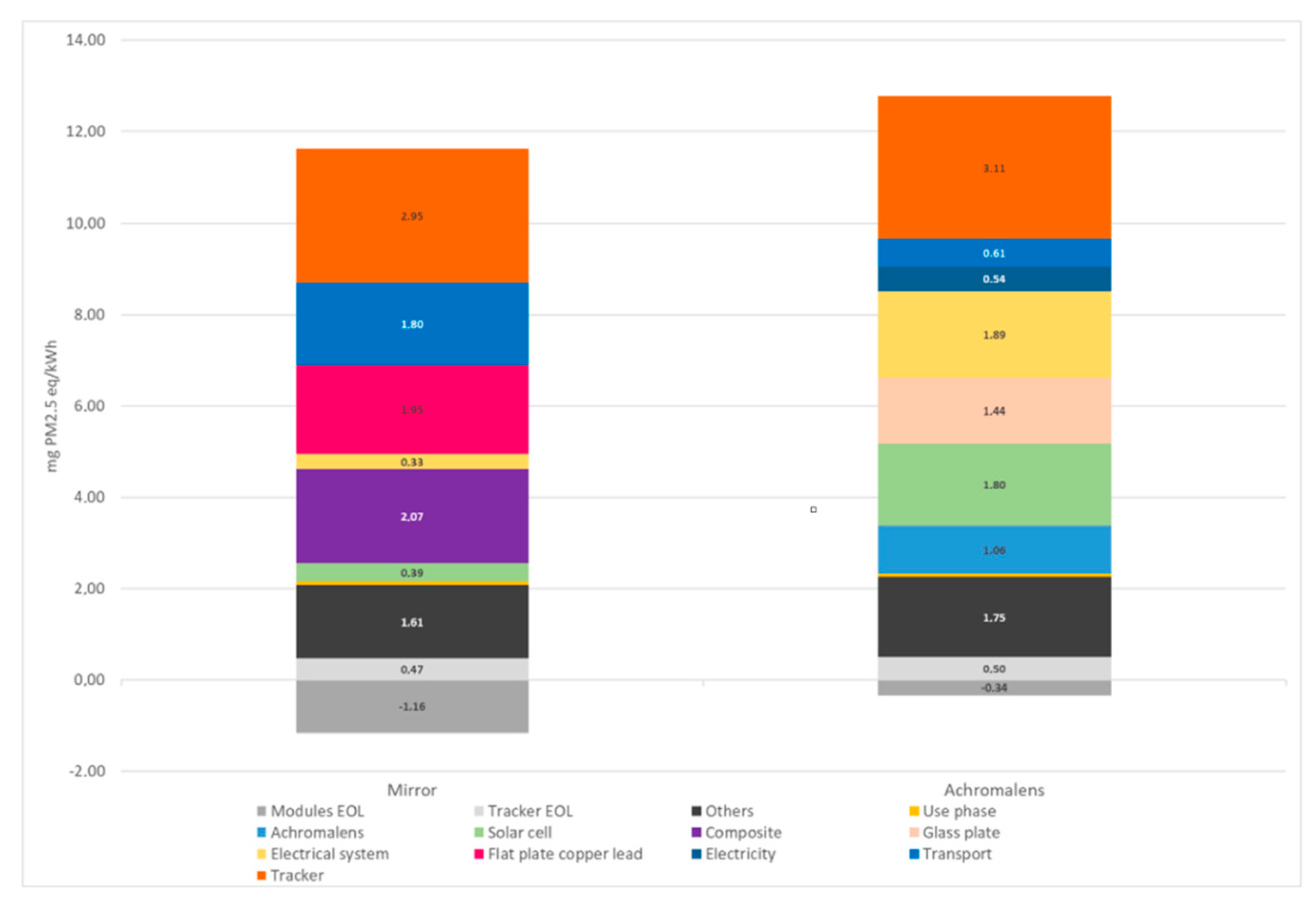
6.3. Particulate Matter
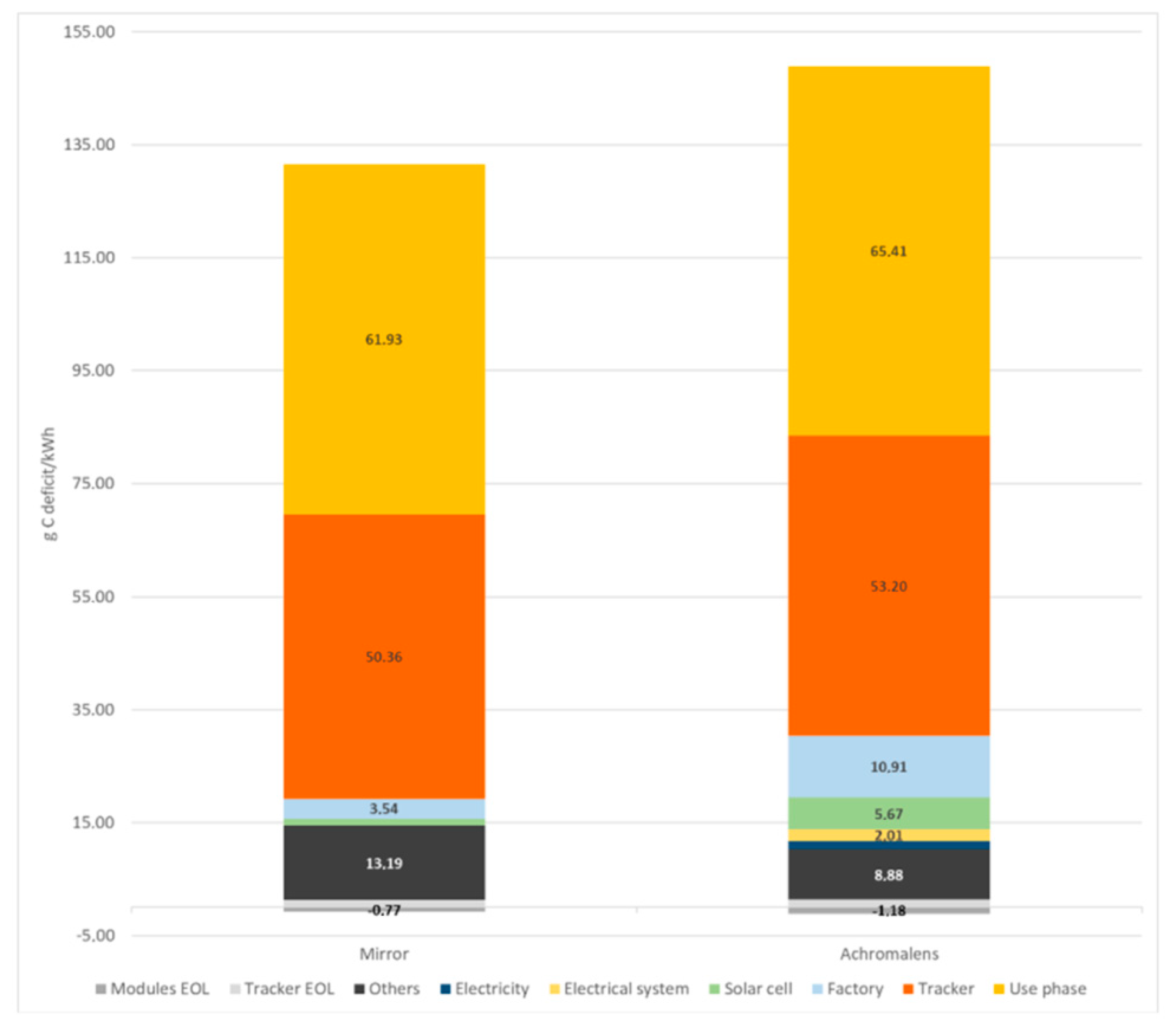
The impact due to the emissions of particulate matter is calculated using the Rabl and Spadaro model [51]. Figure 3 presents impacts from particles with detailed contribution per process.
The emissions of 11.8 mg PM2.5-eq/kWh for the mirror scenario is attributable to processes belonging to the extraction and materials phases. Tracker (25%), composite (17%), and copper (16%) are the most important contributors. Concerning the achromatic lens system, contributions come mainly from the tracker (25%), electrical systems (15%), solar cells (14%), and the glass plate (12%). The smaller surface of lens modules per tracker explains the small difference with the mirror scenario (67.20 versus 70.99 m2).
Moreover, heavier mirror modules explain the different impact of transportation with the two lens systems. The higher cell number per unit area for lens systems due to a lower concentration factor is responsible for the higher contribution of this sub-system. The greater impact of the achromatic lens compared to the Fresnel lens system (+7.5%) is due to the important amount of polycarbonate in achromatic lenses. Composite material (polycarbonate with glass fiber used for mirror support) can have a significant contribution.
The benefits of recycling metals such as copper, gold, and silver are important in the end-of-life phase, which has a positive contribution (negative impact) on this category for the three scenarios.
Particulates with a diameter less than 2.5 µm (>60%) and sulfur dioxide (about 30%) are the most emitted emissions in this category for every scenario.

6.4. Land Use

Land use is modeled using the characterization models of Mila I Canals [52] with characterization factors published by ILCD 2011, as presented in Figure 4.
We assess land use in the life cycle of the three HCPV scenarios. Both the achromatic and the Fresnel lens scenarios have a more significant potential impact compared to the mirror scenario. The results of the two lens systems are quite similar (+1% for the achromatic system due to the presence of polycarbonate in the lens).
The greater impact of the factory for the lens system is explained by the identical volume production assumption. Moreover, the less important electricity amount exported to the grid by the two lens systems due to a lower aperture area explains the higher ‘land use impact’ of the use phase and the tracker.
Occupation of grassland is the most impactful elementary flow in this category for all scenarios.

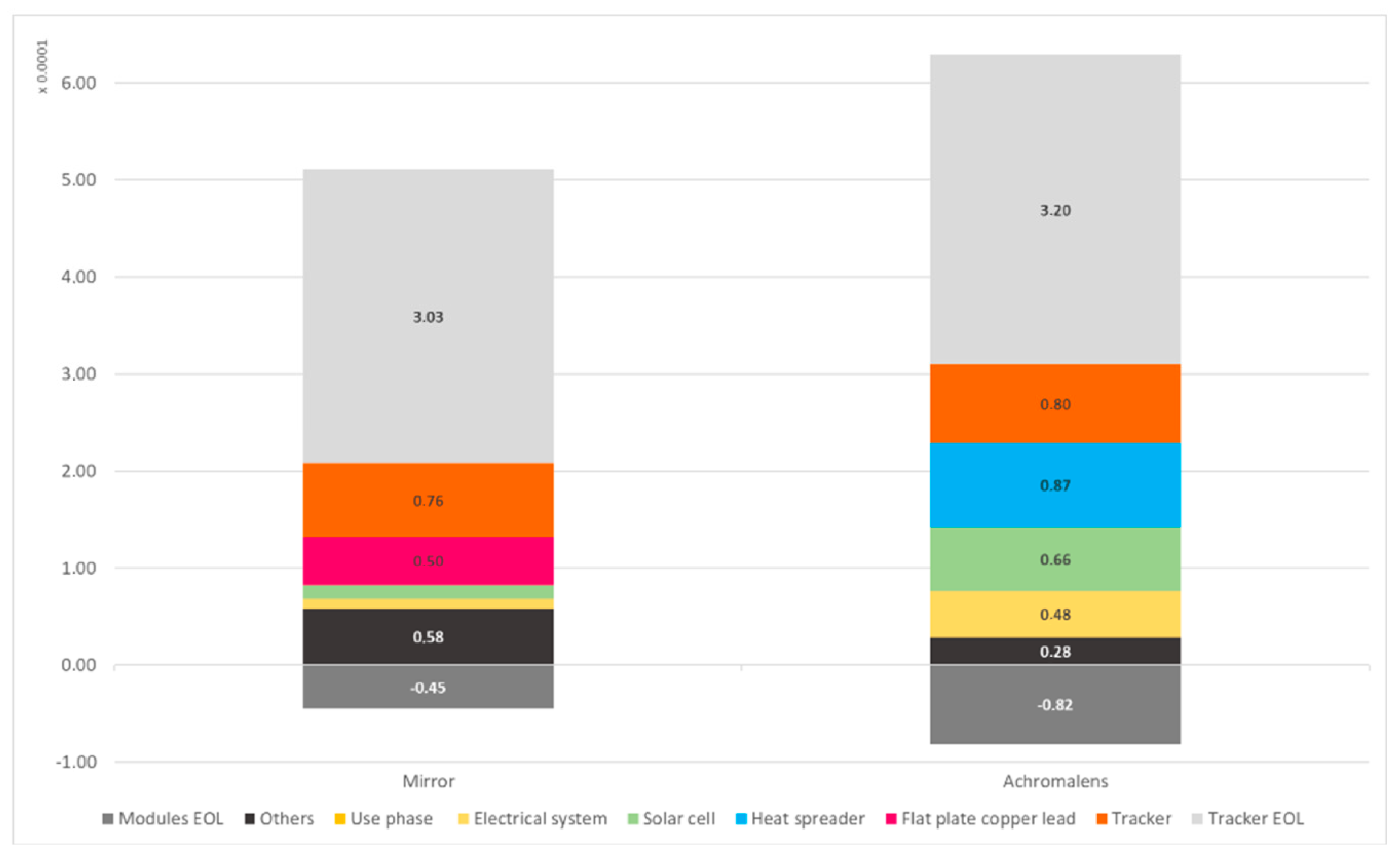
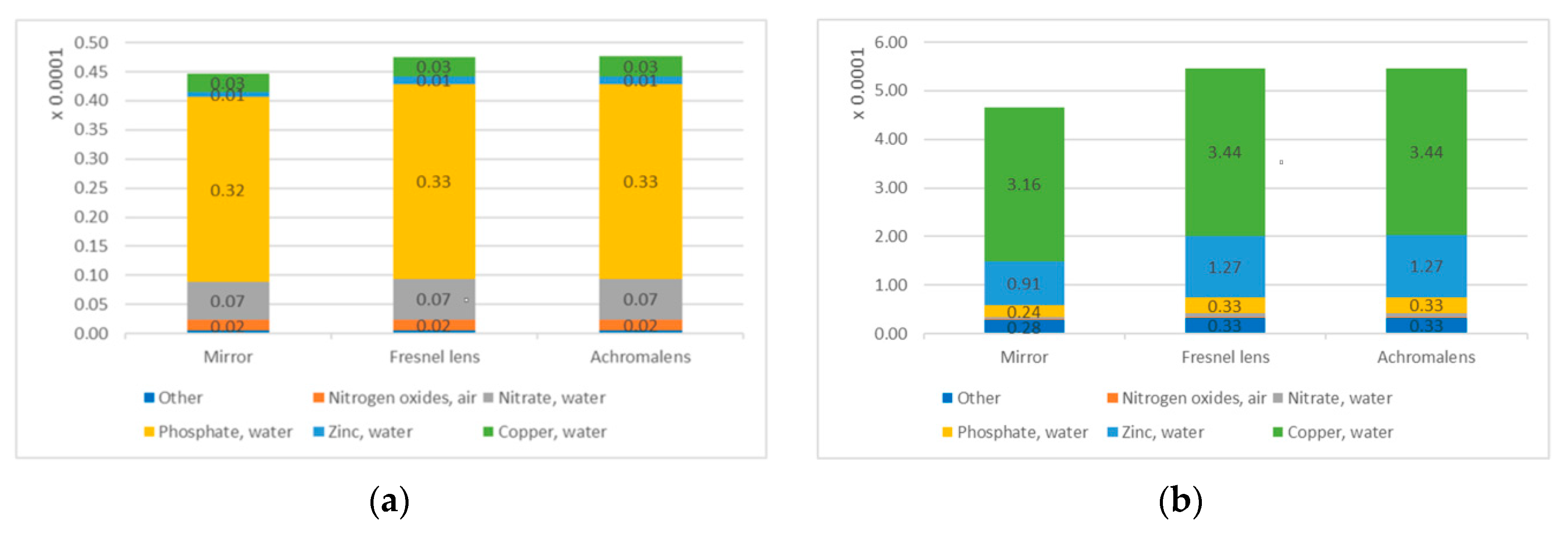
6.5. Aquatic Biodiversity

We assessed the impact of the three HCPV modules on aquatic biodiversity through three impact categories. Freshwater ecotoxicity, and marine and freshwater eutrophication impact results are normalized and weighted. The weighted impact (WIIC) is calculated as follows:
WI IC =   IP IC * WF IC NF IC          
where WIIC is the weighted impact, IPIC is the impact potential, NFIC and WFIC are, respectively, the normalization and weighting factors for an impact category [43].
The weighted impact from Freshwater ecotoxicity, and marine and freshwater eutrophication are presented in Figure 5 and can also be called weighted results.
Both achromatic and Fresnel lens HCPV systems’ impact on biodiversity are more important than that of the mirror one. After weighting, freshwater ecotoxicity is the greatest contributor to the total impact (>90%). The higher amount of metals and the higher number of solar cells (gold and electricity consumption) are highly responsible for this difference.
Copper (65%) and zinc (22% on average) emissions in water are the most impactful elementary flows. Copper in water mainly comes from copper waste ending as scrap. Zinc emissions in water yield to gold extraction and production processes.

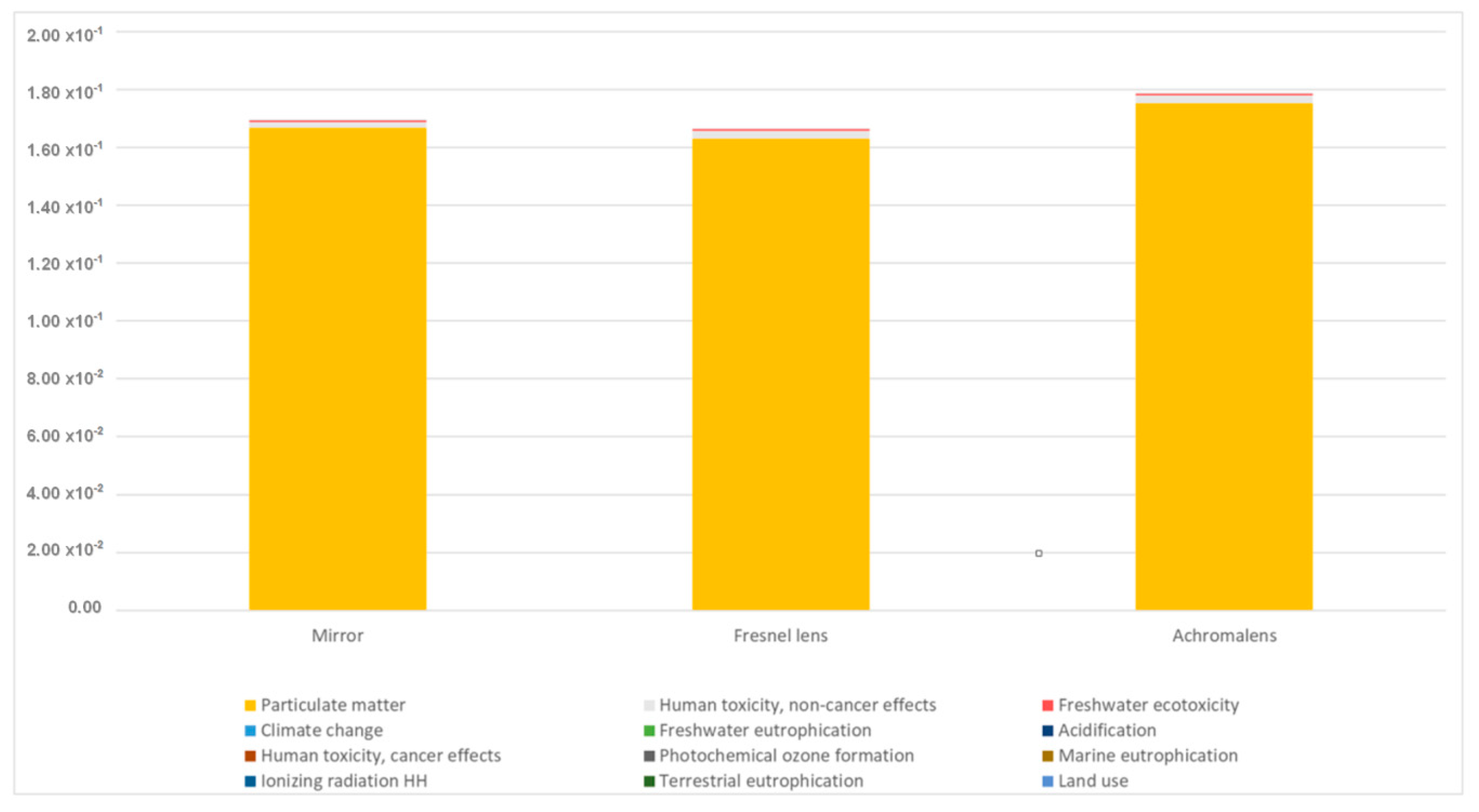
6.6. Single Score Results

The single score results are obtained with normalization and weighting factors from the PEFCR guidance [43] with toxicity categories. The single score result (S) for a HCPV system is obtained with the following equation:
S = n = 1 16 WI IC , n          
where S is the single score result and WIIC,n is the weighted impact (Equation (3)) of impact category n.
Figure 6 presents the single score results (without mineral, fossil, or renewable depletion weighted impact potential). The normalized and weighted results do not include the mineral, fossil, or renewable resource depletion. Indeed, this impact is driving all the results with only one substance: Germanium from land. Existing studies show that this is likely due to outdated and missing characterization factors [57,58,59].
The Achromalens system’s weighted results are more important than those of the mirror ones. Particulate matter is the most impacted category on Figure 6. The Fresnel lens impacts are higher than the mirror system’s impacts, except for the particulate matter category. Nevertheless, the difference between the two systems for this category is significant enough to explain the higher weighted results of the mirror system compared to the Fresnel lens system.
PM2.5 and sulfur dioxide emissions in the air are by far the most impacting elementary flows in the environment.

7. Discussion

We investigated three HCPV modules mounted with III-V four-junction cells (FJCs) during the CPVMatch research project. In this study, the role of concentration factors, glass coating, FJCs, and module efficiency are especially studied. The discussions below reflect the interpretation of the LCA study and cover the three perspectives.

7.1. Discussing How Key Environmental Parameters Affect the Results

How does a change in cells and module efficiency affect the overall performance of the system?
The assumptions and the possible improvements of the design of the modules is the first perspective. It especially relates to the influence of the life duration of the modules and their efficiency, the choice of materials, the end-of-life and recycling phases, and the influence of the electricity mix of the production phase. The efficiency of high performance modules and four-junction cells reached 36.7% for the mirror module and 41.4% for the full glass Achromalens module. These results are promising and represent the top performance of the modules, and their lifetime is expected to be 30 years. We have a direct relationship between the performance of the modules and these two aspects. An increase of 5% of the efficiency of the module will reduce the impacts by 4%. While cell efficiency is still the focus, the module as a whole shall be considered.
How is the overall impact of the system is affected by an extended life span?
At the same time, an increase in the life duration allows the reduction of all impacts associated with the production and the end-of-life phases. These life cycle stages dominate all impact categories (with the exception of the land use impact category). A sensitivity analysis on the parameter indicates that when the system’s lifespan increases from 30 to 50 years, the damages reduce by 25% for nearly all impact categories. When the two-axis tracker life service is doubled, the damages reduce between 10% and 20% depending on the impact category.
How do module materials affect environmental impacts?
The choice of material also affects the impact of the system; the first priority is indeed to reduce the weight of the module with adequate materials and technologies. Nevertheless, as we can see in the results, the polycarbonate damage for climate change and particulate matter presented in the mirror module scenario is important. Other lightweight materials can reduce the impact [60].
Can modules’ end-of-life be optimized?
Another key aspect is the end-of-life phase of the modules. Thanks to the efforts made to concentrate the rays of the sun, only a small surface of active material is needed, using smaller quantities of potential contaminants such as indium or germanium. At the same time, the system has less components with a lower level of integration and thus is more prone to dismantling. Optimization of waste recycling requires optimizing three parameters: Reduce contamination, facilitate waste collection, and allow efficient dismantling. The technologies explored for the HCPV modules present promising perspectives for these three parameters which highly encourage recycling. Nevertheless, the amount of aluminum used in the production is high, and it is therefore important to foster the use of recycled aluminum. We consider that the recycling rate of aluminum for the modules is nearly 95% at its end-of-life. We therefore assume that aluminum is based on a rate of 5% virgin material and 95% recycled material. An alternative scenario with a 50% recycling rate only is tested during a sensitivity analysis. This increases the climate change impact by 27% for the mirror system and 4% for the two others scenarios.
How does the location of the installation influence the overall impact of the system?
The last key parameter identified is the location of the production of the modules. Indeed, the climate change category can be highly influenced by the manufacturing location of both the modules and the solar cells. Current calculations are performed based on a 2016 EU electricity mix. Nevertheless, a production located in a country with low carbon electricity (such as Sweden, Norway, or France) can decrease the carbon footprint by 20 to 35%. However, if a country with a high carbon footprint produces the module, the climate change impact can raise by 30 to 50%.

7.2. Important Aspect and Sensitivity Analysis Related to Impact Assessment Models

Applying a sensitivity analysis of impact assessment on aquatic biodiversity.
The modeling of the impacts is also important in the interpretation of the results. Special attention needs to be paid to the way aquatic biodiversity is calculated. Impact categories affecting aquatic biodiversity are less mature than other categories such as climate change. Nevertheless, such an evaluation is needed in the interpretation as it is an important concern for society. Several sensitivity analyses are performed for interpreting the results. The questions addressed with these analyses are detailed here after:
Do damage modeling methods present different results? Indeed, since weighted results do not necessarily reflect damage, a comparative sensitivity analysis is conducted with two different damage life cycle impact assessment (LCIA) methods: RECIPE [10] and IMPACT 2002+ [61]. Even if the impact values may change (since the units can be different), the impact ranking and ratios between scenarios present the same pattern as weighted results. The aquatic biodiversity evaluation is consistent with the results from existing life cycle impact assessment methods [10,61].
Do we have a bias in the assessment due to an impact overestimation of metals? Metals such as copper and zinc are the most impacting substances in this category. The USEtox method should be considered carefully. Complexation and speciation mechanisms are not taken into account in this LCA method [7,8,9]. Existing studies underline an important overestimation of metals’ characterization factors [62,63,64]. Following the suggestions from these publications, we recalculated the ecotoxicity impact on freshwater, dividing by 100 the characterization factors of metals emitted in water, air, and soil. This leads to a different ranking of impact categories’ contribution. While freshwater ecotoxicity is driving the impact in the first case, eutrophication in freshwater becomes the most important contributor in this sensitivity analysis. Switching from ILCD Midpoint+ to a reduced impact of metals, Freshwater ecotoxicity’s contribution changes from 93% to 12%, freshwater eutrophication from 6% to 70%, and marine eutrophication from 2% to 19%.
Figure 7 presents these results, comparing two ways of addressing impacts on aquatic biodiversity. Figure 7a presents the results of the calculation based on normalized and weighed impacts, following ILCD midpoint and PEF guidance indications. Figure 7b presents the results based on damage modeling.
Exploring the optimization of land use with CPV.
Impact on land use needs additional attention. The occupation of arable land (by the plant) plays an important role on the use phase [65]. Thanks to its high efficiency, a combination of both agriculture and concentrating photovoltaics can be explored [66,67]. This may reduce the competition between food production and solar electricity.
Relevance of resource depletion impact category.
Impact assessment on mineral resources depletion allows limited interpretation for the time being. Only one material (germanium) is driving 99% of the impacts and the CML method (used for resource modeling) lacks some key characterization factors and has not been updated for many years. Before going more in depth with this impact category, the method needs to be updated and its coherence with the critical materials list [68] explored. Normalization and weighting allowing the presentation of the results in a single score is always disputable. This is an optional step of the ISO standard of LCA, no consensus exists on this issue and the results strongly depend on background assumptions (location for normalization and method for weighting). Nevertheless, single scores are very consistent with all impact categories. The mirror system’s normalized and weighted results present three times less impacts than the two lens prototypes.

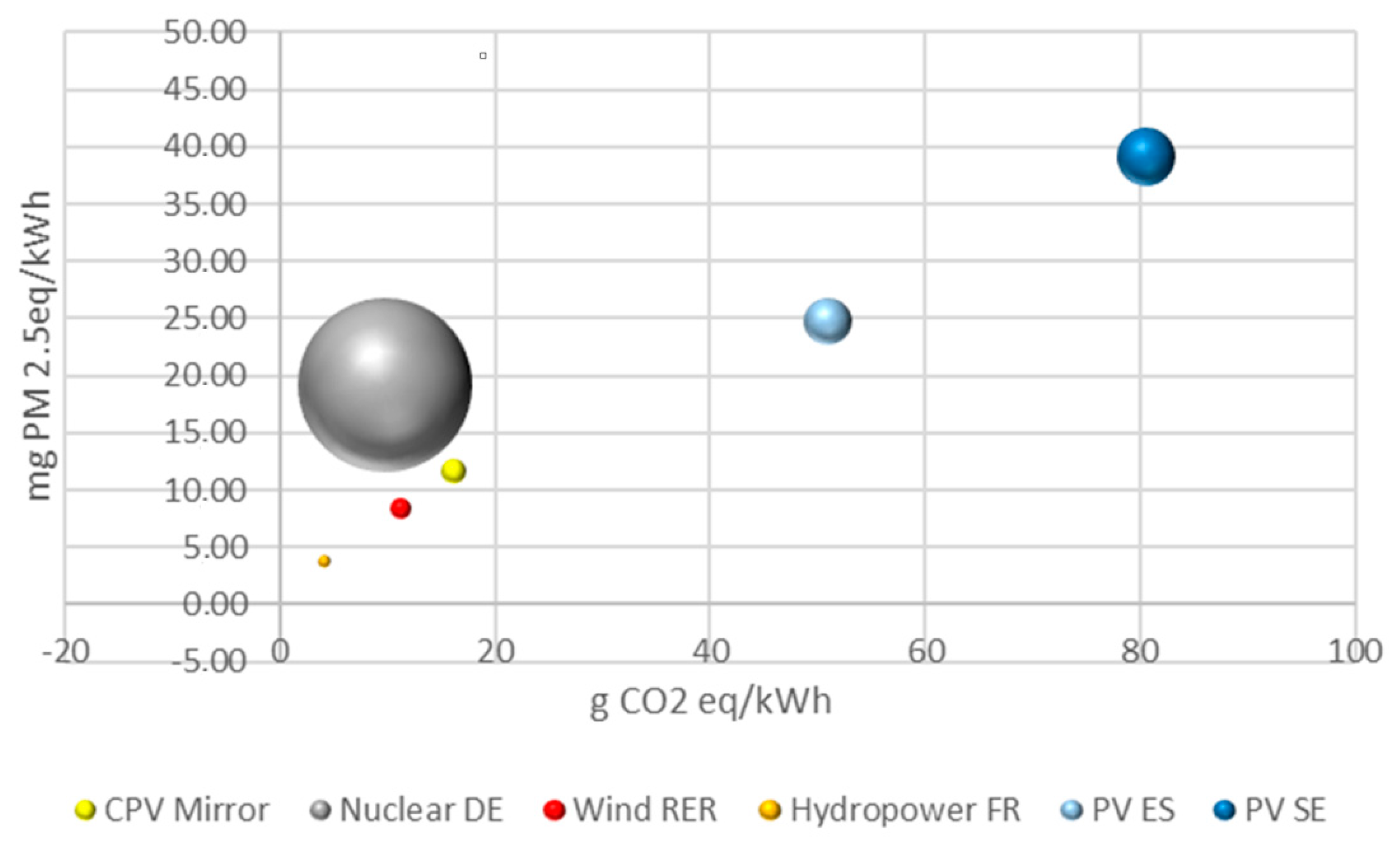
7.3. Comparing Environmental Performances of HCPV with Other Energy Sources

Beyond discussions on module design and impact assessment, HCPV technology ought to be compared with other electricity sources like fossil fuels and low-carbon-footprint electricity sources.
First, we compare HCPV’s performance with the most widely used fossil resources and then with the current renewable energy sources. Table 3 presents the environmental performance of HCPV mirrors compared to oil and coal electricity production in different countries.
The environmental impact of electricity from HCPV systems is in-between 50 and 100 times lower than fossil fuels for all impact categories. The climate change impact of fossil fuels ranges from 970 g to 1410 g CO2-eq/kWh (see Table 3). The difference between fossil fuels is due to the ratio of H/C which is higher for oil than for coal. Coal quality also influences carbon dioxide emissions. Concerning particles, current electricity production from coal in China features a significant difference compared to other sources. This is due to the power plant technology. Land use presents surprising results: Its impact is higher for fossil resources, especially for oil. This is due to land occupation of pipelines. In terms of non-renewable energy demand per kWh, all fossil resources present similar patterns, with on average 50 times more impact than HCPV.
A comparison is also conducted with low carbon energy sources. Figure 8 presents the positioning of six low carbon electricity means as for three parameters like carbon footprint, small particle emissions, and non-renewable primary energy demand.
HCPV performances are promising. Both in terms of carbon footprint and particle emissions, HCPV modules are in the low part of the curve with respectively less than 20 g CO2-eq/kWh, about 12 mg PM2.5-eq/kWh and 0.2 MJprim./kWh. This is just above very efficient renewable energy means, such as wind power and hydropower. Results are far lower than BIPV installed in Spain and Sweden, modeled with EcoInvent assumptions. Results can be smaller with open ground PV plants. The comparison between HCPV and nuclear power presents a similar range of results for greenhouse gas emissions (16 g and 10 g of CO2-eq/kWh, respectively) and particle emissions (12 and 19 PM2.5-eq/kWh, respectively). Nevertheless, compared to nuclear power, results for non-renewable primary energy demand is 50 times lower for HCPV. As what was done for fossil fuels, we also compared the performances of HCPV with other electricity sources for land use. The comparison with hydropower and nuclear power is, respectively, 4.2 and 19.9 g C deficit/kWh. This is respectively 30 times and six times lower than the CPV mirror. The comparison between HCPV and wind power presents very similar impacts on land use with, respectively, 131.3 and 132.2 C deficit/kWh.

7.4. Exploring the Possible Interest of HCPV Modules in a Circular Economy Perspective

Important environmental issues are now addressed with the emergence of the circular economy concept. There is not yet a world consensual definition of circular economy but the ADEME (French EPA) defines it as follows: “Circular economy can be defined as an economical system which aims at enhancing resources’ use efficiency, reducing environmental burdens, and improving human welfare for each parts of the life cycle of product and services” [71]. Based on this definition, it is interesting to investigate to which extent a novel technology or innovative product can meet circular economy’s expectations. Considering the HCPV technologies addressed in this article, several aspects can be further explored. In terms of efficient use of resources, thanks to the sun concentration and the high efficiency of cells, a reduced amount of material could be used per kWh produced. In terms of reduction of environmental burdens, the small surface of easily separable cells can support a more efficient material sorting at the end-of-life. This can allow higher recycling rates with lower contamination of recycled material. Recycling rates could therefore reach 90 to 95% based on existing recycling technologies with lower level of contamination of recycling material. As an example, current recycling of silicon PV only allows 80% of recycling rate (only glass and part of metals), and is impeded by a high level of contamination of EVA and silicon residues.

8. Conclusions

This article presents the main results of the environmental performances of HCPV innovative technologies. Beyond the improvement of the technological performances of HCPV, thanks to module efficiency, sun concentration and four-junction cells’ environmental performance is demonstrated in this article, which details the potential environmental impacts of three HCPV module prototypes. The results underline the potential of CPV toward the energy transition. In terms of climate change, results indicate that emissions per kWh of such systems can range from 16.4 to 18.4 g CO2-eq/kWh. This is close to wind energy (around 13 g CO2/kWh in the EcoInvent database). While this work enables the optimization of the cell and the modules, the results point out that the tracker should also be optimized. Exploring a possible downsizing of the trackers with lighter modules is also promising.
Another area of optimization is electricity consumption for producing the cells and the modules. Producing these systems in areas with low carbon electricity would strongly augment the environmental performances of HCPV modules.
Even assuming an average European electricity mix, the Energy Payback Time (EPBT) of the three systems ranges from 0.74 to 0.98 years and the Carbon Payback Time (CPBT) ranges from 0.98 to 1.1 years. However, the study is not limited to energy and carbon, and the 16 impact categories of the ILCD handbook are presented in Appendix B.
HCPV’s environmental performances are comprehensively examined and compared with the environmental burdens of electricity originating from oil and coal. As for the four impact categories considered, the environmental performances are improved on average by a factor ranging from 50 to 100. When the comparison is extended to renewable energy sources and nuclear power, the results show that HCPV lies within the range of low carbon emissions technologies, a little bit higher than wind power, hydropower, and nuclear power. Still, the difference in terms of primary energy needs per produced kWh highlights the performances of HCPV compared to nuclear power (about 50 times lower).
Also in terms of circular economy, as discussed above, HCPV technology requires a low surface of active material and a lower level of integration compared to other PV technologies. This is promising from a circular economy perspective, since it requires less semi-conductor materials during production and opens the way to a dismantling and a lower contamination by toxic substances during the end-of-life phase. Yet, since HCPV technology was not originally designed from a circular economy perspective, it necessitates further research works and improvements to fully demonstrate better performances. Nevertheless, as mentioned below, a higher efficiency and lower integration of components bring about promising perspectives such as lower environmental burdens, increased recyclability, and improved reparability.
Beyond these promising aspects, several points require further investigation. The resource’s impact category cannot be interpreted, although it is a crucial issue in terms of circular economy perspective. The current method available for modeling resource depletion [69] in LCA is outdated and does not cover all the materials used for producing PV semi-conductors and electronic components [59]; neither does it address the issue of critical materials [58,68]. It is, indeed, also crucial to look at this impact category, even if it requires research efforts so as to ensure the coherence between criticality and mineral depletion. The impact of fine particles shall also be explored more in depth. Indeed, particle emission reduction seems obvious from fossil fuels to HCPV, but the current impact of particles at global level is considerable (around 8% of deaths in the world) [2], so two important points should be investigated: First, life cycle inventory (LCI) data reliability (ensuring that particle emission reduction can occur during the production phase of the modules); secondly, estimation of the external cost of particles emissions on health (in order to better reflect the benefits of HCPV modules). We can also bear in mind that all renewable energy technologies are quickly changing over time. HCPV cost is likely to decrease with time; optimizing HCPV’s environmental performance and simultaneously reducing the costs is likely to pave the way for innovative solutions. HCPV technology is currently limited to the sunbelt area, but further cost reduction may foster installations in other areas, opening the market to new technologies with a small environmental footprint.

Supplementary Materials

Detailed Life Cycle Inventories used in this study are available online as unit processes at https://www.mdpi.com/1996-1073/12/15/2916/s1 supplementary materials_Life cycle assessment of new high concentration photovoltaic modules (HCPV) and multi-junction cells-Detailed Life Cycle Inventories analysis.

Author Contributions

J.P. and T.G. have together contributed to perform the study and elaborate this article.

Funding

This life cycle assessment study was conducted within the European Union’s Horizon 2020 Research and Innovation Programme under grant agreement No. 640873.

Conflicts of Interest

The authors declare no conflicts of interest.

Glossary

Alloc DefAllocation default
BIPVBuilding Integrated Photovoltaics
EPBTEnergy Payback Time
EVAEthylene vinyl acetate
CHSwitzerland
CNChina
CPBTCarbon Payback Time
CPVConcentrated photovoltaics
EOLEnd-Of-Life
FJCsFour-junction cells
GeGermanium
GLOWorld
HCPVHigh concentrated photovoltaics
IEAInternational Energy Agency
ILCDInternational Reference for Life Cycle Data system
kWhKilo-Watt per hour
kWpKilo-Watt peak
LCALife Cycle Assessment
LCILife Cycle Inventory
LCIALife Cycle impact Assessment
MAMorocco
MJprimMegajoule primary
PEFProduct Environmental Footprint
REREurope
RoWRest of World
UUnit process
USUnited States of America

Appendix A

Table A1. World electricity modeling with EcoInvent data [70] in accordance with International Energy Agency [1] information.
EcoInvent 3.3 Process20072016
Electricity, hard coal, at power plant/CN U41.2%38.3%
Electricity, oil, at power plant/FR U5.5%3.7%
Electricity, natural gas, at power plant/US U21.2%23.1%
Electricity, low voltage {CH}| treatment of biogas, burned in micro gas turbine 100 kWe | Alloc Def, U1.0%1.8%
Electricity, production mix photovoltaic, at plant/CH U0.01%1.3%
Electricity, at wind power plant 800 kW/RER U0.9%3.8%
Electricity from waste, at municipal waste incineration plant/CH U0.3%0.4%
Electricity, nuclear, at power plant/CH U13.7%10.4%
Electricity, hydropower, at power plant/FR U15.9%16.7%
Electricity, high voltage {RoW}| electricity production, geothermal | Alloc Def, U0.3%0.3%
Table A2. World primary energy supply modeling with EcoInvent data [70] in accordance with IEA [1] information.
EcoInvent 3.3 Process200720122016
Hard coal, burned in power plant/CN U27.5%29.0%27.1%
Heavy fuel oil, burned in power plant/FR U33.7%31.7%31.9%
Natural gas, burned in power plant/US U20.8%21.4%22.1%
Electricity, low voltage {CH}| treatment of biogas, burned in micro gas turbine 100 kWe | Alloc Def, U9.4%9.5%9.8%
Electricity, nuclear, at power plant/CH U5.8%4.8%4.9%
Electricity, hydropower, at power plant/FR U2.2%2.4%2.5%
Electricity, high voltage {RoW}| electricity production, geothermal | Alloc Def, U0.7%1.1%1.6%
Table A3. 2012 World final consumption modeling with EcoInvent data [70] in accordance with IEA [1] information.
EcoInvent 3.3 ProcessRepartition
Hard coal, burned in power plant/CN U12.1%
Heavy fuel oil, burned in power plant/FR U39.8%
Natural gas, burned in power plant/US U15.1%
Electricity, low voltage {CH}| treatment of biogas, burned in micro gas turbine 100 kWe | Alloc Def, U11.3%
Electricity, production mix photovoltaic, at plant/CH U0.3%
Other processes
Electricity17.9%
Heat3.2%

Appendix B

Table A4. Impact assessment results (per kWh).
CategoryUnitMirrorFresnel LensAchromalens
Climate changeg CO2-eq16.417.118.4
Ozone depletionµg CFC-11-eq1.692.012.06
Human toxicity, non-cancer effectsCTUh3.59 × 10−84.85 × 10−84.87 × 10−8
Human toxicity, cancer effectsCTUh2.46 × 10−92.88 × 10−92.92 × 10−9
Particulate mattermg PM2.5-eq11.911.612.5
Ionizing radiation HHBq U235-eq3.515.055.13
Ionizing radiation E (interim)CTUe8.49 × 10−91.10 × 10−81.12 × 10−8
Photochemical ozone formationmg NMVOC-eq55.062.165.0
Acidificationmmolc H+-eq1.16 × 10−11.31 × 10−11.36 × 10−1
Terrestrial eutrophicationmmolc N-eq1.90 × 10−12.22 × 10−12.31 × 10−1
Freshwater eutrophicationmg P-eq22.130.430.5
Marine eutrophicationmg N-eq57.586.388.0
Freshwater ecotoxicityCTUe2.683.103.11
Land useg C deficit1.31 × 1021.46 × 1021.47 × 102
Water resource depletionmL wate-eq44.81.05 × 1021.06 × 102
Mineral, fossil & ren resource depletiong Sb-eq3.5716.316.3
Table A5. Life cycle expectancies of HCPV system components.
ComponentLife Cycle Span (Years)
Two-axis tracker30
HCPV module30
Cables30
Manufacturing plant30
Inverter15
Transformer10

References

  1. IEA. IEA Website. Available online: https://www.iea.org/statistics/ (accessed on 10 March 2019).
  2. Landrigan, P.J.; Fuller, R.; Acosta, N.J.R.; Adeyi, O.; Arnold, R.; Basu, N.N.; Baldé, A.B.; Bertollini, R.; Bose-O’Reilly, S.; Boufford, J.I.; et al. The Lancet Commission on pollution and health. Lancet 2018, 391, 462–512. [Google Scholar] [CrossRef] [Green Version]
  3. MacKay, D.J.C. Solar energy in the context of energy use, energy transportation and energy storage. Philos. Trans. R. Soc. A Math. Phys. Eng. Sci. 2013, 371. [Google Scholar] [CrossRef] [PubMed]
  4. Capellán-Pérez, I.; de Castro, C.; Arto, I. Assessing vulnerabilities and limits in the transition to renewable energies: Land requirements under 100% solar energy scenarios. Renew. Sustain. Energy Rev. 2017, 77, 760–782. [Google Scholar] [CrossRef] [Green Version]
  5. Broswimmer, F.; Écocide, L. Une brève histoire de l’extinction en masse des espèces; Paragon: Paris, France, 2003. [Google Scholar]
  6. Novacek, M. Terra: Our 100-Million-Year-Old Ecosystem--and the Threats That Now Put It at Risk; Farrar, Straus and Giroux: New York, NY, USA, 2008. [Google Scholar]
  7. Rosenbaum, R.K.; Bachmann, T.M.; Gold, L.S.; Huijbregts, M.A.J.; Jolliet, O.; Juraske, R.; Koehler, A.; Larsen, H.F.; MacLeod, M.; Margni, M.; et al. USEtox - The UNEP-SETAC toxicity model: Recommended characterisation factors for human toxicity and freshwater ecotoxicity in life cycle impact assessment. Int. J. Life Cycle Assess. 2008, 13, 532–546. [Google Scholar] [CrossRef]
  8. Henderson, A.D.; Hauschild, M.Z.; Van De Meent, D.; Huijbregts, M.A.J.; Larsen, H.F.; Margni, M.; McKone, T.E.; Payet, J.; Rosenbaum, R.K.; Jolliet, O. USEtox fate and ecotoxicity factors for comparative assessment of toxic emissions in life cycle analysis: Sensitivity to key chemical properties. Int. J. Life Cycle Assess. 2011, 16, 701–709. [Google Scholar] [CrossRef]
  9. Pennington, D.W.; Payet, J.; Hauschild, M. Aquatic ecotoxicological indicators in life-cycle assessment. Environ. Toxicol. Chem. 2004, 23, 1796–1807. [Google Scholar] [CrossRef]
  10. Struijs, J.; Beusen, A.; van Jaarsveld, H.; Huijbregts, M.A.J. Aquatic Eutrophication. Chapter 6. In ReCiPe 2008—A Life Cycle Impact Assessment Method Which Comprises Harmonised Category Indicators at the Midpoint and the Endpoint Level, 1st ed.; Report I: Characterisation Factors; Goedkoop, M., Heijungs, R., Huijbregts, M.A.J., De Schryver, A., Struijs, J., Van Zelm, R., Eds.; VROM: Barendrecht, The Netherlands, 2009. [Google Scholar]
  11. Seppälä, J.; Posch, M.; Johansson, M.; Hettelingh, J.P. Country-dependent characterisation factors for acidification and terrestrial eutrophication based on accumulated exceedance as an impact category indicator. Int. J. Life Cycle Assess. 2006, 11, 403–416. [Google Scholar] [CrossRef]
  12. Posch, M.; Seppälä, J.; Hettelingh, J.P.; Johansson, M.; Margni, M.; Jolliet, O. The role of atmospheric dispersion models and ecosystem sensitivity in the determination of characterisation factors for acidifying and eutrophying emissions in LCIA. Int. J. Life Cycle Assess. 2008, 13, 477–486. [Google Scholar] [CrossRef]
  13. Payet, J. Assessing toxic impacts on aquatic ecosystems in LCA. Int. J. Life Cycle Assess. 2005, 10, 373. [Google Scholar] [CrossRef]
  14. Pang, M.; Zhang, L.; Wang, C.; Liu, G. Environmental life cycle assessment of a small hydropower plant in China. Int. J. Life Cycle Assess. 2015, 20, 796–806. [Google Scholar] [CrossRef]
  15. Flury, K.; Frischknecht, R. Life Cycle Inventories of Hydroelectric Power Generation; ESU-services Ltd.: Kanzleistrasse, Switzerland, 2012. [Google Scholar]
  16. Guezuraga, B.; Zauner, R.; Pölz, W. Life cycle assessment of two different 2 MW class wind turbines. Renew. Energy 2012, 37, 37–44. [Google Scholar] [CrossRef]
  17. Crago, C.L.; Koegler, E. Drivers of growth in commercial-scale solar PV capacity. Energy Policy 2018, 120, 481–491. [Google Scholar] [CrossRef]
  18. Masson, G.; Orlandi, S.; Rekinger, M. Global Market Outlook for Photovoltaics 2013-2017; Solar Power Europe: Brussels, Belgium, 2013. [Google Scholar]
  19. Uwe, F.; Göran, B.; Annette, C.; Francis, J.; Virginia, D.; Hans, L.; Navin, S.; Helen, W.; Jeremy, W. Energy and Land Use—Global Land Outlook Working Paper; UNCCD: Bonn, Germany, 2017. [Google Scholar] [CrossRef]
  20. Hernandez, R.R.; Hoffacker, M.K.; Murphy-Mariscal, M.L.; Wu, G.C.; Allen, M.F. Solar energy development impacts on land cover change and protected areas. Proc. Natl. Acad. Sci. USA 2015, 112, 13579–13584. [Google Scholar] [CrossRef] [PubMed] [Green Version]
  21. Hoffacker, M.K.; Allen, M.F.; Hernandez, R.R. Land-Sparing Opportunities for Solar Energy Development in Agricultural Landscapes: A Case Study of the Great Central Valley, CA, United States. Environ. Sci. Technol. 2017, 51, 14472–14482. [Google Scholar] [CrossRef] [PubMed] [Green Version]
  22. Piemonte, V.; De Falco, M.; Tarquini, P.; Giaconia, A. Life Cycle Assessment of a high temperature molten salt concentrated solar power plant. Sol. Energy 2011, 85, 1101–1108. [Google Scholar] [CrossRef]
  23. Renno, C. Experimental and theoretical analysis of a linear focus CPV/T system for cogeneration purposes. Energies 2018, 11, 2960. [Google Scholar] [CrossRef]
  24. Gomaa, M.R.; Mustafa, R.J.; Rezk, H.; Al-Dhaifallah, M.; Al-Salaymeh, A. Sizing methodology of a multi-mirror solar concentrated hybrid PV/thermal system. Energies 2018, 11, 3276. [Google Scholar] [CrossRef]
  25. Vallerotto, G.; Victoria, M.; Askins, S.; Antón, I.; Sala, G. Improvements in the manufacturing process of achromatic doublet on glass (ADG) Fresnel lens. In AIP Conference Proceedings; AIP Publishing: Melville, NY, USA, 2018. [Google Scholar] [CrossRef]
  26. Vallerotto, G.; Victoria, M.; Askins, S.; Herrero, R.; Domínguez, C.; Antón, I.; Sala, G. Design and modeling of a cost-effective achromatic Fresnel lens for concentrating photovoltaics. Opt. Express 2016, 24, A1245. [Google Scholar] [CrossRef] [PubMed]
  27. Dimroth, F.; Tibbits, T.N.D.; Niemeyer, M.; Predan, F.; Beutel, P.; Karcher, C.; Oliva, E.; Siefer, G.; Lackner, D.; Fuß-kailuweit, P.; et al. Four-Junction Wafer-Bonded Concentrator Solar Cells. IEEE J. Photovolt. 2015, 6, 343–349. [Google Scholar] [CrossRef]
  28. Corona, B.; Escudero, L.; Quéméré, G.; Luque-Heredia, I.; San Miguel, G. Energy and environmental life cycle assessment of a high concentration photovoltaic power plant in Morocco. Int. J. Life Cycle Assess. 2017, 22, 364–373. [Google Scholar] [CrossRef]
  29. RSE. Results of the APOLLON Project and Concentrating Photovoltaic Perspective; Ricerca sul Sistema Energetico—RSE S.p.A.: Milan, Italy, 2014. [Google Scholar]
  30. Scholten, M.D.W.; Cassagne, V.; Huld, T. Solar Resources and Carbon Footprint of Photovoltaic Power in Different Regions in Europe. In Proceedings of the 29th European PV Solar Energy Conference, Amsterdam, The Netherlands, 22–26 September 2014; pp. 3421–3430. [Google Scholar]
  31. Fthenakis, V.M.; Kim, H.C. Life cycle assessment of high-concentration photovoltaic systems. Prog. Photovolt. Res. Appl. 2009, 17, 11–33. [Google Scholar] [CrossRef]
  32. Kim, H.C.; Fthenakis, V.M. Life cycle energy demand and greenhouse gas emissions from an amonix high concentrator photovoltaic system. In Proceedings of the 2006 IEEE 4th World Conference on Photovoltaic Energy Conference, Waikoloa, HI, USA, 7–12 May 2006; pp. 628–631. [Google Scholar]
  33. Matzer, R.; Peharz, G.; Patyk, A.; Dimroth, F.; Bett, A.W. Life cycle assessment of the concentrating photovoltaic system FLATCON. In Advances in Energy Studies 2008: Towards an Holistic Approach Based on Science and Humanity; Workshop: Graz, Austria, 2008. [Google Scholar]
  34. Agustín-Sáenz, C.; Sánchez-García, J.Á.; Machado, M.; Brizuela, M.; Zubillaga, O.; Tercjak, A. Broadband antireflective coating stack based on mesoporous silica by acid-catalyzed sol-gel method for concentrated photovoltaic application. Sol. Energy Mater. Sol. Cells 2018, 186, 154–164. [Google Scholar] [CrossRef]
  35. Alonso, R.; Pereda, A.; Bilbao, E.; Cortajarena, J.A.; Vidaurrazaga, I.; Román, E. Design and analysis of performance of a DC power optimizer for HCPV systems within CPVMatch project. AIP Conf. Proc. 2018, 2012, 050001. [Google Scholar]
  36. Van Riesen, S.; Neubauer, M.; Boos, A.; Rico, M.M.; Gourdel, C.; Wanka, S.; Krause, R.; Guernard, P.; Gombert, A. New module design with 4-junction solar cells for high efficiencies. In Proceedings of the 11th International Conference on Concentrator Photovoltaic Systems (CPV-11), AIP Conference Proceedings 1679, Aix-les-Bains, France, 13–15 April 2015; p. 100006. [Google Scholar]
  37. European Commission Eurostat. Available online: http://ec.europa.eu/eurostat/statistics-explained/index.php/Electricity_production,_consumption_and_market_overview/fr (accessed on 10 February 2019).
  38. Payet, J.; Evon, B.; Sié, M.; Blanc, I.; Beloin-Saint-Pierre, D.; Adra, N.; Raison, E.; Puech, C.; Durand, Y. Référentiel d’évaluation des Impacts Environnementaux des Systèmes Photovoltaïques par la Méthode D’analyse du Cycle de Vie; Cycleco: Ambérieu-en-Bugey, France, 2011. [Google Scholar]
  39. Jolliet, O.; Soucy, G.; Houillon, G. Analyse du cycle de vie: comprendre et réaliser un écobilan, 3rd ed.; Presses Polytechniques et Universitaires Romandes: Lausanne, Switzerland, 2010; ISBN 2880748860. [Google Scholar]
  40. ISO 14040. Environmental Management—Life Cycle Assessment—Principles and Framework; ISO: Geneva, Switzerland, 2006. [Google Scholar]
  41. ISO 14044. Gestion environnementale—Analyse du Cycle de vie— Exigences et Lignes Directrices; ISO: Geneva, Switzerland, 2006. [Google Scholar]
  42. ILCD. European Commission—Joint Research Centre—Institute for Environment and Sustainability: International Reference Life Cycle Data System (ILCD) Handbook—General Guide for Life Cycle Assessment—Detailed Guidance, 1st ed.; EUR 24708 EN.; Publications Office of the European Union: Luxembourg, 2010. [Google Scholar]
  43. European Commission. PEFCR Guidance Document, Guidance for the 14 Development of Product Environmental Footprint Category Rules (PEFCRs); version 6.3; European Commission: Brussels, Belgium, 2017.
  44. De Haes, H.A.U.; Sleeswijk, A.W.; Heijungs, R. Similarities, differences and synergisms between HERA and LCA - An analysis at three levels. Hum. Ecol. Risk Assess. 2006, 12, 431–449. [Google Scholar] [CrossRef]
  45. Perpinan, O.; Lorenzo, E.; Castro, M.A.; Eyras, R. Energy Payback Time of Grid Connected PV Systems: Comparison Between Tracking and Fixed Systems. Prog. Photovolt. Res. Appl. 2009, 17, 137–147. [Google Scholar] [CrossRef]
  46. Alsema, E.A.; Wild-Scholten, M.J.d. Environmental impact of crystalline silicon photovoltaic module production. In Proceedings of the CIRP International Conference on Life Cycle Engineering, Leuven, Belgium, 31 May–2 June 2006. [Google Scholar]
  47. Constantino, G.; Freitas, M.; Fidelis, N.; Pereira, M.G. Adoption of photovoltaic systems along a sure path: A life-cycle assessment (LCA) study applied to the analysis of GHG emission impacts. Energies 2018, 11, 2806. [Google Scholar] [CrossRef]
  48. Nishimura, A.; Hayashi, Y.; Tanaka, K.; Hirota, M.; Kato, S.; Ito, M.; Araki, K.; Hu, E.J. Life cycle assessment and evaluation of energy payback time on high-concentration photovoltaic power generation system. Appl. Energy 2010, 87, 2797–2807. [Google Scholar] [CrossRef]
  49. Kommalapati, R.; Kadiyala, A.; Shahriar, M.T.; Huque, Z. Review of the life cycle greenhouse gas emissions from different photovoltaic and concentrating solar power electricity generation systems. Energies 2017, 10, 350. [Google Scholar] [CrossRef]
  50. Edenhofer, O.; Pichs-Madruga, R.; Sokona, Y.; Farahani, E.; Kadner, S.; Seyboth, K.; Adler, A.; Baum, I.; Brunner, S.; Eickemeier, P.; et al. (Eds.) Climate Change 2014: Mitigation of Climate Change; Contribution of Working Group III to the Fifth Assessment Report of the Intergovernmental Panel on Climate Change; Cambridge University Press: Cambridge, UK; New York, NY, USA, 2014. [Google Scholar]
  51. Rabl, A.; Spadaro, J.V. The RiskPoll Software, Version is 1.051. 2004. Available online: http://www.arirabl.com (accessed on 1 August 2004).
  52. Milà i Canals, L.; Romanyà, J.; Cowell, S.J. Method for assessing impacts on life support functions (LSF) related to the use of “fertile land” in Life Cycle Assessment (LCA). J. Clean. Prod. 2007, 15, 1426–1440. [Google Scholar] [CrossRef]
  53. Staudinger, J.; Keoleian, G.A.; Flynn, M.S. Management of End-of Life Vehicles (ELVs) in the US; University of Michigan: Washtenaw, MI, USA, 2001. [Google Scholar]
  54. Latunussa, C.E.L.; Ardente, F.; Blengini, G.A.; Mancini, L. Life Cycle Assessment of an innovative recycling process for crystalline silicon photovoltaic panels. Sol. Energy Mater. Sol. Cells 2016, 156, 101–111. [Google Scholar] [CrossRef]
  55. Rathod, K.; Gupta, S.; Sharma, A.; Prakash, S. Energy-Efficient Melting Technologies in Foundry Industry. Indian Foundry J. 2016, 62, 39–46. [Google Scholar]
  56. Šúri, M.; Huld, T.A.; Dunlop, E.D. PV-GIS: A web-based solar radiation database for the calculation of PV potential in Europe. Int. J. Sustain. Energy 2005, 24, 55–67. [Google Scholar] [CrossRef]
  57. Adibi, N.; Lafhaj, Z.; Gemechu, E.D.; Sonnemann, G.; Payet, J. Introducing a multi-criteria indicator to better evaluate impacts of rare earth materials production and consumption in life cycle assessment. J. Rare Earths 2014, 32, 288–292. [Google Scholar] [CrossRef]
  58. Adibi, N.; Lafhaj, Z.; Yehya, M.; Payet, J. Global Resource Indicator for life cycle impact assessment: Applied in wind turbine case study. J. Clean. Prod. 2017, 165, 1517–1528. [Google Scholar] [CrossRef]
  59. Adibi, N.; Lafhaj, Z.; Payet, J. New resource assessment characterization factors for rare earth elements: applied in NdFeB permanent magnet case study. Int. J. Life Cycle Assess. 2019, 24, 712–724. [Google Scholar] [CrossRef]
  60. Witik, R.A.; Payet, J.; Michaud, V.; Ludwig, C.; Månson, J.A.E. Assessing the life cycle costs and environmental performance of lightweight materials in automobile applications. Compos. Part A Appl. Sci. Manuf. 2011, 42, 1694–1709. [Google Scholar] [CrossRef]
  61. Jolliet, O.; Margni, M.; Charles, R.; Humbert, S.; Payet, J.; Rebitzer, G. IMPACT 2002+: A New Life Cycle Impact Assessment Methodology. Ind. Ecol. 2003, 8, 324–330. [Google Scholar] [CrossRef]
  62. Dong, Y.; Gandhi, N.; Hauschild, M.Z. Development of Comparative Toxicity Potentials of 14 cationic metals in freshwater. Chemosphere 2014, 112, 26–33. [Google Scholar] [CrossRef] [PubMed]
  63. Dong, Y.; Rosenbaum, R.K.; Hauschild, M.Z. Assessment of Metal Toxicity in Marine Ecosystems: Comparative Toxicity Potentials for Nine Cationic Metals in Coastal Seawater. Environ. Sci. Technol. 2016, 50, 269–278. [Google Scholar] [CrossRef] [PubMed]
  64. Haye, S.; Slaveykova, V.I.; Payet, J. Terrestrial ecotoxicity and effect factors of metals in life cycle assessment (LCA). Chemosphere 2007, 68, 1489–1496. [Google Scholar] [CrossRef] [PubMed]
  65. Zhang, Z.; Zhang, F.; Li, M.; Liu, L.; Liu, W.; Lv, H.; Liu, Y.; Yao, P.; Liu, W.; Ou, Q.; et al. Progress in agriculture photovoltaic leveraging CPV. AIP Conf. Proc. 2018, 2012, 110006. [Google Scholar]
  66. Hyder, F.; Baredar, P.; Sudhakar, K.; Mamat, R. Performance and land footprint analysis of a solar photovoltaic tree. J. Clean. Prod. 2018, 187, 432–448. [Google Scholar] [CrossRef]
  67. Poggi, F.; Firmino, A.; Amado, M. Planning renewable energy in rural areas: Impacts on occupation and land use. Energy 2018, 155, 630–640. [Google Scholar] [CrossRef]
  68. Mathieux, F.; Ardente, F.; Bobba, S.; Nuss, P.; Blengini, G.; Alves Dias, P.; Blagoeva, D.; Torres De Matos, C.; Wittmer, D.; Pavel, C.; et al. Critical Raw Materials and the Circular Economy—Background Report; JRC Science-for-Policy Report, EUR 28832 EN; Publications Office of the European Union: Luxembourg, 2017; ISBN 978-92-79-74282-8. [Google Scholar] [CrossRef]
  69. Van Oers, L.; de Koning, A.; Guinee, J.B.; Huppes, G. Abiotic Resource Depletion in LCA; Road and Hydraulic Engineering Institute, Ministry of Transport and Water: Amsterdam, The Netherlands, 2002. [Google Scholar]
  70. Wernet, G.; Bauer, C.; Steubing, B.; Reinhard, J.; Moreno-Ruiz, E.; Weidema, B. The ecoinvent database version 3 (part I): overview and methodology. Int. J. Life Cycle Assess. 2016, 21, 1218–1230. [Google Scholar] [CrossRef]
  71. Geldron, A. Economie Circulaire: Notions; ADEME: Vonges, France, 2014; pp. 1–9. [Google Scholar]
Figure 1. Life cycle of the High Concentration Photovoltaic (HCPV) system. It is a cradle-to-grave approach. Solar cells, HCPV modules, electronic components, and the two-axis tracker manufacturing are taken into account. Transportation is included between extraction and manufacturing, installation, use, dismantling, and end-of-life. A factory is considered for the manufacturing of four-junction cells (FJCs), receivers, and modules. However, only energy inputs (diesel, electricity) are included for dismantling and component separation. The boundary between the system and the ecosphere is represented as the green dashed line, which thus represents the limits of the technosphere. The boundaries between background and foreground system is represented with the dark dashed line.
Energies 12 02916 g001
Figure 2. The results of impacts on climate change are expressed in g CO2-eq impact per process distribution. The sum of all processes for mirror and Achromalens systems corresponds to 16.4 and 18.4 g CO2-eq/kWh, respectively. All processes contributing to more than 5% are detailed. Smaller processes are gathered in “Others”.
Energies 12 02916 g002
Figure 3. Impact on human health due to small particle emissions. Most impacting are the mirror and Achromalens module components’ and life cycle stages’ contribution to particulate matter. All processes contributing to more than 5% are detailed. Less significant contributors are gathered in the “Others” category. The total impacts potential is 11.8 and 12.4 mg PM2.5-eq/kWh, respectively, for the mirror and the Achromalens systems. Environmental benefits due to system extension thanks to metal recycling are responsible for the negative impacts.
Energies 12 02916 g003
Figure 4. Land-use impact distribution for the mirror and the achromatic lens systems. The mirror system impact is 131.3 g C deficit. However, the achromatic system impact is 147.8 g C deficit. All processes contributing to more than 5% are detailed. Less significant processes are gathered in the “Others” category. Small benefits from recycling metals (gold in particular) explain the negative impact from the modules’ end-of-life.
Energies 12 02916 g004
Figure 5. The most impactful module components and life cycle stages to aquatic biodiversity weighted results. Mirror and Achromalens systems’ total results are, respectively, 4.67 × 10⁻⁴ and 5.48 × 10⁻⁴ pts. All processes contributing to more than 5% are detailed. Less significant processes are gathered in the “Others” category. Benefits from modules’ end-of-life (EOL) stage are due to the recycling of metals (copper, gold, and silver).
Energies 12 02916 g005
Figure 6. Weighted results excluding the mineral depletion category. Mirror, Fresnel lens, and Achromalens results are, respectively, 0.169, 0.166, and 0.179 pts. The particulate matter impact category domination represents 98%.
Energies 12 02916 g006
Figure 7. Normalized and weighted results of substances emitted in the environment for the three scenarios. (a) The left bars the results of the ILCD Midpoint+ method; (b) The right bars represent the results with metals freshwater ecotoxicity’s weighted results divided by 100. The results differ by a factor of 10. From left to right, the total results are 4.66 × 10⁻⁴, 5.46 × 10⁻⁴, and 5.47 × 10⁻⁴, and 4.46 × 10⁻⁵, 4.76 × 10⁻⁵, and 4.76 × 10⁻⁵ pts.
Energies 12 02916 g007
Figure 8. Environmental impact of low carbon energy sources. Energy demand (MJ) compared to particulate matter emissions (PM2.5-eq) and climate change (g CO2-eq). The size of the bubbles is proportional to their non-renewable primary energy demand, calculated using the CML methodology [69]. The two other impact categories stem from the ILCD Midpoint 2011 methodology. From left to right in the legend, energy demand is, respectively, 0.2, 11.6, 0.2, 0.05, 0.8, and 1.3 MJprim/kWh. HCPV results are compared with EcoInvent data for low carbon electricity sources.
Energies 12 02916 g008
Table 1. Set of parameters for the three HCPV prototypes.
Scenario MirrorFresnel LensAchromalens
Nominal powerWp361.86117.44117.44
Module efficiency%36.736.736.7
Concentration ratio 800320320
Aperture aream20.9860.320.32
Modules on trackerPc72210210
Table 2. End-of-life processes for materials and corresponding unit flows selected in ecoinvent.
MaterialsEnd-of-Life Process Names
Electronic components
DC-DC converter, printed wiring boards
Disposal, treatment of printed wiring boards/GLO U and Disposal, municipal solid waste, 22.9% water, to sanitary landfill/CH U
Glass
Glass plate, solar glass
Disposal, glass, 0% water, to inert material landfill/CH U
Metals recycled part
Copper, gold, silver
Electricity, medium voltage, RER (0.65 kWh/kg)
with output material [name of metal], {GLO}| market for | Alloc Def, U
Others
Silicone product, glass fiber, copper waste, diode, cadmium, butyl acrylate, bisphenol A powder, tetrachlorosilane, epoxy resin
Disposal, municipal solid waste, 22.9% water, to sanitary landfill/CH U
Plastics
Polycarbonate, Nylon 6-6, vinyl acetate
Disposal, plastics, mixture, 15.3% water, to municipal incineration/CH Uand Steam, in chemical industry {GLO}| market for | Alloc Def, U
Solar cellHazardous waste, for underground deposit {GLO}| market for | Alloc Def, U
SteelSteel and iron (waste treatment) {GLO}| recycling of steel and iron | Alloc Def, Uand Steel, low-alloyed {GLO}| market for | Alloc Def, U (output to technosphere)
Table 3. Environmental impact assessment results for 1 kWh stemming from different energy sources. The first three categories are obtained with the ILCD Midpoint+ 2011 method and the last one with the Cumulative Energy Demand version 1.0.9 [69] method. ES, SE, PL, and CN represent, respectively, Spain, Sweden, Poland, and China. Impact of fossil resources are calculated using the EcoInvent database [70].
CategoryUnitHCPV MirrorOil ESCoal PLCoal CN
Climate changeg CO2-eq16.4970.91151.11409.9
Particulate mattermg PM2.5-eq11.8524.9405.53320.7
Land useg C deficit131.33017.2586.5773.4
Non-renewable primary energy demandMJ0.213.613.512.1

