Investigation on the Impact of Air Admission in a Prototype Francis Turbine at Low-Load Operation

Abstract

Due to significant changes in the energy system, hydraulic turbines are required to operate over a wide power range. In particular, older turbines which are not designed for these environments will suffer under off-design conditions. In order to evaluate whether or not such a turbine could fulfill the new requirements of the energy market, a study about the behavior of a prototype plant in low-load operation is presented. Therefore, prototype site measurements are performed to determine the most damaging operating point by means of acceleration sensors and pressure transducers. Moreover, unsteady computational fluid dynamics (CFD) simulations considering two-phase flow and two hybrid turbulence models are used to analyze the flow conditions inside the turbine. The resulting pressure pulsations are mapped onto the runner blade to obtain stress and further calculate damage factors. Accordingly, the stresses are compared to those obtained by the strain gauge measurement. Moreover, the influence of active flow control by means of air injection on plant behavior and runner lifetime is discussed as well.

1. Introduction

Currently, the energy system is undergoing a truly disruptive transformation. The integration of renewable energy sources, driven by the need to address climate change can lead to instability and reliability issues in the electrical grid. Therefore, hydro power plants are supplying grid stabilization services of significant importance. However to provide those services, hydraulic machines have to operate under off-design conditions and further deal with transient behavior and fast response times [1]. Regarding Francis turbines, this leads to the occurrence of flow phenomena such as draft tube and channel vortices as well as vortex shedding and cavitation [2,3]. Thereby, strong pressure pulsations interact with the runner and other parts of the machine unit [4]. Furthermore, if the harmonic excitation of the flow phenomena is equal or close to a natural frequency of the structure, resonance can lead to soaring amplitudes [5]. In the case of the draft tube vortex with an exciting frequency of f/$f_0$ = 0.2–0.3 refereed to the runner rotational frequency $f_0$, this can lead to problems of generator resonance as already shown by Rheingans [6] in 1940. Therefore, the unsteady flow cannot only influence the runner fatigue [7], but also damage bearings and other structural parts of the machine unit. Especially, in the case of older hydro power plants, which are not designed for those operating ranges, this can lead to unplanned machine shut downs and thus to increased downtimes due to safety risks. To minimize the cost of operation and prevent expensive failure events [8,9], one has to reduce those vortex-induced-vibrations (VIV), while also mitigating pressure pulsations. This can be done by influencing the flow behavior by means of design modifications of the draft tube. There are various approaches of this so called passive method like draft tube fins [10] and runner cone extensions [11]. Another possibility would be active flow control by means of air or water injection. In addition to the vortex disturbance this can also add damping effects and change the natural frequency as reported in [12]. However, it can also have some contrary effects and lead to stability problems as described by Muntean et al. [13]. Another downside of the air injection technique, is the negative effect on the global efficiency as the hydraulic power is decreased by using air with lower density than water as second medium. Therefore, the relative air content has to be capped at a very low ratio. Typically, this value does not exceed $2.5\%$ of the turbine discharge [14]. Moreover, to induce air, a pressure difference is required and therefore energy is consumed. According to a study published by March [15], the efficiency losses for different air injection locations range from $0.2\%$ to $4\%$. Due to different Froude numbers and a lack of 1:1 reproductions of the machine set, model tests are usually not sufficient to investigate dynamical behavior [12]. To ensure an improvement of the machine behavior and in the wider sense, decrease fatigue damage, detailed prototype site measurements are required. Within this field of research, knowledge has been developed over several years [14,16] including recent works [17,18]. However, most studies dealing with the effects of air admission are done by using test rigs and model machines. Experimental investigations on computational fluid dynamics (CFD) can play an essential role, especially by describing the flow field and highlighting vortex structures. In the case of prototype machines with reduced options of measurement points compared to model tests, and without the possibility of visualization, simulations can be a viable complement. Therefore, CFD studies of prototype machines have been of great interest in recent years [19]. However, only a few of them are considering two phase flow and air injection [20]. Furthermore, using the obtained pressure fields for a transient finite element method (FEM) to capture dynamical stress showed accurate results [21,22]. The main aim of this work is an investigation of the off-design region, highlighting dynamical stresses, vibrations and their impact on the fatigue life. Moreover, the possibility to reduce those damaging effects by means of air admission and a comparison with the original state will be shown.

2. Prototype Site Measurements

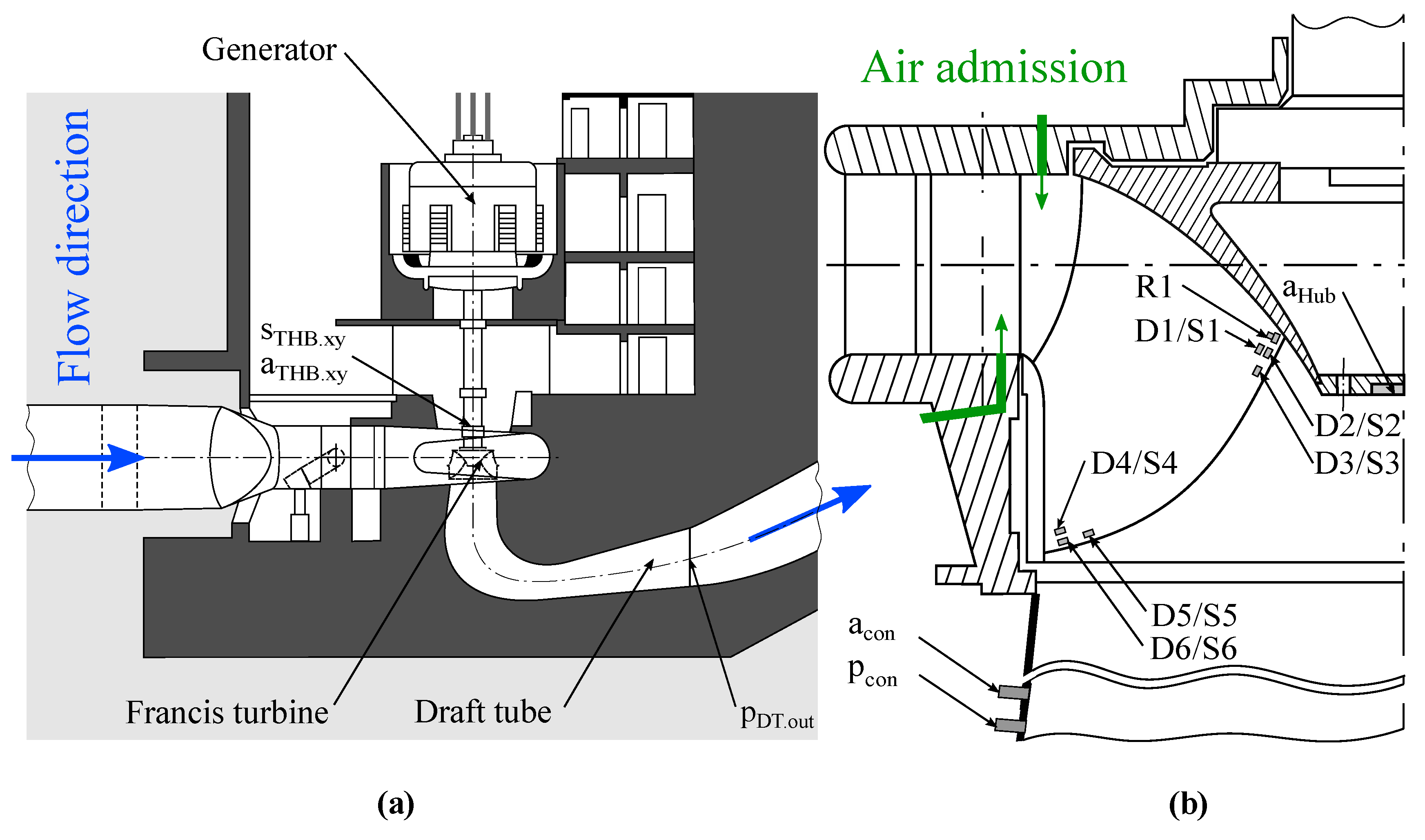
2.1. Prototype Unit and Experimental Setup

Within the course of a refurbishment project, prototype site measurements were performed on a hydro power plant equiped with two Francis turbine runners. The concerned Francis turbine can be considered as a medium head unit with a speed factor [23]

$$n_{ED}=n·\frac{D}{\sqrt{g·H}}\approx 0.39$$

(1)

using runner speed n and outer diameter D as well as gravity constant g and turbine head H. Additionally to the existing monitoring system, pressure transducers and vibration sensors as well as strain gauges were applied to investigate the behavior of the machine unit at off-design operation. Accordingly, Figure 1a,b is showing an overview of the power plant and sensor positions. Besides different uniaxial strain gauges on the runner blade suction side (S) and pressure side (D), Figure 1b also shows the position of the air admission. Additionally, a T-rosette (R1) is placed in the notch at the hub-side of the blade. Further details regarding the installation and the placement of the strain gauges can be seen in [24].

Wall pressure measurements are performed by the use of a fast response piezo-resistive transducer in a range of 0–10 bar with a maximum measurement uncertainty of $\pm 0.2\%$. The position of the sensor $p_{con}$ is illustrated in Figure 1b and the sampling rate is set to 3 kHz ensuring a sufficient range to capture pressure pulsations related to flow phenomena. The outlet pressure $p_{DT.out}$ is measured by a relative pressure transmitter in a range of 0–4 bar with a maximum measurement uncertainty of $\pm 0.2\%$ and a sampling rate of 100 Hz. Vibrations are measured at the positions according to Figure 1 with a sampling frequency of 3 kHz. There are several cases reported in the literature in which the effect of air on improving machine behavior in the low load range is investigated. Although most of them are suggesting to induce air directly in the draft tube [25,26] to disturb vortex formations, in this case the air injection is done upstream of the runner. Thereby, a higher pressure produced by the air compressor has to be used instead. However, this uncommon location should have the advantage of mitigate erosive action and reduce dynamical impact not only on the trailing edge, but on the entire runner [16].

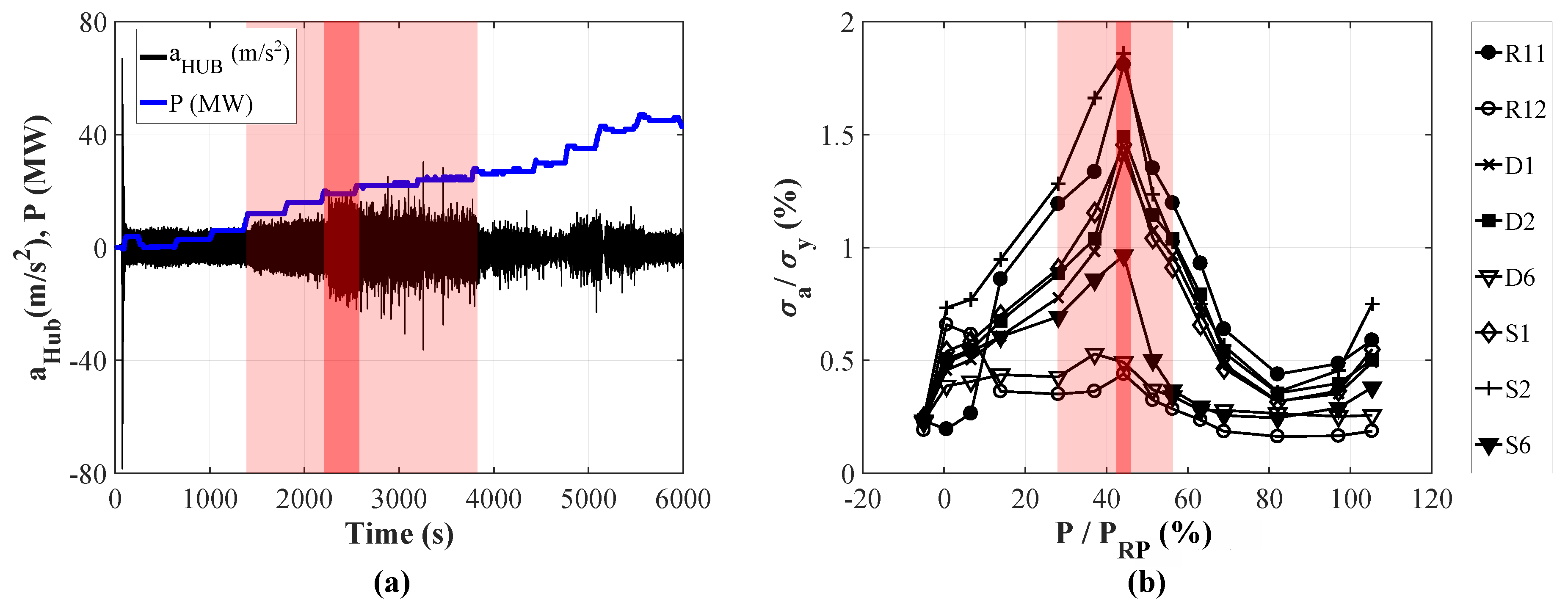
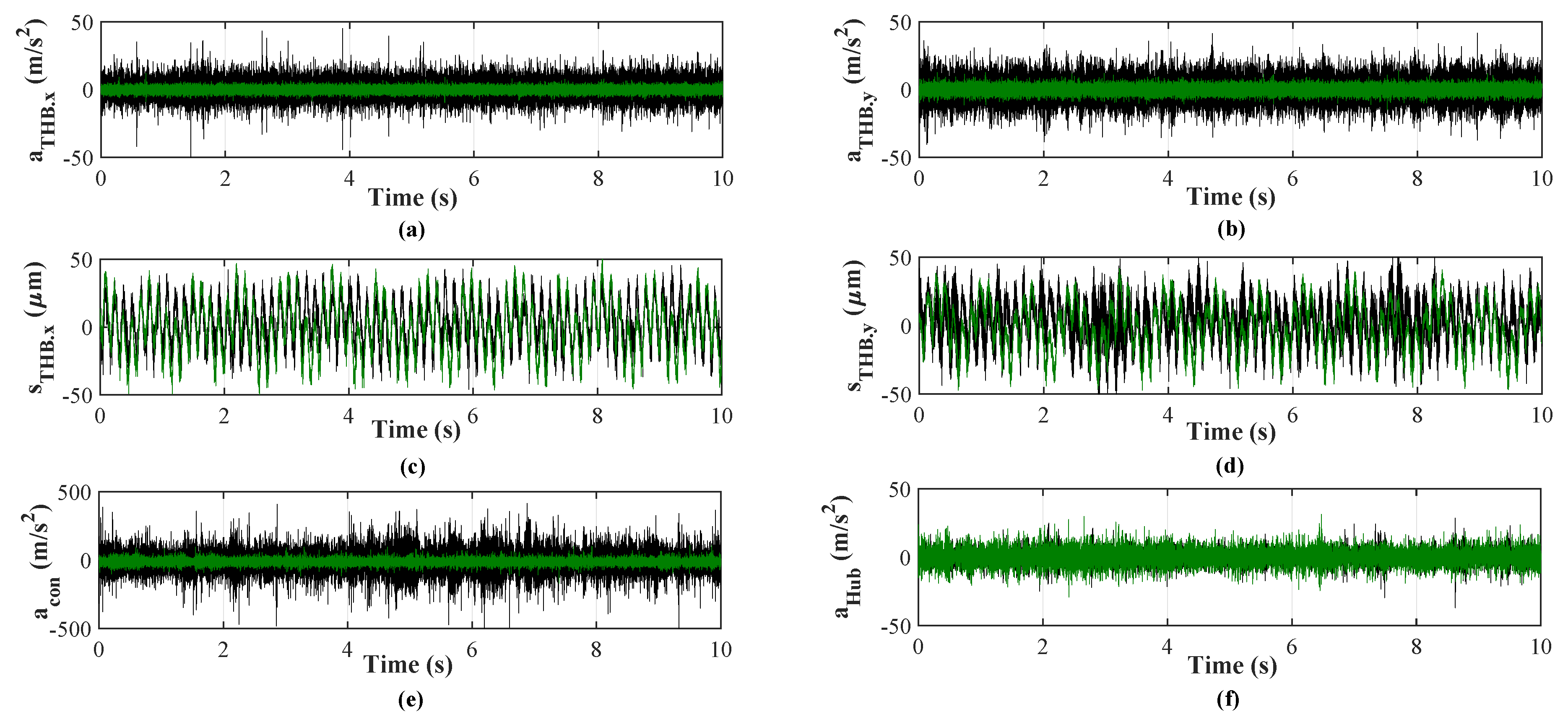
2.2. Measurement Procedure and Plant Behavior

The measurement procedure was defined based on the experience and observations of the plant operator and knowledge gained within the course of a previous research project. After the plant start-up Machine 1 was operating with stationary load points determined by constant guide vane opening and the power output (P), while Machine 2 was operating at the rated point (RP) to ensure constant conditions and omit influence of the secondary unit on the measurement as much as possible. According to Figure 2a, Machine 1 was operating at different load steps with a length of 5 or 10 min depending on the waterway oscillations and behavior of the machine set. After reaching full load, P was reduced again and the turbine was operated at several reference steps [24]. At approximately $63\%$ of the rated power $P_{RP}$ air was injected, with the aim to improve the machine behavior in low-load operation by suppressing pressure pulsations and consequently also vibrations.

Moreover, Figure 2a shows the signal of the acceleration sensor $a_{HUB}$ in time domain, while Figure 2b presents the results of the dynamical stress according to the strain gauge measurement published in [24]. Thereby, the amplitudes ${\sigma }_a$ are normalized with the yield strength ${\sigma }_y$ of the runner material. The red area represents the critical low-load region, especially highlighting the most critical operating point at $44\%·P_{RP}$. Comparing both signals to each other, one can see that high dynamical load corresponds to increased vibrations of the runner. Figure 3 shows the behavior of the machine set with (green) and without (black) air injection at the most critical load point. The effect in terms of damping and omitting vibrations can be seen at the turbine bearing by means of the acceleration sensors $a_{THB.x.y}$ in two planar directions. Accordingly, the sensor $a_{con}$ located at the draft tube wall, where the vibrations are significantly high without air admission, shows the same behavior. However all these sensors (Figure 3a,b,e are measuring the vibrations referred to the absolute system, which is in this case the powerhouse building. In contrast, the relative displacement transducers of the turbine bearing $s_{THB.x.y}$ (Figure 3c,d) showing a similar behavior with and without air injection. Moreover, the runner vibrations in z-direction $a_{HUB}$ (Figure 3f) are also not significantly impacted by air admission. Therefore, to determine the actual runner damage a fatigue analysis is required. Due to the use of a CFD simulation, possible excitation mechanism and corresponding frequencies of flow phenomena can be revealed.

3. Numerical Model

3.1. Geometry and Mesh

The 3D geometry model was prepared using available 2D drawings and test measurements. Moreover, the actual geometry of the runner blade was checked for deviations by the use of a 3D scanner. The turbine model consists of spiral casing (SC), stay vanes (SV), guide vanes (GV), runner (RN) and the draft tube (DT) (see Figure 4). Only a few simplifications are made to reduce the complexity of the model e.g., the fillet radius on the stay vanes and the labyrinth seals are not modeled. The majority of the hexahedral meshes is generated using the commercial software ANSYS ICEM (Version $18.1$, ANSYS, Canonsburg, PA, USA). The only exception is the runner, where NUMECA AUTOGRID5 (Version $12.2$, NUMECA, Brussels, Belgium) is used. More information about the meshing including a grid independence study according to Celik [27] is published in [21]. In addition to the standard RN model, a second finer mesh (RN VS) with refinements especially around the trailing edge is created. According to Figure 1, a number of 24 at the hub and shroud circumferential distributed air inlets are included in a slightly refined GV domain (GVA). The whole mesh consists of around 25 million cells including the RN domain and around 37 million cells, if the RN VS is used (see

Table 1. Mesh size and quality. In addition to the standard RN model, a second finer mesh (RN VS) with refinements especially around the trailing edge; a slightly refined GV domain (GVA).

Domain	SC	SV	GV	RN	DT	GVA	RN VS
Number of cells (million)	$1.7$	$1.3$	$3.2$	$8.8$	$10.5$	$3.7$	20
Minimum determinant (-)	$0.2$	$0.28$	$0.7$	$0.26$	$0.7$	$0.412$	$0.27$
Minimum angle (${}^{\circ }$)	$10.3$	$24.9$	$18.2$	$26.1$	27	$33.75$	$20.3$
$y_{mean}^{+}$ (-)	$27.3$	$16.4$	32	$12.4$	$11.1$	$25.4$	$11.6$

).

3.2. CFD-Setup

The commercial solver ANSYS CFX (Version $19.1$, ANSYS, Canonsburg, PA, USA) was used to approximate turbulence based on the Navier–Stokes equations. As it was mentioned by Eichhorn [22] amongst others, the application of scale-resolving simulation (SRS) hybrid turbulence models leads to a better prediction of the pressure pulsation inside the runner and draft tube. Therefore, the SAS (scale adaptive simulation) and the newer SBES (stress blended eddy simulation) are applied and compared to each other. The SAS model is an improved unsteady Reynolds-averaged Navier–Stokes (URANS) formulation based on the introduction of the von Karman length-scale to divide into regions with steady or unsteady flow. In steady regions the k–$\omega$–SST (shear stress transport) a Reynolds-averaged Navier–Stokes (RANS) model published by Menter [28] is used. To enable large eddy simulation (LES) behavior at unsteady flow regions an additional source term $Q_{SAS}$ depending on the quadratic length scale ratio is introduced by Egorov and Menter [29]. Contrary, the SBES model is a further development of the grid resolution depending detached eddy simulation (DES) models. One of the greatest weaknesses of the original DES formulation is the boundary layer treatment, due to the dependency on the grid resolution. Therefore, the SBES model as proposed by Menter et al. [30] focuses on the improvement of the shielding function to protect the RANS boundary layers. Although the detailed formulation of the switching function remains unpublished currently, the application of this rather new model provides some proven benefits. In contrast to the SAS model, the SBES approach has the ability of a faster transition to LES. Additionally, better control and a clear distinction between RANS and the LES zone is achieved [31]. For the purposes of temporal discretisation, a second order Euler backward scheme is applied. To solve the convection–diffusion term a bounded central difference scheme (CDS) was used. Moreover, a blending between the CDS and a second order upwind scheme is specified based on the Courant number ($CFL<5$). Accordingly, a first order scheme is used to determine the turbulence properties. To capture pressure oscillations and cavitation phenomena appearing in the runner or draft tube, multiphase flow is considered to avoid non-physical behavior in a vortex core. The mass transfer between liquid and vapor state is modeled by the Rayleigh–Plesset equation [32] describing the interphase mass transfer rate

$${\dot{m}}_{fg.cv}=F\frac{3r_g}{{\rho }_g}{R}_{nuc}\sqrt{\frac{2}{3}\frac{\left|p_v-p\right|}{{\rho }_f}}sgn(p_v-p)$$

(2)

where F is an empirical factor to differ between condensation and vaporization, $r_g$ the vapor volume fraction and $R_B$ the bubble radius. Accordingly, p, $p_v$ and ${\rho }_f$ are describing the local pressure depending on time and space, the vapor pressure limit to a certain temperature level as well as the fluid density. However, in case of vaporization the equation requires a modification regarding the volume fraction. Due to the fact that with an increasing vapor volume fraction, the nucleation site density must decrease accordingly, $r_g$ is replaced by $r_{nuc}(1-r_g)$ leading to

$${\dot{m}}_{fg.v}=F\frac{3r_{nuc}(1-r_g){\rho }_g}{R_{nuc}}\sqrt{\frac{2}{3}\frac{\left|p_v-p\right|}{{\rho }_f}}sgn(p_v-p).$$

(3)

The model constants $R_{nuc}=1\mu m$, $r_{nuc}=5\times {10}^4$, F${}_{condensation}=0.01$ and $F_{vapor}=50$ are chosen based on experience gathered by previous investigations and validations of the model [33,34]. According to Figure 4a, inlet mass flow condition is applied, while at the outlet a constant pressure boundary condition is chosen. Both values are based on the prototype site measurements. The domains are connected through a general grid interfaces (GGI) to permit non-matching of node location. Additionally, fully transient sliding interfaces are used to connect stationary and rotating parts. The chosen timestep of the simulations corresponds to a runner revolution of $1^{\circ }$. The air injection was modeled by using a multiphase mixture model including air as the second medium. It is assumed that air and water in its two phases share common velocity and pressure fields. Moreover, the injected air is treated as incompressible fluid with constant density. As an inlet boundary condition a massflow rate corresponding to about 0.2% of the water flow rate, based on the pressure difference between compressor and vaneless space was used.

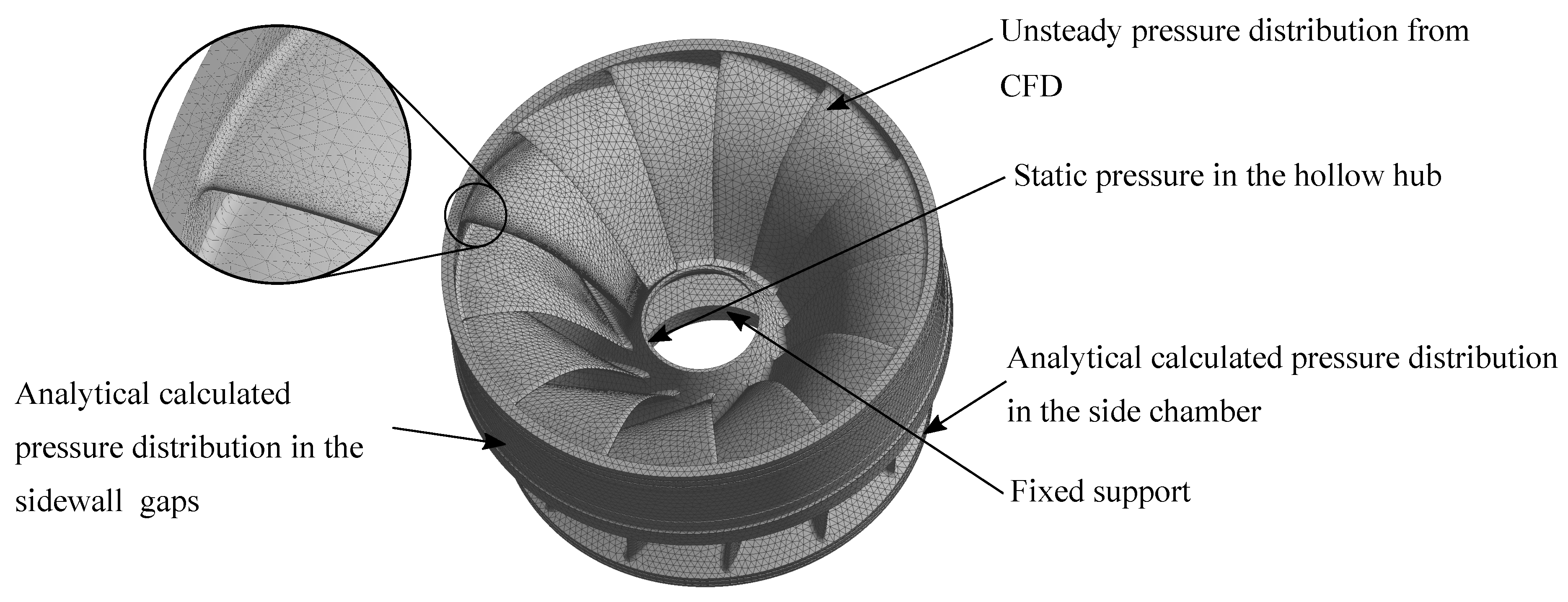
3.3. FEM-Setup

3.3.1. Modal Analysis

ANSYS-Mechanical 18.1 was used to perform the modal analysis and to calculate the natural frequencies and mode shapes. Figure 5 shows the considered draft tube model including concrete and water volume.

The fluid volume was created by the use of acoustic elements and the nodes on the interface are conformal with the ones of the structural domain. Moreover, the concrete volume and the draft tube as well as the manhole cover are connected by a ridges contact elements ensuring no damping. At the outer surfaces the concrete volume was fixed, while at the draft tube inlet and outlet a constant pressure was applied. The whole model consists of about 731,000 elements and 488,000 nodes [35].

3.3.2. Transient FEM Analysis

Besides the flow simulations, the purpose of the investigation is to evaluate the dynamical runner stress. Therefore, Figure 6 shows the transient FEM setup including boundary conditions. The runner is fixed at the bold cycle, gravitational and centrifugal forces as well as a mean static pressure value at the hollow hub is applied. The whole tetrahedral mesh consists of about 0.7 m nodes including a partial refinement at one specific blade, where the strain gauges are located. To capture the highest dynamical stress obtained at the location of $S2$, the mean value of the nodes covered by the strain gauge was calculated. A total number of six runner revolutions is simulated with a time step corresponding to a runner rotation of $3^{\circ }$.

Due to different mesh requirements for flow and structural simulations a mapping algorithm is required to transfer the pressure fields. According to the literature, different algorithms have been compared to each other revealing a recommendation of the Gauss integration [36]. However, the nearest neighbour method [37] transferring data to the closest node of the structural mesh is the most simple and fastest approach. In order to improve the accuracy of this method without significantly increasing the calculation time, an orthogonal projection algorithm can be applied [36]. Instead of taking the value of the closest node, the considered fluid node is projected on the structural mesh and the reconstructed value of the quantity of interest is used. In terms of the coupling, one-way or two-way fluid structure interaction (FSI) can be applied. Although two way FSI is closer to reality where structural deformations will also impact the flow, it has been shown that in case of Francis turbines the results of one-way and two-way FSI are similar [38]. The already high computational times and resources demanding transient FEM considering a similar approach as shown in [39] would increase significantly by the use of a two-way coupling. Therefore, a one-way fluid structure coupling and the nearest neighbour orthogonal projection approach is applied. Moreover, the flow in the sidewall gaps has not been considered in the CFD calculations. However, in the FEM analysis the pressure distribution calculated by means of an analytical model is applied on hub and shroud of the runner. The model is originally based on the leakage flow calculation approach of Gülich [40] and the modifications are described and validated in [41]. Another important factor for the accuracy of the FEM model is the damping of the structure. Therefore a simplified approach specifying an equivalent Rayleigh damping according to

$$\left[C_D\right]=\alpha \left[M\right]+\beta \left[K\right]$$

(4)

in which $\left[C_D\right]$ describes the damping matrix, $\left[M\right]$ the mass matrix and $\left[K\right]$ the stiffness matrix of the runner is applied. The Rayleigh coefficients $\alpha$ and $\beta$ can be determined by an approach proposed by Clough et al. [42] with

$$\left\{\begin{array}{c}\alpha \\ \beta \end{array}\right\}=\frac{2{\omega }_1{\omega }_2}{{{\omega }_2}^2-{{\omega }_1}^2}\left[\begin{array}{cc}{\omega }_2& -{\omega }_1\\ -\frac{1}{{\omega }_2}& \frac{1}{{\omega }_1}\end{array}\right]\left\{\begin{array}{c}\zeta \\ \zeta \end{array}\right\}$$

(5)

in which $\omega$ determines the frequency limit and $\zeta$ the damping ratio.

Table 2. Frequency limits and resulting damping coefficients.

Description Parameters	Parameters
Damping ratio $\zeta$ (-)	$0.01$
Low limit frequency $f_1$ (Hz)	1
Upper limit frequency $f_2$ (Hz)	$344.2$
Rayleigh coefficient $\alpha$ (-)	$0.1253$
Rayleigh coefficient $\beta$ (-)	$9.2216\times {10}^{-6}$

summarizes the parameters and used values. The upper limit frequency $f_2$ related to the angular eigenfrequency based on the cumulative mass participation as suggested by Chowdhury [43], while the lower limit frequency $f_1$ is extended beneath $f_0$ to cover the whole low frequency band. As described in [44] the actual damping ratio $\zeta$ is hard to obtain with high accuracy and is often based on limited experimental knowledge. Therefore, a reasonable value based on the literature [45,46] is chosen.

3.4. Life Expectancy

Based on the static and dynamic stresses at the hotspots, relative or absolute lifetime can be calculated. Therefore the rainflow counting algorithm is used to determine the load spectra. To compare the simulated stress amplitudes to the measured signal an extrapolation as suggested by Johannesson [47] is used. On the extreme value theory based approach, this has already been successfully applied in case of load spectra of Francis turbine runners [22,39]. However, to determine runner fatigue damage, material properties have to be included. The classical fatigue method uses an S-N curve as an initial guess, where runner fatigue may occur. This S-N curve is dependant on test results of a probe and as a result not considering the impact of previous loads. Therefore, it can only be used for a relative damage lifetime prediction.

Table 3. Material Data.

Description Parameters	Parameters
Material (-)	$X5$$Cr$$Ni$ 13 4
Survival probability (%)	$99.99$
Mean stress (N/mm${}^2$)	150
Logarithmic standard deviation of ${\sigma }_a$ (-)	$0.07$
Stress ratio (-)	1

shows the used material properties based on a internal test report for samples in water. Furthermore, the Miner’s rule can be used to calculate a damage factor

$$C=\frac{n_i}{N_i}$$

(6)

with $n_i$ the number of cycles and $N_i$ those necessary to produces failure referring to the S-N curve. According to the definition, failure is occurring if $C=1$. Although this approach is widely used for fatigue assessments by academic and industrial researches, it is not suitable to treat crack growth and consider the influence of high cycle fatigue onset. Consequently, Gagnon et al. [48,49] proposed a more complex way according to the linear elastic fracture mechanics. However, the paper limits itself to an improvement of the numerical methodology and comparison with air injection. Moreover, no cracks have been detected during acceptance tests. Therefore, the simplified approach is used to access fatigue damage.

4. Results and Discussion

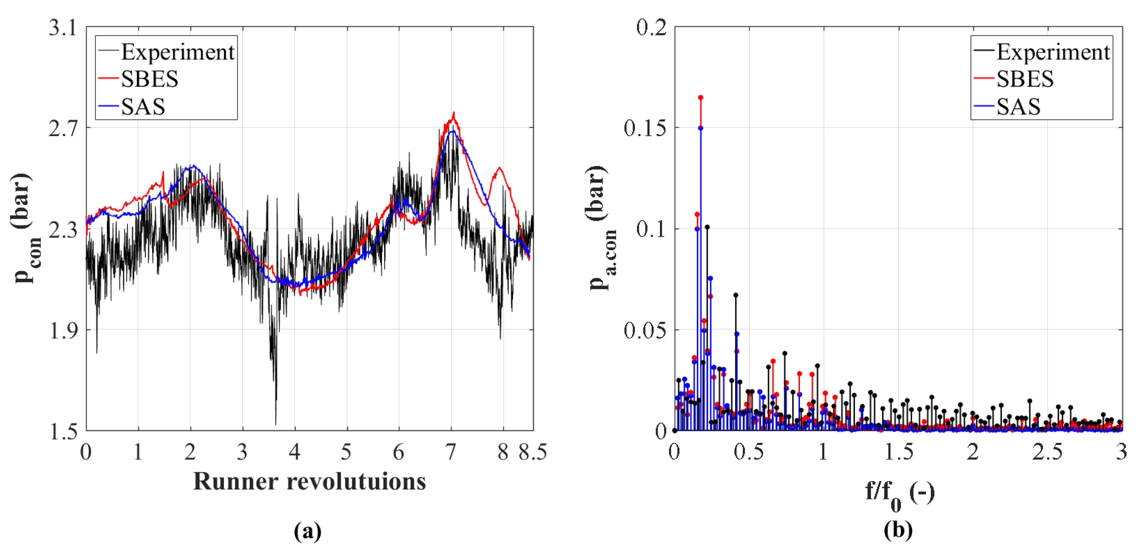
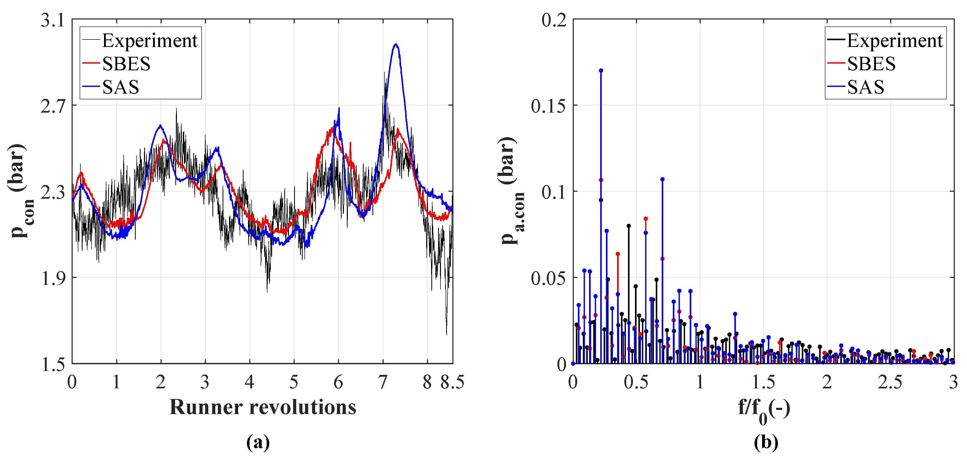
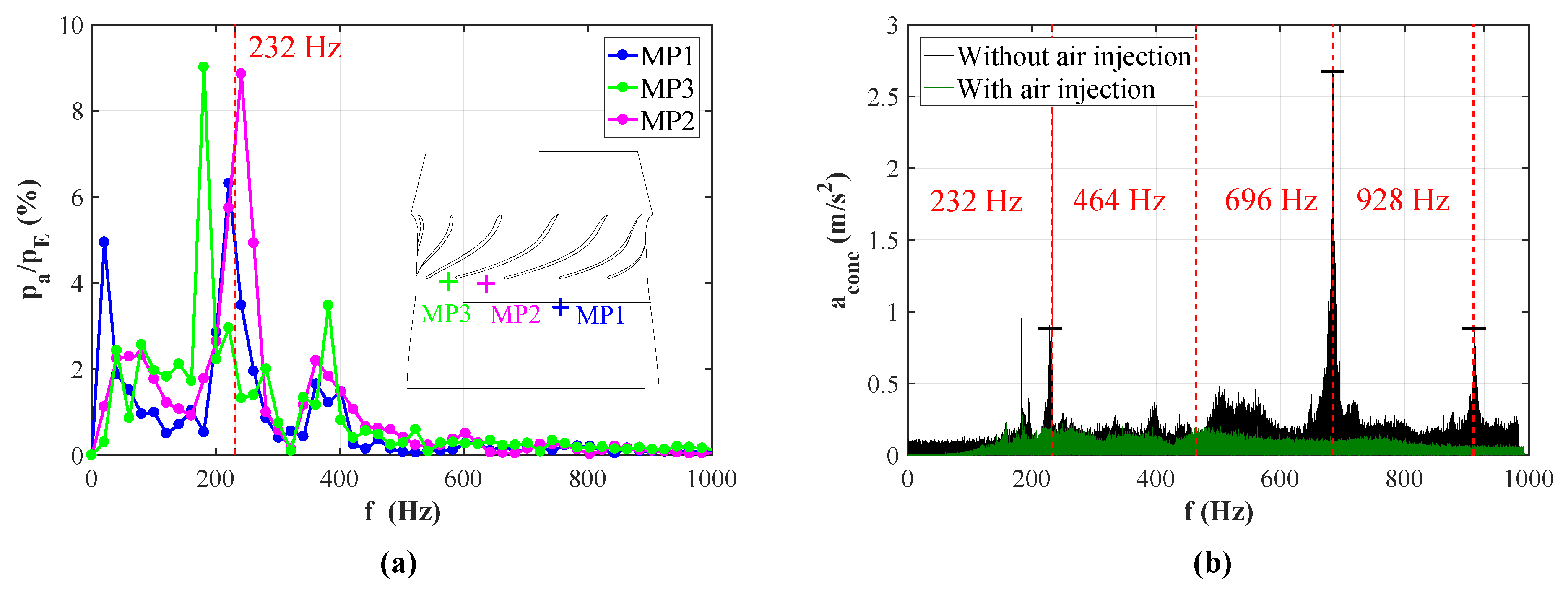
4.1. Cavitation Behavior and Pressure Oscillations

The pressure signals without air injection of the transducer $p_{con}$ are compared to the numerical results in Figure 7. The left-hand side shows a duration of $8.5$ runner revolutions, corresponding to approximately one and a half principal oscillations of the signal (Figure 7a). Both turbulence models produce similar results and predict the signal relatively well based on the pressure oscillation induced by the draft tube vortex. However, oscillations in the higher frequency range are neither fully captured by the SAS model nor by the SBES, which produces more LES regions. The time step and the grid resolution are certainly limiting factors in this regard. Looking at the frequency spectrum shown in Figure 7b, it can be seen that the model captures the phenomenon but clearly overestimates the pressure pulsations, which is a common problem of the cavitation model, reported in the literature [50]. In the simulation as well as in the experiment, a distinctive harmonic frequency peak at approximately $f=0.2·f_0$, corresponding to a draft tube vortex rotation, can be determined. The vortex rotation frequency is slightly lower in the simulation than in the measurement. The application of the SBES model leads to slightly higher pressure amplitudes and higher computational times. Therefore, to capture pressure pulsations in the draft tube the SAS model is the slightly better choice.

Furthermore, Figure 8 shows the impact of the air injection on the pressure pulsations in the draft tube. The integration of air as the second medium in the simulation leads to higher computational times compared to the previous discussed case. The time signal obtained by the transducer $p_{con}$ with air (Figure 7a) oscillates still in the same waveform than without air. In case of the amplitude a clear overestimation with slightly better results of the SBES model can be seen.

Moreover, the use of the aeration system does not influence the amplitude of the pressure pulsations measured by $p_{con}$. Figure 9a highlights vortex structures in the draft tube using the Q-criterion, colored by the turbulent kinetic energy k. The simulation can reproduce the draft tube vortex and indicates the appearance of smaller vortex structures starting from the trailing edge. Additionally, in Figure 9b the results considering air injection are depicted. The magenta colored iso-surface is showing the regions, where the concentration of air is more than $2\%$. This is basically the case around the runner walls. Especially near the shroud, the air concentration is higher than anywhere else.

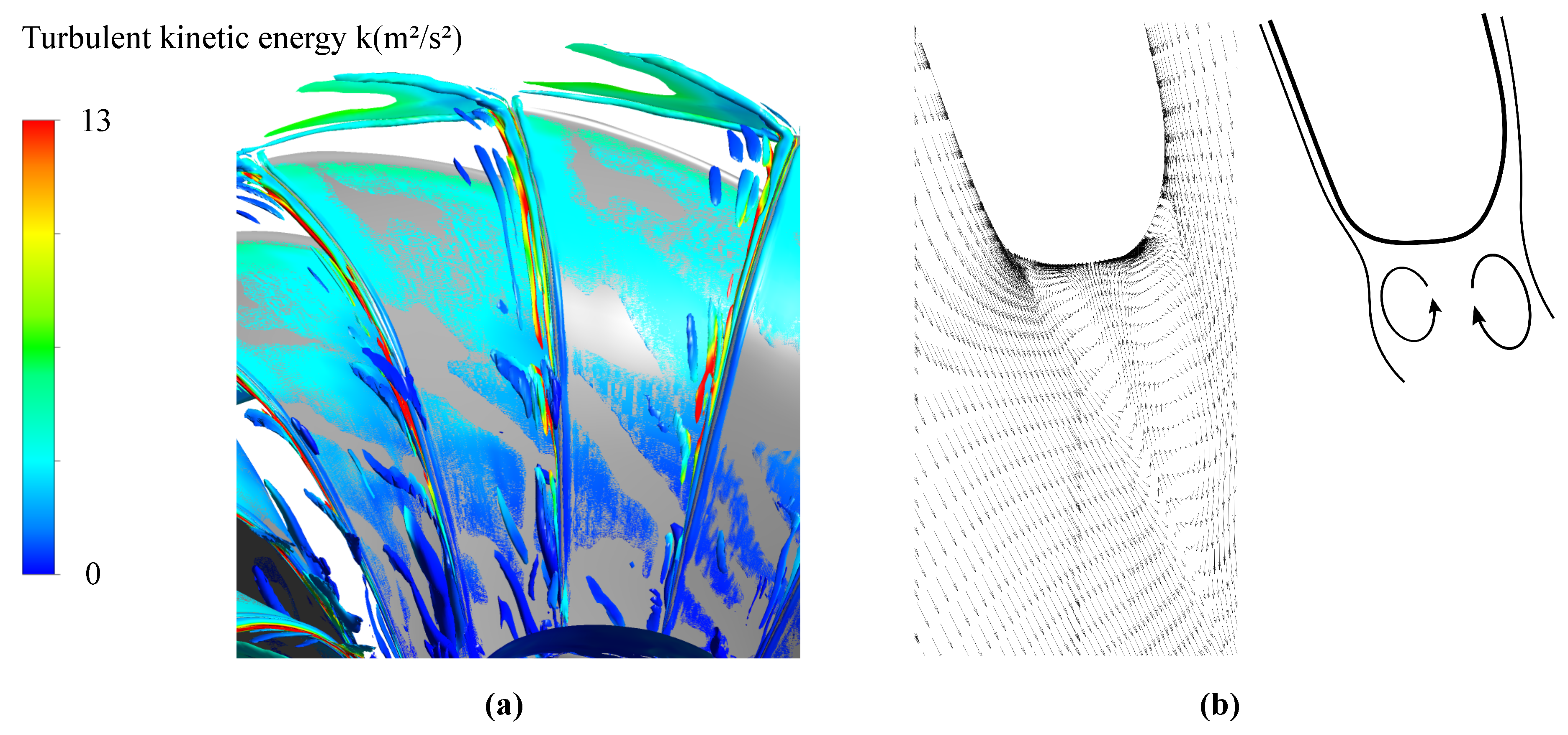
4.2. Trailing Edge Vortex Shedding

As shown in Figure 3 the machine set suffers under high vibration and noise around $50\%$ of $P_{RP}$ without aeration. Based on the vibration measurements a distinctive fundamental frequency of approximately 230 Hz was discovered. Due to the fact that this frequency neither depends on $f_0$ nor on the draft tube vortex, the appearance of a trailing edge vortex shedding can be assumed. Although this effect is usually common at the stay or guide vanes of Francis turbines [51,52], some cases of runner trailing edge vortex shedding are reported in the literature as well [53]. Analytically the frequency of eddy detachment can be determined by the Strouhal number (St). The vortex shedding frequency can be expressed by

$$f_{SV}=\frac{St·v}{L}$$

(7)

where v is the velocity and L is the characteristic lateral dimension. The coefficient is originally calculated for a cylinder in free stream, but is also used for turbine blades. Regarding hydraulic turbines it mainly depends on the Reynolds number (Re) and the shape of the blade leading to uncertainties of the relation. To evaluate the possibility of vortex shedding, a frequency $f_{SV}$ is calculated by using the trailing edge thickness L and an analytical calculated relative velocity at the runner outlet. The consideration of a reasonable Strouhal number $St=0.2$, results in a detachment frequency $f_{SV}\approx 235$ Hz. This highly indicates a relation between the draft tube excitation and trailing edge vortex shedding. Therefore, further CFD simulations using the RN VS domain are performed. Due to the possibility of directly forcing LES behavior by grid refinement in certain location, the SBES model was chosen to approximate turbulence. Figure 10a shows the discovered vortex shedding on the runner trailing edge by means of the Q-criterion and colored by the turbulent kinetic energy k. The effect propagates in spanwise-direction of the trailing edge, but is especially clearly visible near the shroud. Figure 10b shows the blade-to-blade velocity vector plot, highlighting the rotation direction of the vortices.

To determine the excitation frequency several monitor points (MPs) in the draft tube cone close to the runner are applied in the CFD simulation. Furthermore, these signals are transposed to the frequency domain by the use of a fast Fourier transform (FFT) algorithm. Figure 11a shows, the pressure oscillations captured by three circumferential distributed monitor points normalized by the pressure corresponding to the circumferential velocity referred to the outer diameter of runner outlet

$$p_E={\rho }_f·\frac{u_2^2}{2}$$

(8)

According to Figure 11a there are significant peaks occurring at 190 Hz, 220 Hz and 240 Hz, related to the eddy detachment. Moreover, it is described by Koopmann [54] that the vortex shedding frequency can synchronize with the natural frequency of the structure. Even if the flow conditions are unsteady the frequency remains “locked-in” until the frequency deviation becomes too large. Figure 11b shows the structural response of the draft tube by means of the vibration sensor $a_{con}$ without (black) and with aeration (green). Without air injection a fundamental harmonic peak is appearing at approximately 232 Hz, while the second frequency is not clearly visible. However, the highest peak is appearing at 696 Hz which corresponds to the third harmonic of the fundamental frequency. In case of the air admission, those frequency peaks vanish completely. Only slightly beneath 200 Hz small peaks are visible. This corresponds well with the results shown in Figure 9b, which shows the air distribution in the runner. Besides adding global damping effects the air is gathering around hub and shroud side of the runner. Further downstream the highest air volume concentration is in the boundary layer of the draft tube. Consequently, the air admission is not only impeding the formation of the vortex shedding but is shielding the runner blade against induced pressure pulsations.

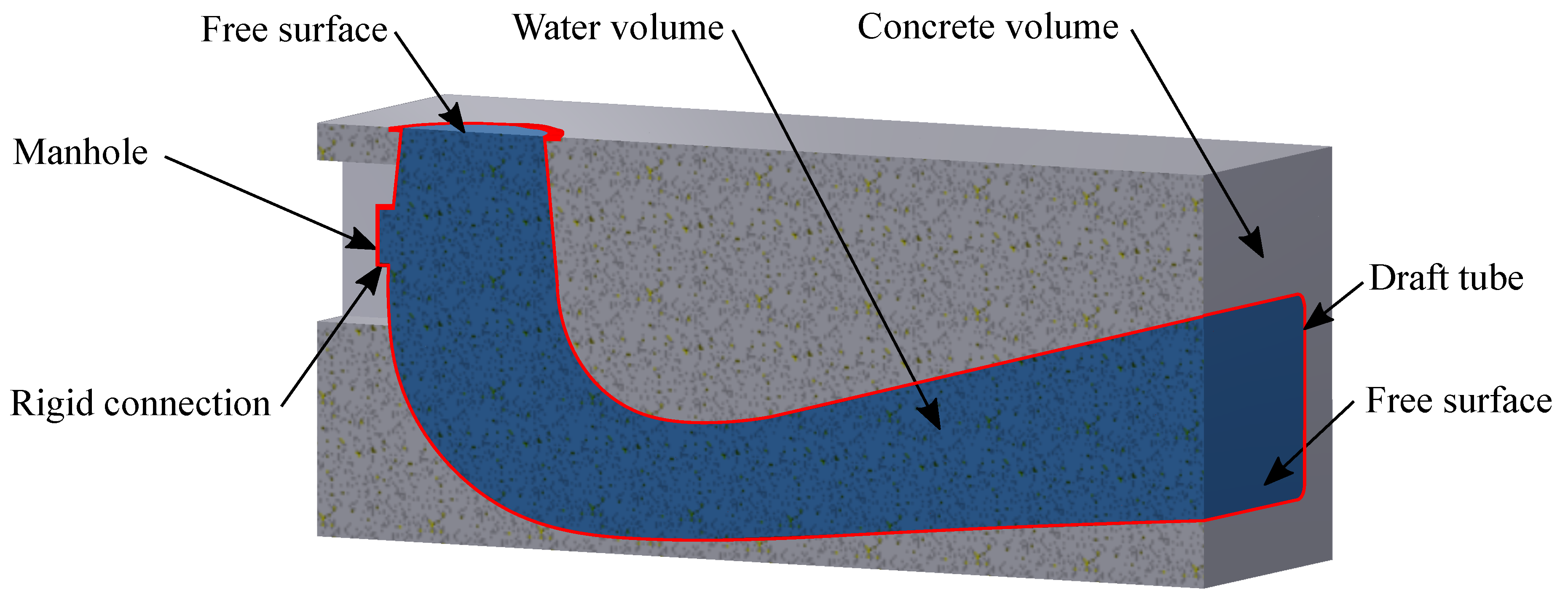
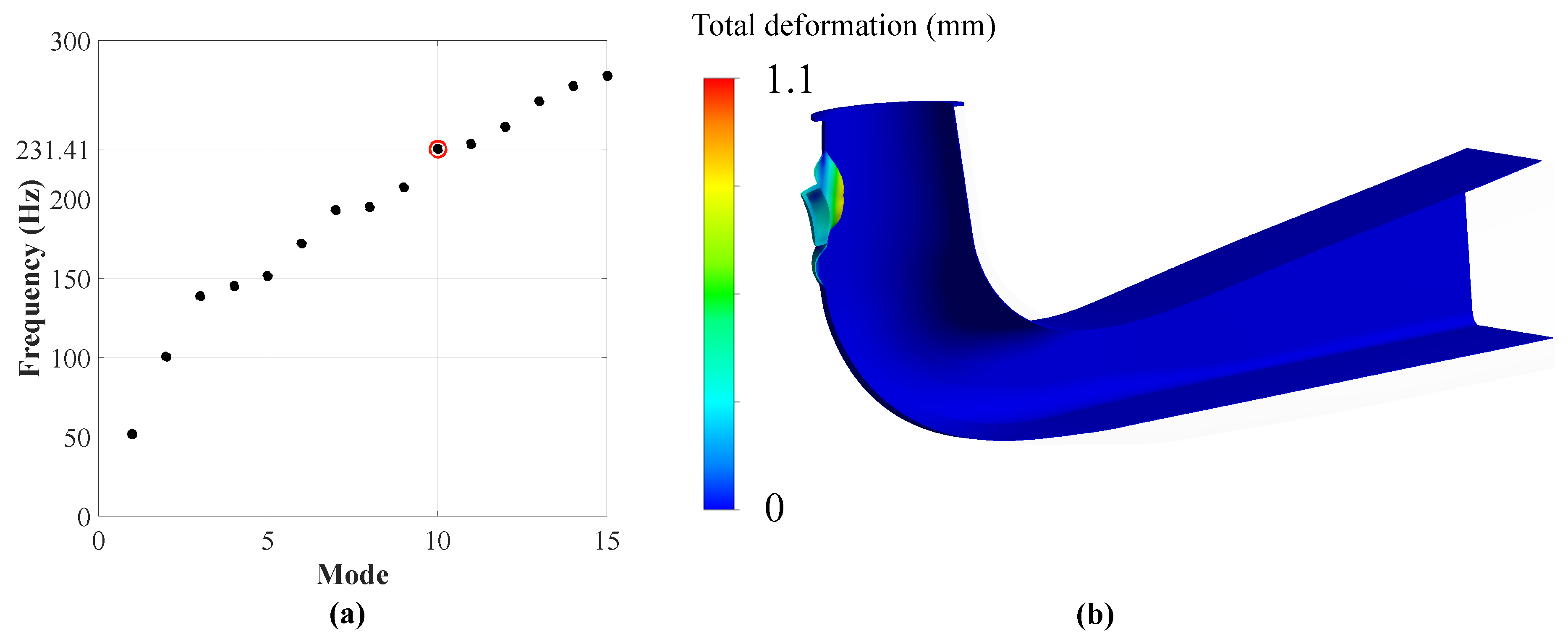
4.3. Modal Analysis of the Draft Tube

After discovering the excitation mechanism the corresponding natural frequency must be determined, in order to clarify whether or not resonance is occurring. Therefore, a modal analysis of the draft tube, taking concrete and water volume into account, is carried out. In Figure 12a the first 15 modes can be seen. It appears that the numerical simulation predicts a natural frequency close to the excitation frequency discovered by CFD analysis and vibration measurements. According to Figure 12a the closest natural frequency appears at 231.41 Hz which corresponds to the excitation mechanism shown in Figure 11.

Most of the deformation takes place at the concrete-free area, where the manhole is located (Figure 12b).

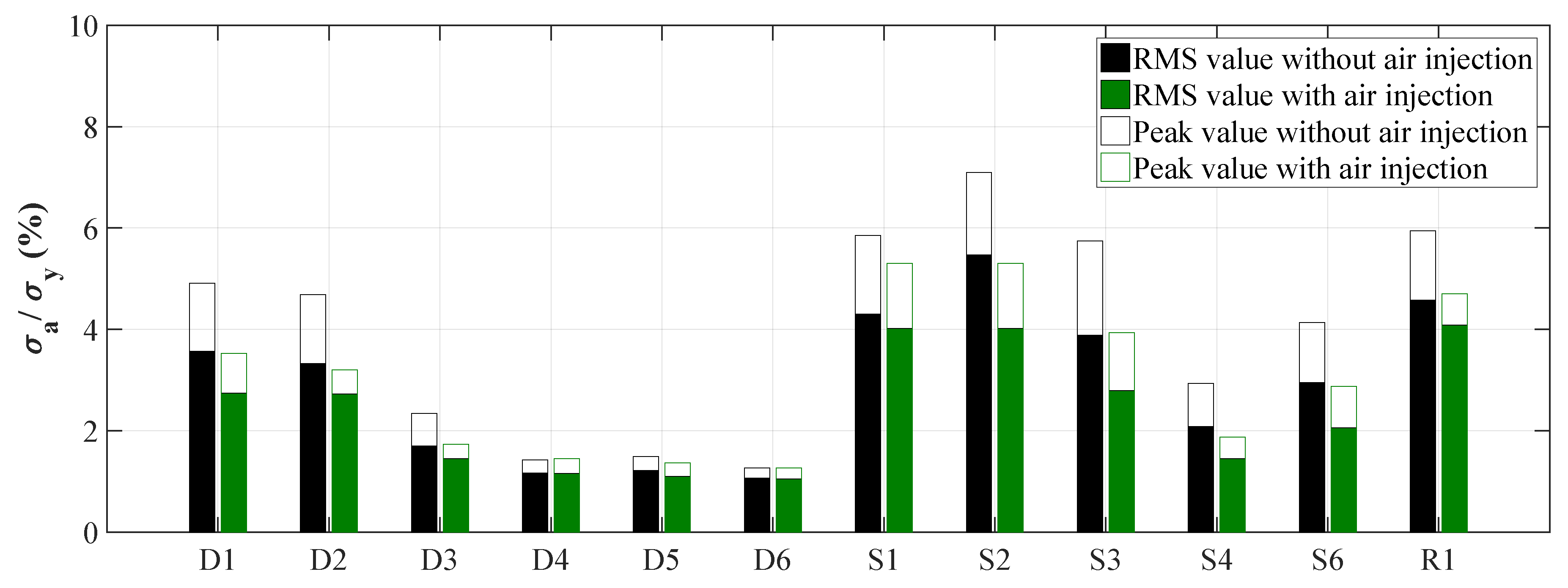
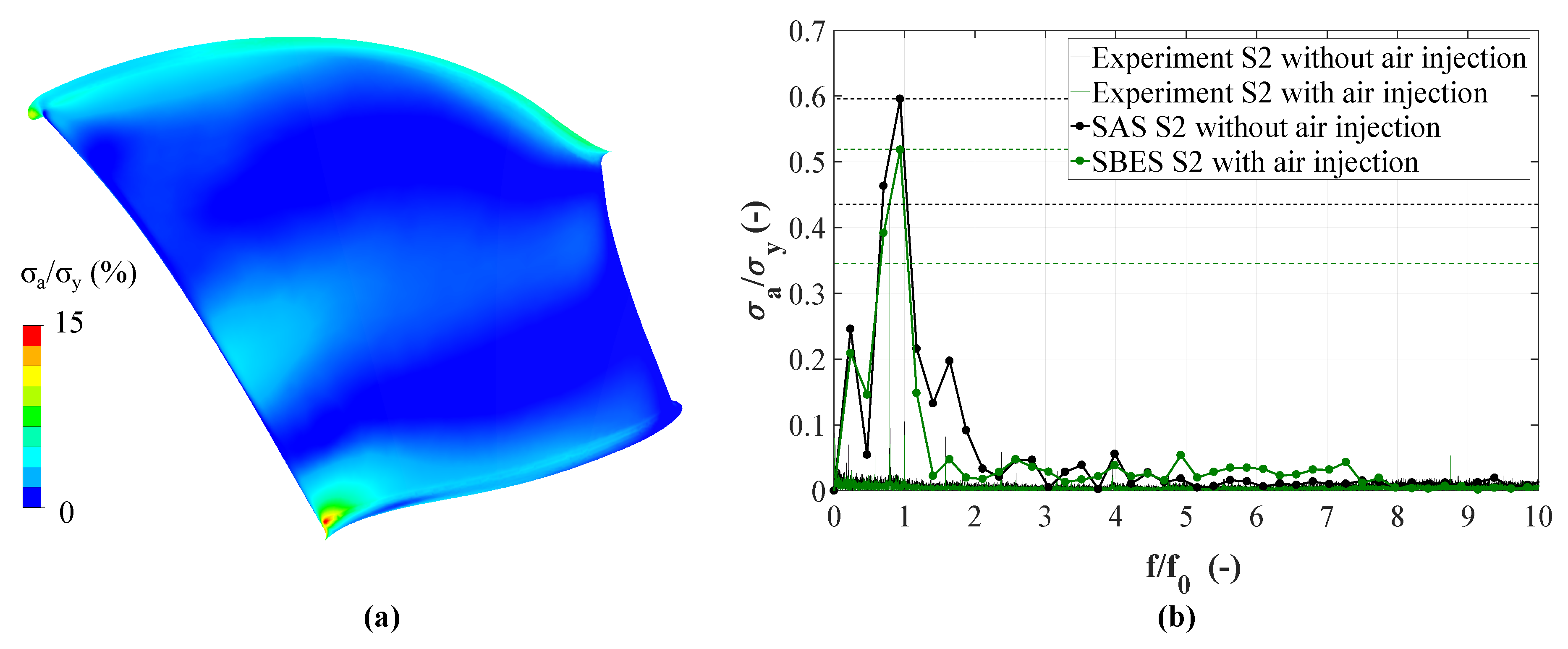
4.4. Fatigue Damage and Dynamical Stress

Based on the strain gauge measurement the influence of the air injection on the runner stress root mean square (RMS) and peak values can be seen in Figure 13. Contrary to the pressure pulsations in the draft tube cone the runner stress decreases. Especially, at the critical location of S2 the stress is reduced by approximately $25\%$ of the initial value.

According to the presented FEM setup a transient FEM simulation was done for both cases. The von Mises stress distribution of one time step without aeration is shown in Figure 14a. The maximum value is located close to $S2$, which corresponds well to the experimental results depicted in Figure 13. On the right-hand side (Figure 14b), the stress based on experimental and numerical data at the location of $S2$ is shown. Due to reasons of clarity and because both turbulence models produced very similar results, only the slightly better choice is displayed in the frequency domain. Although the resolution is much coarser the numerical simulation can reproduce the highest peak at approximately $0.8·f_0$, corresponding to the draft tube vortex measured in the relative system.

The load spectra for both cases are depicted in Figure 15. On the left-hand side the results of the SAS and the SBES model are compared to the experimental results without aeration (Figure 15a), whereas on the right-hand side the cases considering air injection (Figure 15b) are presented. Contrary to the pressure pulsation in Section 4.1 the simulated load-spectra without air injection are lower than the measured one. However, a compartment to Figure 15b shows that the stress amplitudes obtained by the simulation do not decrease as much as in the experiment.

5. Conclusions

The main topic of this study was to investigate the critical load region of a prototype Francis turbine by means of site measurements and simulations. The measurements showed significant high vibrations around $44\%$ of the rated power. Therefore, a CFD analysis by the use of two hybrid turbulence models (SAS, SBES) was performed. The high frequency pressure measurement in the draft tube ($p_{con}$) was used to validate the results of the CFD analysis. The key results can be summarized as follows:

• A huge draft tube vortex, with a frequency corresponding to approximately $0.2·f_0$, is the most concerning fact in terms of high dynamical stress and runner fatigue damage.
• Both turbulence models showed quite similar behavior and a good agreement with the measurement. However, in contrast to single flow analysis the pressure amplitudes of the simulation tend to be higher than the ones obtained by the sensor.
• An improved runner model, targeting separation effects, showed the appearance of trailing edge vortex shedding.
• A simplified modal analysis of the draft tube confirmed that the vibrations of the machine set are related to vortex shedding.
• The air injection not only significantly reduced the vibrations of the machine set and might have a positive effect on cavitation, but also improved runner fatigue life.

The numerical approach accurately predicts the stress amplitudes in the case without air injection but needs to be further improved to sufficiently handle the decrease of the dynamical stress. In this regard, it would be an improvement to take the compressibility of the air phase into account. Regarding the draft tube excitation, further numerical and experimental investigations considering the complexity of the whole system are planned. Consequently, additional air injection through the hub might be tested and would most likely disturb the draft tube vortex core and therefore further improve the runner behavior in the critical low load region. In terms of the numerical approach, the cavitation model, depending on fixed empirical values with influence on the vapor volume (like the mean nucleation site diameter) is the main source of uncertainty and needs to be further validated.

References

- Trivedi, C.; Gandhi, B.; Michel, C.J. Effect of transients on Francis turbine runner life: A review. J. Hydraul. Res. 2013, 51, 121–132. [Google Scholar] [CrossRef]
- Yamamoto, K.; Müller, A.; Favrel, A.; Avellan, F. Experimental evidence of inter-blade cavitation vortex development in Francis turbines at deep part load condition. Exp. Fluids 2017, 58, 142. [Google Scholar] [CrossRef]
- Goyal, R.; Gandhi, B.K. Review of hydrodynamics instabilities in Francis turbine during off-design and transient operations. Renew. Energy 2018, 116, 697–709. [Google Scholar] [CrossRef]
- Xiao, R.; Wang, Z.; Luo, Y. Dynamic stresses in a Francis turbine runner based on fluid-structure interaction analysis. Tsinghua Sci. Technol. 2008, 13, 587–592. [Google Scholar] [CrossRef]
- Trudel, A.; Sabourin, M. Metallurgical and Fatigue Assessments of Welds in Cast Welded Hydraulic Turbine Runners. IOP Conf. Ser. Earth Environ. Sci. 2014, 22, 012015. [Google Scholar] [CrossRef]
- Rheingans, W. Power swings in hydroelectric power plants. Trans. ASME 1940, 62, 171–184. [Google Scholar]
- Seidel, U.; Mende, C.; Hübner, B.; Weber, W.; Otto, A. Dynamic Loads in Francis Runners and Their Impact on Fatigue Life. IOP Conf. Ser. Earth Environ. Sci. 2014, 22, 032054. [Google Scholar] [CrossRef]
- Egusquiza, E.; Valero, C.; Huang, X.; Jou, E.; Guardo, A.; Rodriguez, C. Failure investigation of a large pump-turbine runner. Eng. Fail. Anal. 2012, 23, 27–34. [Google Scholar] [CrossRef]
- Frunzăverde, D.; Muntean, S.; Mărginean, G.; Campian, V.; Marşavina, L.; Terzi, R.; Şerban, V. Failure Analysis of a Francis Turbine Runner. IOP Conf. Ser. Earth Environ. Sci. 2010, 12, 012115. [Google Scholar] [CrossRef]
- Thicke, R. Practical solutions for draft tube instability. Water Power Dam Constr. 1981, 32, 31–37. [Google Scholar]
- Qian, Z.; Li, W.; Huai, W.; Wu, Y. The effect of runner cone design on pressure oscillation characteristics in a Francis hydraulic turbine. Proc. Inst. Mech. Eng. Part A J. Power Energy 2012, 226, 137–150. [Google Scholar] [CrossRef]
- Dörfler, P.; Sick, M.; Coutu, A. Flow-Induced Pulsation and Vibration in Hydroelectric Machinery: Engineer’s Guidebook for Planning, Design and Troubleshooting; Springer Science & Business Media: Berlin/Heidelberg, Germany, 2012. [Google Scholar]
- Muntean, S.; Susan-Resiga, R.F.; Câmpian, V.C.; Dumpravă, C.; Cuzmoş, A. In situ unsteady pressure measurements on the draft tube cone of the Francis turbine with air injection over an extended operating range. UPB Sci. Bull. Ser. D 2014, 76, 173–180. [Google Scholar]
- Nakanishi, K.; Ueda, T. Air supply into draft tube of Francis turbine. Fuji Electr. Rev. 1964, 10, 81–91. [Google Scholar]
- March, P. Hydraulic and environmental performance of aerating turbine technologies. In EPRI-DOE Conference on Environmentally-Enhanced Hydropower Turbines: Technical Papers; EPRI: Palo Alto, CA, USA; U.S. Department of Energy: Washington, DC, USA, 2011; pp. 19–21. [Google Scholar]
- Dörfler, P.; Bloch, R.; Mayr, W.; Hasler, O. Vibration tests on a high-head (740 m) Francis turbine: Field test results from Hausling. In Proceedings of the 14th IAHR Symposium on Hydraulic Machinery and Cavitation, Trondheim, Norway, 20–23 June 1988; pp. 241–252. [Google Scholar]
- Von Fellenberg, S.; Häussler, W.; Michler, W. High-Pressure Air Injection on a Low-Head Francis Turbine. IOP Conf. Ser. Earth Environ. Sci. 2014, 22, 012031. [Google Scholar] [CrossRef]
- Zhang, Y.; Zheng, X.; Li, J.; Du, X. Experimental study on the vibrational performance and its physical origins of a prototype reversible pump turbine in the pumped hydro energy storage power station. Renew. Energy 2019, 130, 667–676. [Google Scholar] [CrossRef]
- Chen, T.; Zhang, Y.; Li, S. Instability of large-scale prototype Francis turbines of Three Gorges power station at part load. Proc. Inst. Mech. Eng. Part A J. Power Energy 2016, 230, 619–632. [Google Scholar] [CrossRef]
- Chirkov, D.; Shcherbakov, P.; Cherny, S.; Skorospelov, V.; Turuk, P. Numerical investigation of the air injection effect on the cavitating flow in Francis hydro turbine. Thermophys. Aeromech. 2017, 24, 691–703. [Google Scholar] [CrossRef]
- Unterluggauer, J.; Doujak, E.; Bauer, C. Numerical fatigue analysis of a prototype Francis turbine runner in low-load operation. In Proceedings of the European Turbomachinery Conference, Laussanne, Switzerland, 8–12 April 2019; pp. 1–12. [Google Scholar]
- Eichhorn, M.; Taruffi, A.; Bauer, C. Expected load spectra of prototype Francis turbines in low-load operation using numerical simulations and site measurements. J. Phys. Conf. Ser. 2017, 813, 012052. [Google Scholar] [CrossRef]
- International Electrotechnical Commission. Hydraulic Turbines, Storage Pumps and Pump-Turbines-Model Acceptance Tests: IEC 60193: 1999; International Electrotechnical Commission: Geneva, Switzerland, 1999. [Google Scholar]
- Unterluggauer, J.; Doujak, E.; Bauer, C. Fatigue analysis of a prototype Francis turbine based on strain gauge measurements. In 20th International Seminar on Hydropower Plants; Technische Universität Wien Eigenverlag: Vienna, Austria, 2018. [Google Scholar]
- Papillon, B.; Sabourin, M.; Couston, M.; Deschenes, C. Methods for air admission in hydro turbines. In Proceedings of the 21st IAHR Symposium on Hydraulic Machinery and Systems, Lausanne, Switzerland, 9–12 September 2002; pp. 1–6. [Google Scholar]
- Qian, Z.D.; Yang, J.D.; Huai, W.X. Numerical simulation and analysis of pressure pulsation in Francis hydraulic turbine with air admission. J. Hydrodyn. 2007, 19, 467–472. [Google Scholar] [CrossRef]
- Celik, B.; Ghia, U.; Roache, P.; Freitas, C.; Coleman, H.; Raad, P. Procedure for Estimation and Reporting of Uncertainty Due to Discretization in CFD Applications. J. Fluids Eng. 2008, 130, 78001. [Google Scholar] [CrossRef]
- Menter, F. Zonal two equation k-w turbulence models for aerodynamic flows. In Proceedings of the 23rd Fluid Dynamics, Plasma Dynamics, and Lasers Conference, Orlando, FL, USA, 6–9 July 1993; p. 2906. [Google Scholar]
- Menter, F.; Egorov, Y. The scale-adaptive simulation method for unsteady turbulent flow predictions. Part 1: Theory and model description. Flow Turbul. Combust. 2010, 85, 113–138. [Google Scholar] [CrossRef]
- Menter, F. Stress-Blended Eddy Simulation (SBES)—A New Paradigm in Hybrid RANS-LES Modeling. In Symposium on Hybrid RANS-LES Methods; Springer: Berlin/Heidelberg, Germany, 2016; pp. 27–37. [Google Scholar]
- Menter, F. Stress-Blended Eddy Simulation (SBES)—A New Paradigm in Hybrid RANS-LES Modeling. In Progress in Hybrid RANS-LES Modelling; Hoarau, Y., Peng, S.H., Schwamborn, D., Revell, A., Eds.; Springer International Publishing: Cham, Switzerland, 2018; pp. 27–37. [Google Scholar]
- Plesset, M.S.; Prosperetti, A. Bubble dynamics and cavitation. Annu. Rev. Fluid Mech. 1977, 9, 145–185. [Google Scholar] [CrossRef]
- Bakir, F.; Rey, R.; Gerber, A.; Belamri, T.; Hutchinson, B. Numerical and experimental investigations of the cavitating behavior of an inducer. Int. J. Rotating Mach. 2004, 10, 15–25. [Google Scholar] [CrossRef]
- Mössinger, P.; Conrad, P.; Jung, A. Transient Two-Phase CFD Simulation of Overload Pressure Pulsation in a Prototype Sized Francis Turbine Considering the Waterway Dynamics. IOP Conf. Ser. Earth Environ. Sci. 2014, 22, 032033. [Google Scholar] [CrossRef]
- Nocker, A. Modal Analysis of a Concreted Draft Tube of a Francis Machine. Bachelor’s Thesis, Technical University of Vienna, Vienna, Austria, 2019. [Google Scholar]
- De Boer, A.; van Zuijlen, A.H.; Bijl, H. Comparison of conservative and consistent approaches for the coupling of non-matching meshes. Comput. Methods Appl. Mech. Eng. 2008, 197, 4284–4297. [Google Scholar] [CrossRef]
- Thévenaz, P.; Blu, T.; Unser, M. Interpolation revisited [medical images application]. IEEE Trans. Med. Imaging 2000, 19, 739–758. [Google Scholar] [CrossRef] [PubMed]
- Zhu, W.; Xiao, R.; Yang, W.; Liu, J.; Wang, F. Study on Stress Characteristics of Francis Hydraulic Turbine Runner Based on Two-Way FSI. IOP Conf. Ser. Earth Environ. Sci. 2012, 15, 052016. [Google Scholar] [CrossRef]
- Morissette, J.; Chamberland-Lauzon, J.; Nennemann, B.; Monette, C.; Giroux, A.; Coutu, A.; Nicolle, J. Stress Predictions in a Francis Turbine at No-Load Operating Regime. IOP Conf. Ser. Earth Environ. Sci. 2016, 49, 072016. [Google Scholar] [CrossRef]
- Gülich, J.F. Centrifugal Pumps; Springer: Berlin/Heidelberg, Germany, 2008; Volume 2. [Google Scholar]
- Maly, A.; Eichhorn, M.; Bauer, C. Experimental investigation of transient pressure effects in the side chambers of a reversible pump turbine model. In 19. Internationales Seminar Wasserkraftanlagen//19th International Seminar on Hydropower Plants; Technische Universität Wien, Ed.; Technische Universität Wien Eigenverlag: Vienna, Austria, 2016; pp. 675–684. [Google Scholar]
- Clough, R.W.; Penzien, J. Dynamics of Structures; Computers & Structures, Inc.: Berkeley, CA, USA, 1995. [Google Scholar]
- Chowdhury, I.; Dasgupta, S.P. Computation of Rayleigh damping coefficients for large systems. Electron. J. Geotech. Eng. 2003, 8, 1–11. [Google Scholar]
- Rodriguez, C.; Egusquiza, E.; Escaler, X.; Liang, Q.; Avellan, F. Experimental investigation of added mass effects on a Francis turbine runner in still water. J. Fluids Struct. 2006, 22, 699–712. [Google Scholar] [CrossRef]
- Magnoli, M.V. Numerical Simulation of Pressure Oscillations in Large Francis Turbines at Partial and Full Load Operating Conditions and Their Effects on the Runner Structural Behaviour and Fatigue Life. Ph.D. Thesis, Technische Universität München, Munich, Germany, 2014. [Google Scholar]
- Flores, M.; Urquiza, G.; Rodríguez, J.M. A fatigue analysis of a hydraulic Francis turbine runner. World J. Mech. 2012, 2, 28–34. [Google Scholar] [CrossRef]
- Johannesson, P. Extrapolation of load histories and spectra. Fatigue Fract. Eng. Mater. Struct. 2006, 29, 209–217. [Google Scholar] [CrossRef]
- Gagnon, M.; Tahan, S.; Bocher, P.; Thibault, D. The Role of High Cycle Fatigue (HCF) Onset in Francis Runner Reliability. IOP Conf. Ser. Earth Environ. Sci. 2012, 15, 022005. [Google Scholar] [CrossRef]
- Thibault, D.; Gagnon, M.; Godin, S. The effect of materials properties on the reliability of hydraulic turbine runners. Int. J. Fluid Mach. Syst. 2015, 8, 254–263. [Google Scholar] [CrossRef]
- Jošt, D.; Škerlavaj, A.; Morgut, M.; Nobile, E. Numerical prediction of cavitating vortex rope in a draft tube of a Francis turbine with standard and calibrated cavitation model. J. Phys. Conf. Ser. 2017, 813, 012045. [Google Scholar] [CrossRef]
- Goldwag, E.; Berry, D. Von Karman hydraulic vortexes cause stay vane cracking on propeller turbines at the little long generating station of Ontario hydro. J. Eng. Power 1968, 90, 213–217. [Google Scholar]
- Trivedi, C. Compressible large eddy simulation of a Francis turbine during speed-no-load: Rotor stator interaction and inception of a vortical flow. J. Eng. Gas Turbines Power 2018, 140, 112601. [Google Scholar] [CrossRef]
- Fisher, R.K.; Seidel, U.; Grosse, G.; Gfeller, W.; Klinger, R. A case study in resonant hydroelastic vibration: the causes of runner cracks and the solutions implemented for the Xiaolangdi hydroelectric project. In Proceedings of the XXI IAHR Symposium on Hydraulic Machinery and Systems, Lausanne, Switzerland, 9–12 September 2002. [Google Scholar]
- Koopmann, G. The vortex wakes of vibrating cylinders at low Reynolds numbers. J. Fluid Mech. 1967, 28, 501–512. [Google Scholar] [CrossRef]