A Modulated Model Predictive Current Controller for Interior Permanent-Magnet Synchronous Motors

Abstract

Model predictive current controllers (MPCCs) are widely applied in motor drive control and operations. To date, however, the presence of large current errors in conventional predictive current control remains a significant predicament, due to harmonic distortions and current ripples. Naturally, noticeable current estimation inaccuracies lead to poor performance. To improve the above situation, a modulated model predictive current controller (MMPCC) is proposed for interior permanent-magnet synchronous motors (IPMSMs) in this paper. Two successive voltage vectors will be applied in a sampling period to greatly boost the number of candidate switching modes from seven to thirteen. A cost function, which is defined as the quadratic sum of current prediction errors, is employed to find an optimal switching mode and an optimized duty ratio to be applied in the next sampling period, such that the cost value is minimal. The effectiveness of the proposed method is verified through eight experiments using a TMS320F28379D microcontroller, and performance comparisons are made against an existing MPCC. In terms of quantitative improvements made to the MPCC, the proposed MMPCC reduces its current ripple and total harmonic distortion (THD) by, on average, 27.17% and 21.84%, respectively.

1. Introduction

Due to its advantages of high reliability, high power density, and minimal noise, the interior permanent-magnet synchronous motor (IPMSM) is regarded as a superior solution in a lot of electrical drives and industry applications [1,2]. The motor is characterized by its unique salient-pole structure for precision operation at diverse speeds. However, the motor also requires a highly dynamic control platform to take full advantage of these merits. Among the massive exploration of control strategies brought about by the rapid development of fast and inexpensive digital signal processors (DSPs), the well-known model predictive control (MPC) [3,4] stands out among the existing methods. The MPC holds the edge in terms of its predictive mechanism, its cost function formulation [5], and its online optimization.

Over the years, various applications in power converters and electrical drives have been carried out using model predictive controllers. Such improvements have elevated the status quo of control strategies, including IPMSM applications. However, there still remain underlying drawbacks in the conventional MPC, including scarcely regulated actuations [6], and the large accumulation of current and torque ripples [7,8]. This is primarily because of the limitations of voltage vector selections from the voltage source inverter (VSI). On the other hand, current tracking performance [9,10] has been put forward to improve the selection process of voltage vectors using the prediction error correction and improved deadbeat predictive current regulation. However, low current spikes remain difficult to achieve due to current update stagnation.

The various frameworks of MPC have also gained a great deal of attention in the optimization of flux weakening [11] and enhancement of dc link utilization [12]. The latter aims to expand higher speed operation beyond the nominal range by controlling the field strength and reducing the back electromotive force (EMF). However, this results in other problems concerning system robustness and dynamic response, because of the sensitivity to parameter variations and voltage saturations.

To overcome the above difficulties, the duty cycle modulation (DCM) technique has been considered. This strategy involves the selection of two or more active voltage vectors and applies them in a sampling period. Compared to the conventional MPC, the method achieves significant improvements in ripple reduction and prediction error [13,14,15]. However, the dynamic response is largely affected by the heavy on-line computation. A simple modulation strategy based on an adaptive saturation mechanism was adopted in [16] to tackle the problem. The torque error was found to be significantly reduced with an impressively decreased computational requirement; but the harmonics in the stator current waveform remain largely unimproved.

Studies have shown that predictive current control possesses an impressive capability for steady-state current tracking, thanks to high-speed processors [17,18,19] that overcome the limitation imposed by the computational load, hence making a lot of progress in both theory and application. This advantage has been successfully implemented to circumvent the shortcomings of load parameter dependency in predictive algorithms [20,21]. In contrast to traditional model-based predictive controllers, these methods are able to mitigate the effect of imprecise mathematical modeling in the prediction process. Current changes from the applied voltage vectors are utilized to predict future currents. A similar technique is adopted in [22], where two active voltage vectors with equal durations were applied in a sampling period. However, its efficiency is uncertain to some extent, due to the large number of candidate voltage vectors to be optimized. In addition, the durations of the two successive voltage vectors remain fixed.

To date, modulation has been widely employed in model predictive control. Equipped with modern microcontrollers, MPC has implemented this technology in a variety of applications, including stand-alone voltage source converters [23], multilevel converters of multi-terminal DC systems [24], and active-front-end rectifiers [25], to name a few. These implementations resulted in significant improvements to converters and rectifiers, but not IPMSMs. In [26], a linear range modulation was applied to the RL load to optimize the overmodulation caused by ineffective current tracking within the modulation zone. The application of a multilevel AC/AC converter is introduced in [27], in which steady-state multi-objective current tracking performance was analyzed. However, given the limited candidate switching states, the complexity of selecting the optimal active voltage vector becomes a disadvantage.

To improve the MPC as described in [20], this paper proposes a modulated model predictive current controller (MMPCC) for IPMSMs, whose main contributions are highlighted as follows:

1

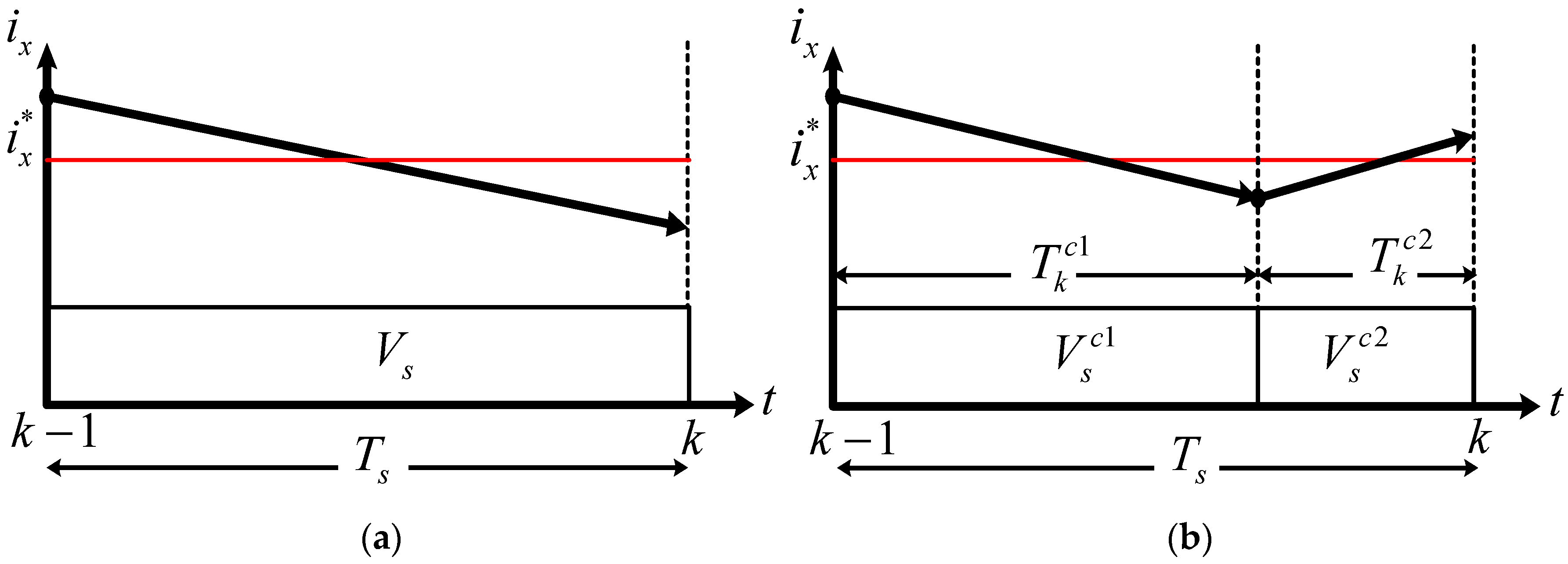
In a sampling period, the applications of two successive voltage vectors are allowed to operate together with two optimal duty ratios while achieving the current predictions. It is worth noting that these optimized duty ratios are calculated online.

2

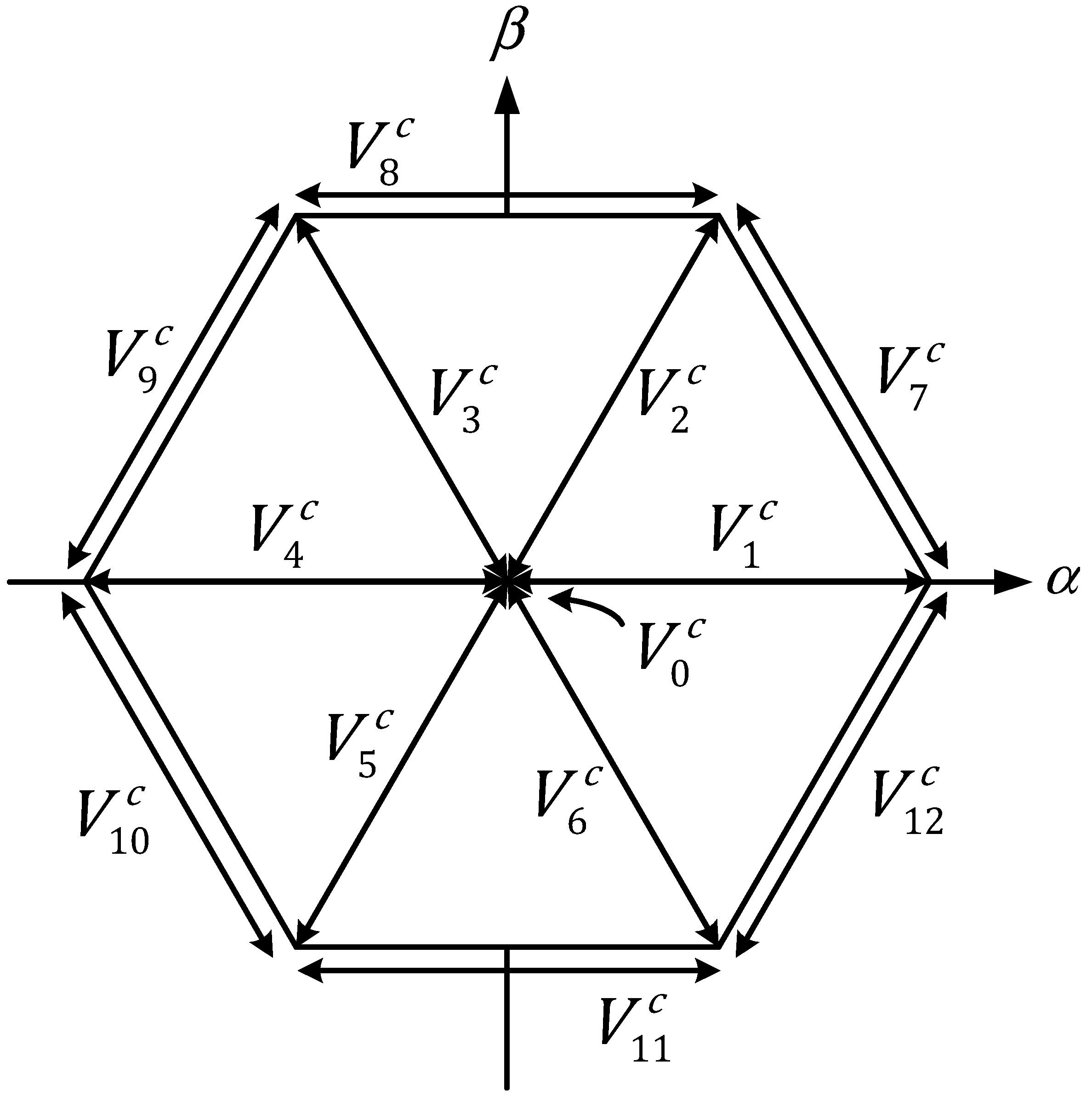
More candidate switching modes are obtained via the linear combinations of two voltage vectors, increased from the typical seven switching modes described in [20] to thirteen when using the proposed control strategy, thus enhancing control efficiency while retaining the simplicity of the algorithm.

3

The duty ratio is taken as a variable; hence, it is incorporated into the cost function and optimized.

4

This is the first implementation of such an MMPCC on the IPMSM drive system.

The rest of the article is organized as follows. An MPC-based current control is presented in Section 2, followed by Section 3, which discusses the proposed scheme in detail. The experimental platform, setup and results are provided in Section 4, and finally, the conclusion is given in Section 5.

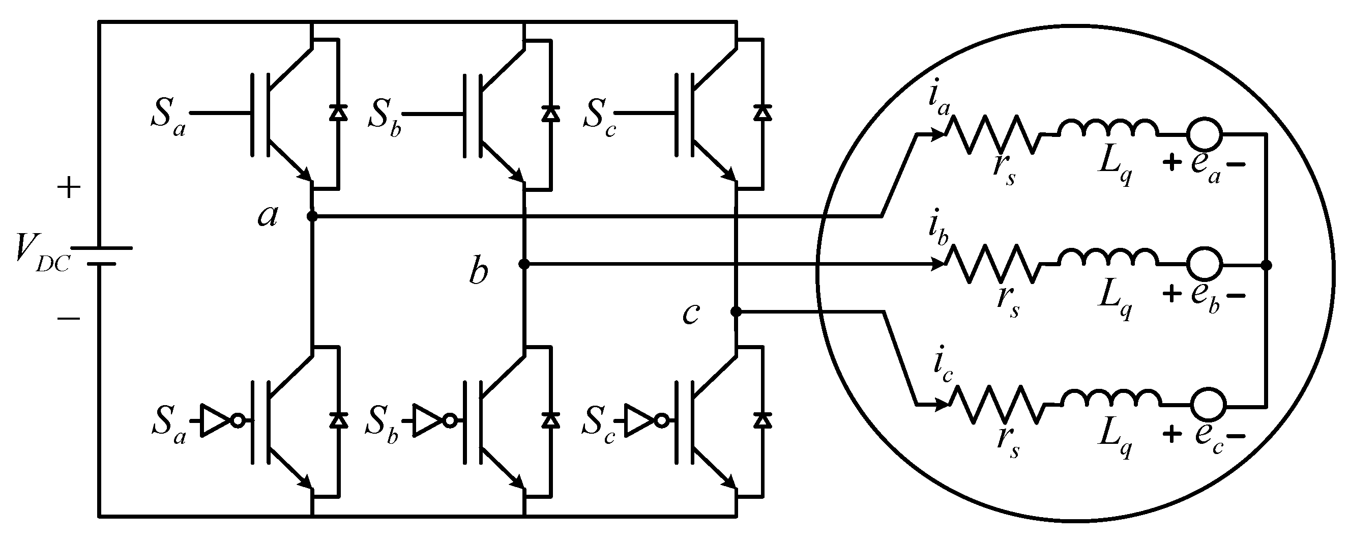
2. Current Control Prediction Based on Conventional MPC

The algorithm of a typical model predictive current control (MPCC) is primarily based on the discretization of the associated mathematical model to predict the currents. Based on the criterion of cost function minimization [3], data are collected from the motor operation and then utilized so as to identify the optimal actuation.

The schematic diagram of a typical three-phase six-switch inverter-fed interior permanent-magnet synchronous motor is shown in Figure 1. The voltage source inverter contains six switches controlled by signals S_a, S_b, and S_c. Other components include: the dc-link voltage, V_DC; the stator voltages, v_a, v_b, v_c; the stator currents, i_a, i_b, i_c; the extended back EMF, e_a, e_b, e_c; the stator resistance, r_s; and the q-axis inductance, L_q.

2.1. Mathematical Model of IPMSM

The stator voltage equation of IPMSM expressed in the three-phase stationary reference frame is shown in Equation (1). However, due to its highly complex characteristics, the differential equation of electrical dynamics is given below under an ideal condition wherein the current loss, the hysteresis loss, and the magnetic saturations are assumed to be negligible [28].

$$v_x=r_s{i}_x+L_q\frac{d}{dt}{\psi }_z , x\in \left\{a, b, c\right\}$$

(1)

where $\frac{d}{dt}$ refers to the differential operator, $i_x$ stands for the phase-wise stator current, and ${\psi }_z$ represents the phase-wise stator flux linkage produced by the self-linked flux of stator currents and rotor magnets. The cross-coupling effects between the inductances brought by ${\psi }_z$ make the IPMSM a highly nonlinear system, and hence complex in nature. The following method can be employed to simplify the above expression, leading to a two-axis model [20].

$$\left[\begin{array}{c}{\psi }_a\\ {\psi }_b\\ {\psi }_c\end{array}\right]=\left[\begin{array}{cc}\begin{array}{cc}{L}_{aa}& L_{ab}\end{array}& L_{ac}\\ \begin{array}{c}\begin{array}{cc}{L}_{ba}& L_{bb}\end{array}\\ \begin{array}{cc}{L}_{ca}& L_{cb}\end{array}\end{array}& \begin{array}{c}{L}_{bc}\\ L_{cc}\end{array}\end{array}\right]+{\psi }_m\left[\begin{array}{c}\cos {\theta }_{re}\\ \cos ({\theta }_{re}-\frac{2\pi }{3})\\ \cos ({\theta }_{re}+\frac{2\pi }{3})\end{array}\right]$$

(2)

where ${\psi }_m$ is the rotor flux linkage and ${\theta }_{re}$ is the rotor angle of the motor. The effect of cross-coupling in the two-axis model is considered to be the self-inductances represented by $L_{aa}$, $L_{bb}$, and $L_{cc}$, and the mutual inductances by $L_{ab}$, $L_{ba}$, $L_{bc}$, $L_{cb}$, $L_{ac}$ and $L_{ca}$. The respective values can be obtained through

$$\left[\begin{array}{c}{L}_{aa}\\ L_{bb}\\ L_{cc}\end{array}\right]=\left[\begin{array}{c}{L}_{ls}\\ L_{ls}\\ L_{ls}\end{array}\right]+\left[\begin{array}{c}{L}_A\\ L_A\\ L_A\end{array}\right]-L_B\left[\begin{array}{c}\cos (2{\theta }_{re})\\ \cos (2{\theta }_{re}+\frac{2\pi }{3})\\ \cos (2{\theta }_{re}-\frac{2\pi }{3})\end{array}\right]$$

(3)

$$\left[\begin{array}{c}{L}_{ab}\\ L_{bc}\\ L_{ca}\end{array}\right]=\left[\begin{array}{c}{L}_{ba}\\ L_{cb}\\ L_{ac}\end{array}\right]=-\frac{1}{2}\left[\begin{array}{c}{L}_A\\ L_A\\ L_A\end{array}\right]-L_B\left[\begin{array}{c}\cos (2{\theta }_{re}-\frac{2\pi }{3})\\ \cos (2{\theta }_{re})\\ \cos (2{\theta }_{re}+\frac{2\pi }{3})\end{array}\right]$$

(4)

The variables $L_A$, $L_B,$ and $L_{ls}$ represent the DC component of the inductance, the magnitude of the cosine function of the inductance, and the coil leakage inductance, respectively. Given Equations (2)–(4), Equation (1) can be expanded to yield the following three-phase stator voltage expressions [20]:

$$\begin{gathered} v_a=r_s{i}_a+\frac{d}{dt}[{\lambda }_m\cos {\theta }_{re}+\left(L_{ls}+L_A-L_B\cos (2{\theta }_{re}\right))i_a+(-\frac{1}{2}{L}_A-L_B\cos (2{\theta }_{re}-\frac{2\pi }{3}))i_b \\ +\left(-\frac{1}{2}{L}_A-L_B\cos (2{\theta }_{re}+\frac{2\pi }{3})\right)i_c] \end{gathered}$$

(5)

$$\begin{gathered} v_b=r_s{i}_b+\frac{d}{dt}[{\lambda }_m\cos \left({\theta }_{re}-\frac{2\pi }{3}\right)+(-\frac{1}{2}{L}_A-L_B\cos (2{\theta }_{re}-\frac{2\pi }{3}))i_a \\ +\left(L_{ls}+L_A-L_B\cos (2{\theta }_{re}+\frac{2\pi }{3}\right)i_b+\left(-\frac{1}{2}{L}_A-L_B\cos (2{\theta }_{re})\right)i_c] \end{gathered}$$

(6)

$$\begin{gathered} v_c=r_s{i}_c+\frac{d}{dt}[{\lambda }_m\cos \left({\theta }_{re}+\frac{2\pi }{3}\right)+(-\frac{1}{2}{L}_A-L_B\cos (2{\theta }_{re}+\frac{2\pi }{3}))i_a +\left(-\frac{1}{2}{L}_A- \\ {L}_B\cos (2{\theta }_{re})\right)i_b+\left(L_{ls}+L_A-L_B\cos (2{\theta }_{re}-\frac{2\pi }{3}\right)i_b] \end{gathered}$$

(7)

The transformation of motor inductances between stator and rotor can be simplified through the equivalent quadrature value of inductance in the two-axis model. The q-axis inductance, $L_q$, is taken to be constant in this article and is defined as in [21].

$$L_q=L_{ls}+\frac{3\left(L_A+L_B\right)}{2}$$

(8)

Given the definition as of Equation (8), the three-phase stator voltage can be simplified as [21]:

$$v_z=r_s{i}_z+L_q\frac{d}{dt}{i}_z+e_z, z\in \left\{a,b,c\right\},$$

(9)

where $e_z$ is the phase-wise extended back EMF. Moreover, the $a-b-c$ three-phase reference frame of IPMSM is not orthogonal in nature and the asymmetrical components are difficult to control. It is impossible to vary one axis without affecting the others. To circumvent these constraints and simplify the analysis, the $\alpha -\beta$ transformation is employed, which is widely adopted. This will reduce the projections of the phase quantities into the two-axis model reference frame. Following the $\alpha -\beta$ transformation, the counterpart of Equation (9) can be written as:

$$v_{\alpha }=r_s{i}_{\alpha }+L_q\frac{d}{dt}{i}_{\alpha }+e_{\alpha }$$

(10)

$$v_{\beta }=r_s{i}_{\beta }+L_q\frac{d}{dt}{i}_{\beta }+e_{\beta }$$

(11)

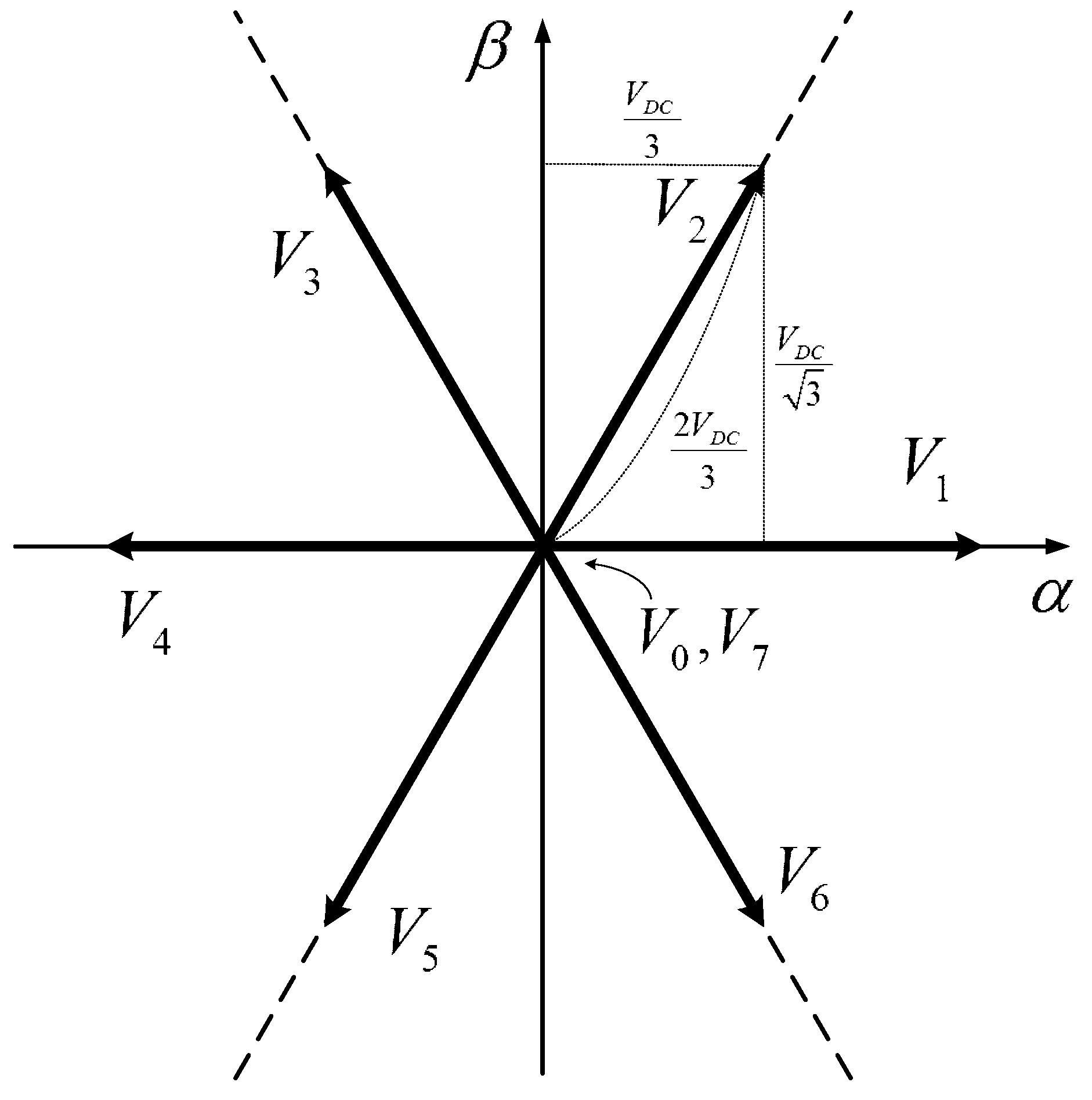
2.2. Optimal Voltage Vector Selection

The field-oriented control (FOC) is commonly used in motor drive systems powered by three-phase six-switch voltage source inverters (VSIs). Given the six-switch topology, a VSI can generate eight basic voltage vectors in general. Together with linear controllers [3], the FOC provides the three-phase voltages required for the IPMSM drive systems. Unlike FOC, the MPC determines the future voltage vector based on the predefined selection of switching states. Ideally, the optimal selection of the future voltage vector should yield the lowest cost function value.

The eight switching voltage vectors are shown in Figure 2, containing two zero-voltage vectors, $V_0$ and $V_7$, and six non-zero or the active voltage vectors, $V_1$, $V_2$, $V_3$, $V_4$, $V_5$, and $V_6$. Associated with them are the switching states, $S_0$–$S_7$. Given in

Table 1. Three-phase six-switch VSI switching state table.

Switching State		Three-Phase Output Voltage			$\mathit{\alpha }-\mathit{\beta }\mathbf{Equivalent}\mathbf{Voltage}$		Voltage Vector
$S$	$\left(S_a{S}_b{S}_c\right)$	$v_a$	$v_b$	$v_c$	$v_{\alpha }$	$v_{\beta }$	$V_0$
$S_0$	$\left(000\right)$	0	0	0	0	0	$V_0$
$S_1$	$\left(001\right)$	$-V_{DC}/3$	$-V_{DC}/3$	$2V_{DC}/3$	$-V_{DC}/3$	$-\sqrt{3}{V}_{DC}/3$	$V_1$
$S_2$	$\left(010\right)$	$-V_{DC}/3$	$2V_{DC}/3$	$-V_{DC}/3$	$-V_{DC}/3$	$\sqrt{3}{V}_{DC}/3$	$V_2$
$S_3$	$\left(011\right)$	$-2V_{DC}/3$	$V_{DC}/3$	$V_{DC}/3$	$-2V_{DC}/3$	0	$V_3$
$S_4$	$\left(100\right)$	$2V_{DC}/3$	$-V_{DC}/3$	$-V_{DC}/3$	$2V_{DC}/3$	0	$V_4$
$S_5$	$\left(101\right)$	$V_{DC}/3$	$-2V_{DC}/3$	$V_{DC}/3$	$V_{DC}/3$	$-\sqrt{3}{V}_{DC}/3$	$V_5$
$S_6$	$\left(110\right)$	$V_{DC}/3$	$V_{DC}/3$	$-2V_{DC}/3$	$V_{DC}/3$	$\sqrt{3}{V}_{DC}/3$	$V_6$
$S_7$	$\left(111\right)$	0	0	0	0	0	$V_7$

are the details of the relationships between the switching states, the three-phase voltage outputs, the equivalent stator voltages, and the switching function.

It can also be observed from Table 1 that the output voltages of $V_0$ and $V_7$ are zero, and they are, in theory, considered identical. This reduces the number of total switching states from eight to seven, and they are $S_0$, $S_1$, $S_2$, $S_3$, $S_4$, $S_5$, and $S_6$.

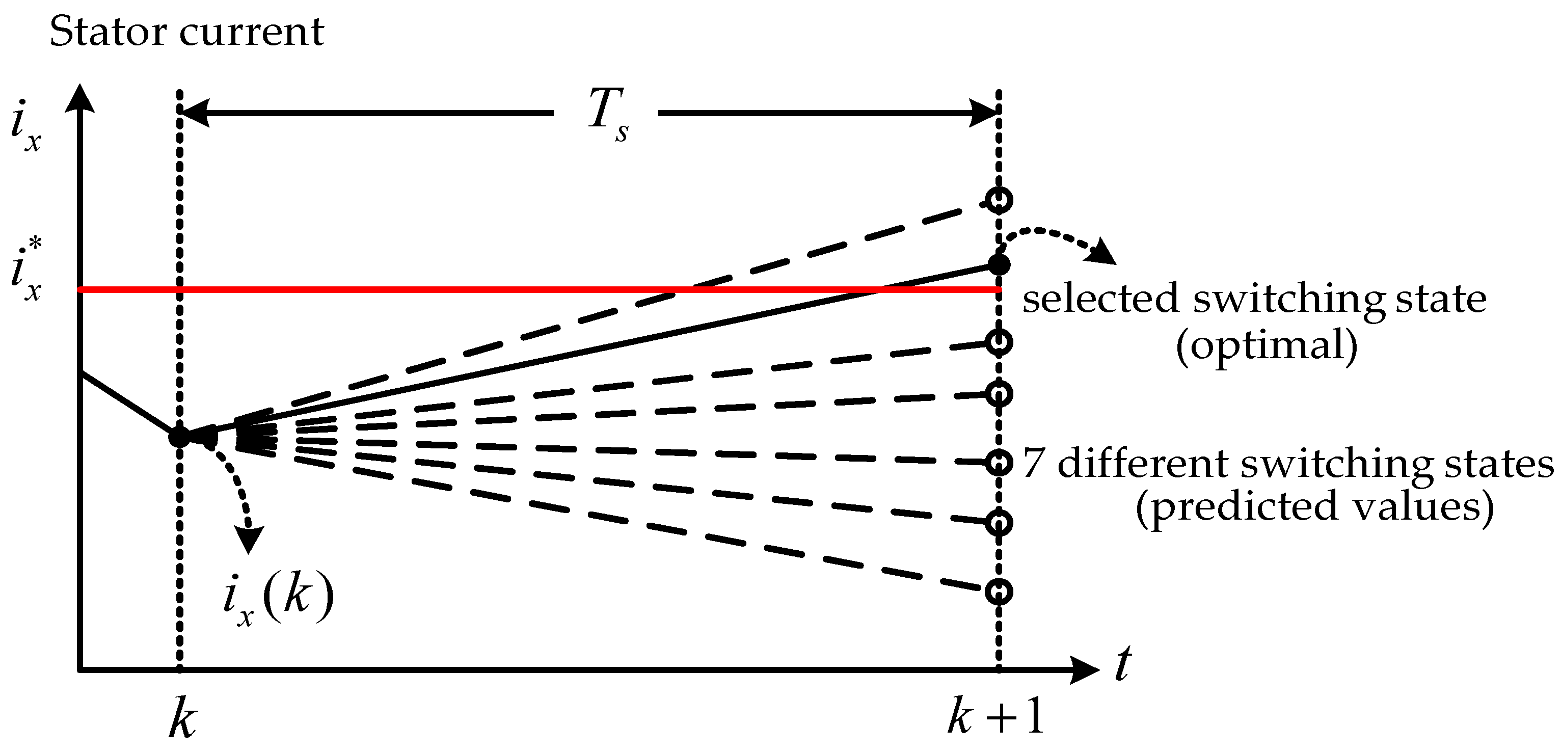
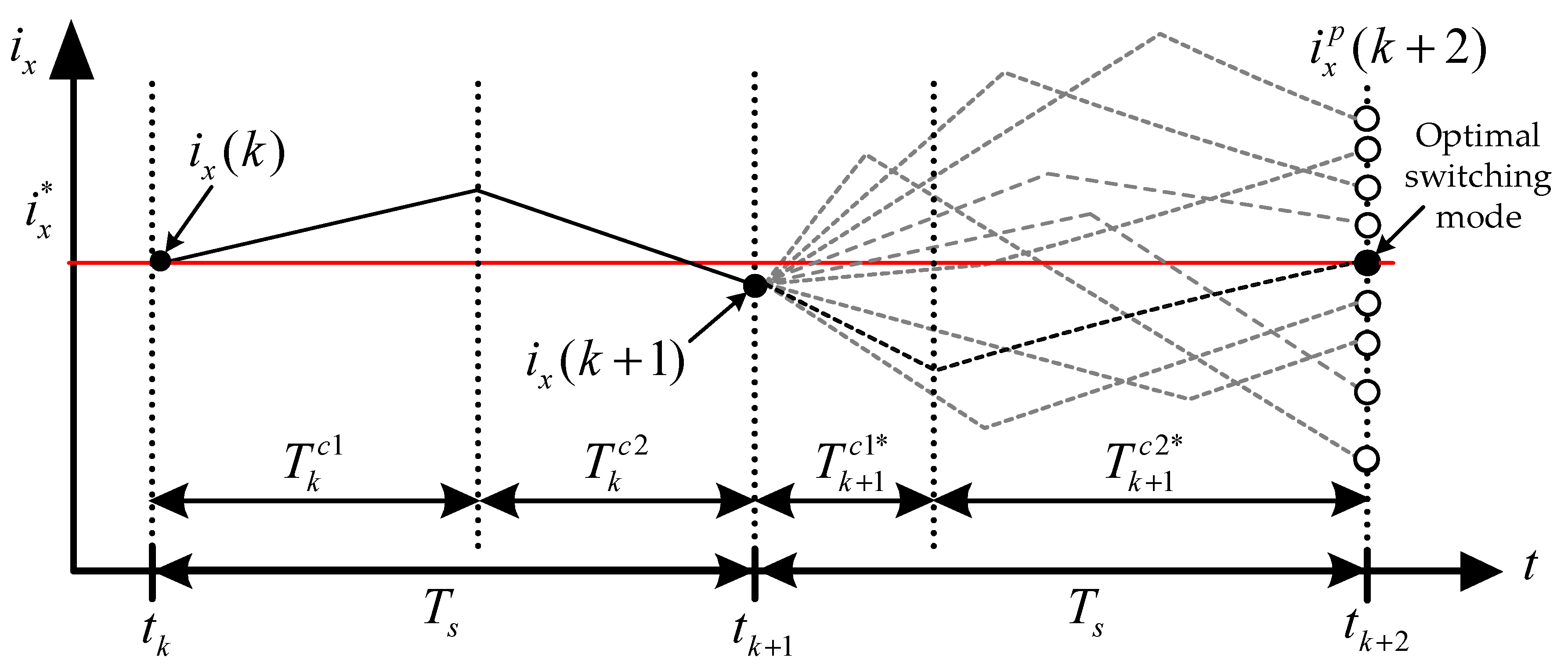
2.3. Current Prediction Strategy

Compared to FOC, the MPC possesses certain flexibility and extensibility features. In addition, thanks to the performance advancement of modern microcontrollers, the MPC is able to predict the stator currents under all candidate switching modes within a sampling period. For the MPC to be realized and its operation carried out on a microcontroller, all continuous variables are approximated by discretized forms. As an example, the time derivative of current is approximated by:

$$\frac{d}{dt}{i}_x\approx \frac{i_x\left(k\right)-i_x\left(k-1\right)}{T_s},$$

(12)

assuming the sampling period $T_s$ is short enough. Given the above condition, Equations (10) and (11) can be expressed in an equivalent discretized form as:

$$v_x\left(k\right)=r_s{i}_x\left(k\right)+L_q\frac{i_x\left(k\right)-i_x\left(k-1\right)}{T_s}+e_x\left(k\right),$$

(13)

where $x\in \left\{\alpha ,\beta \right\}$ and $k$ stands for the $\left(k\right)\mathrm{th}$ period. With time delay compensation taken into account [29], the above equations can be rearranged to yield the $\left(k+1\right)\mathrm{th}$ and $\left(k+2\right)\mathrm{th}$ predicted currents as follows:

$$i_x^{\mathrm{p}}\left(k+1\right)=\frac{1}{(r_s{T}_s+L_q)}\left(L_q{i}_x^{\mathrm{P}}\left(k\right)+T_s{v}_x\left(k\right)-T_s\widehat{e_x}\left(k\right)\right)$$

(14)

$$i_x^{\mathrm{p}}\left(k+2\right)=\frac{1}{(r_s{T}_s+L_q)}\left(L_q{i}_x^{\mathrm{P}}\left(k+1\right)+T_s{v}_x\left(k+1\right)-T_s\widehat{e_x}\left(k+1\right)\right)$$

(15)

where the superscripts “$\mathrm{p}$” and “$^$” represent the predicted current and estimated extended back-EMF, respectively. To circumvent the difficulty of getting the value of $\widehat{e_x}\left(k+1\right)$, one may again assume that the sampling period is sufficiently short and use:

$$\widehat{e_x}\left(k+1\right)\approx \widehat{e_x}\left(k\right)=v_x\left(k\right)+\frac{L_q}{T_s}{i}_x\left(k-1\right)-\frac{r_s{T}_s+L_q}{T_s}{i}_x\left(k\right)$$

(16)

Given Equation (15), Equation (16) can be rewritten as

$$i_x^{\mathrm{p}}\left(k+2\right)=K_1{i}_x\left(k-1\right)+K_2{i}_x\left(k\right)+K_3{v}_x\left(k-1\right)+K_4{v}_x\left(k\right)+K_5{v}_x\left(k+1\right)$$

(17)

where $K_1=-L_q\left(2L_q+r_s{T}_s\right)/K_6$, $K_2=\left(3L_q^2+3L_q{r}_s{T}_s+r_s^2{T}_s^2\right)/K_6$, $K_3=\left(-r_s{T}_s^2-2L_q{T}_s\right)/K_6$, $K_4=L_q{T}_s/K_6$, $K_5=\left(r_s{T}_s^2+L_q{T}_s\right)/K_6$, and $K_6={(L_q+r_s{T}_s)}^2$. The voltage $v_x\left(k+1\right)$, appearing in Equation (17), can be found from Table 1. To achieve optimal switching, the predicted current should be as close as possible to the current command. To that end, a cost function $g$ is defined as follows:

$$g={(i_{\alpha }^{*}\left(k\right)-i_{\alpha }^{\mathrm{p}}\left(k+2\right))}^2+{(i_{\beta }^{*}\left(k\right)-i_{\beta }^{\mathrm{p}}\left(k+2\right))}^2$$

(18)

where the superscript “*” refers the command or, interchangeably, the reference. The switching state yielding the minimum cost value will then be selected and applied in the next sampling period. Details of the method are shown in the schematic diagram of Figure 3.

3. Proposed Modulated Model Predictive Current Control

Conventional MPC typically applies a single voltage vector in each sampling period, as shown in Figure 4a, and produces large current ripples when it is applied to the IPMSM drive system. To improve this situation, a modulated model predictive current control (MMPCC) is proposed, as shown in Figure 4b. The basic idea behind this is to make the voltage application time adaptive and optimized by incorporating the mechanism of vector modulation into the MPC. It can be seen from Figure 4b that two voltage vectors $V_s^{c1}$ and $V_s^{c2}$ are applied successively for current prediction in a sampling period, with durations $T_k^{c1}$ and $T_k^{c2}$, respectively. One gains apparent benefits by using two modulated voltage vectors whose application durations are adapted and optimized online. This is a very important and appealing feature, in contrast to conventional MPCCs without modulation, whose voltage application time is fixed. To reduce the difficulty of implementation and the computation time, thirteen switching modes were considered for current predictions.

3.1. Design of Adaptive Duty Ratio Modulation

Taking the (k)th sampling period, for instance, the two durations are represented by $T_k^{c1}$ and $T_k^{c2}$, respectively, for the two consecutive voltage vectors, $V_s^{c1}$ and $V_s^{c2}$. The superscript $“c”$ refers to the resulting synthesized value of modulation. Accordingly, the sampling period $T_s$ can be expressed as:

$$T_k^{c1}+T_k^{c2}=T_s$$

(19)

The two duty ratios corresponding to $V_s^{c1}$ and $V_s^{c2}$ are designated $D_k^{c1}$ and $D_k^{c1}$, respectively, and are defined as:

$$D_k^{c1}=T_k^{c1}/T_s$$

(20)

$$D_k^{c2}=T_k^{c2}/T_s$$

(21)

As a result of Equations (20) and (21), the sum of the two duty ratios $D_k^{c1}$ and $D_k^{c1}$ satisfies the following identity:

$$D_k^{c1}+D_k^{c2}=1$$

(22)

Further details of Equation (19) are discussed in Section 3.3. Due to practical reasons and the limitations of the motor drive system, oftentimes, lower and upper limits are imposed on the duty ratios $D_k^{c1}$ and $D_k^{c2}$. That is, $0.2T_s<T_k^{c1}\le 0.8T_s$ and $T_k^{c2}=T_s-T_k^{c1}$.

3.2. Synthesized Voltage Vectors and Current Prediction

To implement the proposed method and reduce the computational complexity, thirteen synthesized voltage vectors, labeled as $V_{01}^c$–$V_{12}^c$, are used, each of which is synthesized by two different or identical voltage vectors. As shown in Figure 5, thirteen synthesized voltage vectors are projected onto the α–β plane, including a zero-voltage vector $V_0^c$ at the center, six co-adjacent non-zero voltage vectors $V_1^c–V_6^c$, and six non-zero voltage vectors across the edges $V_7^c–V_{12}^c$. As can be seen from Figure 4b, the application times $T_k^{c1}$ and $T_k^{c2}$ are adaptive, meaning that the two duty ratios $D_k^{c1}$ and $D_k^{c2}$ are adaptive. As such, the value of the (k)th synthesized voltage $v_x^c\left(k\right)$ can be expressed as

$$v_x^c\left(k\right)=D_k^{c1}{V}_x^{c1}\left(k\right)+D_k^{c2}{V}_x^{c2}\left(k\right), x\in \left\{\alpha ,\beta \right\},$$

(23)

where $V_x^{c1}\left(k\right)$ and $V_x^{c2}\left(k\right)$ are the stator voltages corresponding to the two consecutive voltage vectors applied in the $\left(k\right)\mathrm{th}$ sampling period. Equation (22) implies:

$$D_k^{c2}=1-D_k^{c1}$$

(24)

Next, substitution of (24) into (23) yields the following equation:

$$v_x^c\left(k\right)=D_k^{c1}{V}_x^{c1}\left(k\right)+\left(1-D_k^{c1}\right)V_x^{c2}\left(k\right)$$

(25)

Equation (25) can be utilized to obtain the $\left(k-1\right)\mathrm{th}$ and $\left(k+1\right)\mathrm{th}$ synthesized voltage vectors $v_x^c\left(k-1\right)$ and $v_x^c\left(k+1\right)$ as follows:

$$v_x^c\left(k-1\right)=D_{k-1}^{c1}{V}_x^{c1}\left(k-1\right)+\left(1-D_{k-1}^{c1}\right)V_x^{c2}\left(k-1\right)$$

(26)

$$v_x^c\left(k+1\right)=D_{k+1}^{c1}{V}_x^{c1}\left(k+1\right)+\left(1-D_{k+1}^{c1}\right)V_x^{c2}\left(k+1\right)$$

(27)

Please note that the voltage vectors $V_0~V_7$ correspond to the switching states $S_0–S_7$, as shown in Table 1. The thirteen synthesized voltage vectors and the two applied switching states are listed in

Table 2. Synthesized voltage vectors and switching states.

$\mathbf{Synthesized}\mathbf{Voltage}\mathbf{Vector}\left({\mathit{V}}_{\mathit{k}}^{\mathit{c}}\right)$	Linear Combination	$\mathbf{Two}\mathbf{Applied}\mathbf{Switching}\mathbf{State}\left({\mathit{S}}_{\mathit{k}}^{\mathit{c}}\right)$
		First	Second
$V_0^c$	$(T_k^{c1}{V}_0+T_k^{c2}{V}_0)/T_s$	$S_0\left(000\right)$	$S_0\left(000\right)$
$V_1^c$	$(T_k^{c1}{V}_1+T_k^{c2}{V}_0)/T_s$	$S_4\left(100\right)$	$S_0\left(000\right)$
$V_2^c$	$(T_k^{c1}{V}_2+T_k^{c2}{V}_0)/T_s$	$S_6\left(110\right)$	$S_0\left(000\right)$
$V_3^c$	$(T_k^{c1}{V}_3+T_k^{c2}{V}_0)/T_s$	$S_2\left(010\right)$	$S_0\left(000\right)$
$V_4^c$	$(T_k^{c1}{V}_4+T_k^{c2}{V}_0)/T_s$	$S_3\left(011\right)$	$S_0\left(000\right)$
$V_5^c$	$(T_k^{c1}{V}_5+T_k^{c2}{V}_0)/T_s$	$S_1\left(001\right)$	$S_0\left(000\right)$
$V_6^c$	$(T_k^{c1}{V}_6+T_k^{c2}{V}_0)/T_s$	$S_5\left(101\right)$	$S_0\left(000\right)$
$V_7^c$	$(T_k^{c1}{V}_1+T_k^{c2}{V}_2)/T_s$	$S_4\left(100\right)$	$S_6\left(110\right)$
$V_8^c$	$(T_k^{c1}{V}_2+T_k^{c2}{V}_3)/T_s$	$S_6\left(110\right)$	$S_2\left(010\right)$
$V_9^c$	$(T_k^{c1}{V}_3+T_k^{c2}{V}_4)/T_s$	$S_2\left(010\right)$	$S_3\left(011\right)$
$V_{10}^c$	$(T_k^{c1}{V}_4+T_k^{c2}{V}_5)/T_s$	$S_3\left(011\right)$	$S_1\left(001\right)$
$V_{11}^c$	$(T_k^{c1}{V}_5+T_k^{c2}{V}_6)/T_s$	$S_1\left(001\right)$	$S_5\left(101\right)$
$V_{12}^c$	$(T_k^{c1}{V}_6+T_k^{c2}{V}_1)/T_s$	$S_5\left(101\right)$	$S_4\left(100\right)$

.

Given Table 1, it is not difficult to find $V_x^{c1}\left(k-1\right)$, $V_x^{c2}\left(k-1\right)$, $V_x^{c1}\left(k\right)$, $V_x^{c2}\left(k\right)$, $V_x^{c1}\left(k+1\right)$, and $V_x^{c2}\left(k+1\right) \in \left\{-\frac{2V_{DC}}{3},-\frac{\sqrt{3}{V}_{DC}}{3},-\frac{V_{DC}}{3}, 0, \frac{V_{DC}}{3}, \frac{\sqrt{3}{V}_{DC}}{3}, \frac{2V_{DC}}{3}\right\}$, as of (23)–(27). Next, the three variables $v_x\left(k-1\right)$, $v_x\left(k\right)$, and $v_x\left(k+1\right)$ are replaced by $v_x^c\left(k-1\right)$, $v_x^c\left(k\right)$, and $v_x^c\left(k+1\right)$, respectively, to provide the predicted $\left(k+2\right)\mathrm{th}$ $\alpha$-axis and β-axis currents as:

$$i_{\alpha }^{\mathrm{P}}\left(k+2\right)=K_1{i}_{\alpha }\left(k-1\right)+K_2{i}_{\alpha }\left(k\right)+K_3{v}_{\alpha }^c\left(k-1\right)+K_4{v}_{\alpha }^c\left(k\right)+K_5{v}_{\alpha }^c\left(k+1\right)$$

(28)

$$i_{\beta }^{\mathrm{P}}\left(k+2\right)=K_1{i}_{\beta }\left(k-1\right)+K_2{i}_{\beta }\left(k\right)+K_3{v}_{\beta }^c\left(k-1\right)+K_4{v}_{\beta }^c\left(k\right)+K_5{v}_{\beta }^c\left(k+1\right)$$

(29)

where the superscript “p” stands for prediction; $i_{\alpha }\left(k-1\right)$ and $i_{\alpha }\left(k\right)$ are the $\alpha$-axis currents measured at the $\left(k-1\right)\mathrm{th}$ and $\left(k\right)\mathrm{th}$ samplings, respectively; $i_{\beta }\left(k-1\right)$ and $i_{\beta }\left(k\right)$ are the $\beta$-axis currents measured at the $\left(k-1\right)\mathrm{th}$ and $\left(k\right)\mathrm{th}$ samplings, respectively; $v_{\alpha }^c\left(k-1\right)$, $v_{\alpha }^c\left(k\right)$, and $v_{\alpha }^c\left(k+1\right)$ are the $\alpha$-axis synthesized voltage vectors at the $\left(k-1\right)\mathrm{th}$, $\left(k\right)\mathrm{th}$ and $\left(k+1\right)\mathrm{th}$ samplings, respectively; $v_{\beta }^c\left(k-1\right)$, $v_{\beta }^c\left(k\right)$, and $v_{\beta }^c\left(k+1\right)$ are the $\beta$-axis synthesized voltage vectors at the $\left(k-1\right)\mathrm{th}$, $\left(k\right)\mathrm{th}$ and $\left(k+1\right)\mathrm{th}$ samplings, respectively.

3.3. Cost Function Design and Optimized Modulation Ratios

The proposed MMPCC retains an important criterion of model predictive control—the cost function design. In reference to Equations (11) and (15), a new cost function G applicable to the MMPCC is defined as:

$$G={(i_{\alpha }^{*}\left(k\right)-i_{\alpha }^{\mathrm{P}}\left(k+2\right))}^2+{(i_{\beta }^{*}\left(k\right)-i_{\beta }^{\mathrm{P}}\left(k+2\right))}^2$$

(30)

Using Equations (25)–(27) and substituting (28) and (29) into (30), one can rewrite (30) as:

$$G={(K_{\alpha 1}+D_{k+1}^{c1}{K}_{\alpha 2})}^2+{(K_{\beta 1}+D_{k+1}^{c1}{K}_{\beta 2})}^2$$

(31)

where $K_{\alpha 1}=i_{\alpha }^{*}\left(k\right)-K_1{i}_{\alpha }\left(k-1\right)-K_2{i}_{\alpha }\left(k\right)-K_3{v}_{\alpha }^c\left(k-1\right)-K_4{v}_{\alpha }^c\left(k\right)-K_5{V}_{\alpha }^{c2}\left(k+1\right)$, $K_{\alpha 2}=K_5\left(V_{\alpha }^{c2}\left(k+1\right)-V_{\alpha }^{c1}\left(k+1\right)\right)$, $K_{\beta 1}=i_{\beta }^{*}\left(k\right)-K_1{i}_{\beta }\left(k-1\right)-K_2{i}_{\beta }\left(k\right)-K_3{v}_{\beta }^c\left(k-1\right)-K_4{v}_{\beta }^c\left(k\right)-K_5{V}_{\beta }^{c2}\left(k+1\right)$, $K_{\beta 2}=K_5\left(V_{\beta }^{c2}\left(k+1\right)-V_{\beta }^{c1}\left(k+1\right)\right)$. Ideally, the optimal switching mode is that which yields the minimum cost value. However, the above calculation cannot be implemented if the duty ratio $D_{k+1}^{c1}$ is unknown. To proceed, the optimal duty ratio $D_{k+1}^{c1}$ needs to be determined first. Assuming a partial derivative of the cost function $G$ with respect to the duty ratio $D_{k+1}^{c1}$ exists, one can easily obtain the following expression:

$$\frac{\partial G}{\partial D_{k+1}^{c1}}=2K_{\alpha 2}\left(K_{\alpha 1}+D_{k+1}^{c1}{K}_{\alpha 2}\right)+2K_{\beta 2}\left(K_{\beta 1}+D_{k+1}^{c1}{K}_{\beta 2}\right)$$

(32)

Let $\frac{\partial G}{\partial D_{k+1}^{c1}}=0$, one then gets the following optimal duty ratio, which is denoted as $D_{k+1}^{c1*}$:

$$D_{k+1}^{c1*}=\left(-K_{\alpha 1}{K}_{\alpha 2}-K_{\beta 1}{K}_{\beta 2}\right)/\left(K_{\alpha 2}^2+K_{\beta 2}^2\right)$$

(33)

With the duty ratio $D_{k+1}^{c1}$ in Equation (31) replaced by $D_{k+1}^{c1*}$, the cost function now becomes:

$$G^{*}={(K_{\alpha 1}+D_{k+1}^{c1*}{K}_{\alpha 2})}^2+{(K_{\beta 1}+D_{k+1}^{c1*}{K}_{\beta 2})}^2$$

(34)

It is worth mentioning that different synthesized voltages yield different optimal duty ratios. As such, the thirteen optimal duty ratios corresponding to the thirteen switching modes need to be calculated online first. These optimal values are then substituted back into the cost function for minimization. Given Equation (34), thirteen cost values can be obtained by means of the thirteen synthesized voltage vectors listed in Table 2. The vector is considered to be optimal so long as it gives the minimum cost value. Given Table 2, the two switching states can be found through table-lookup and applied for durations $T_{k+1}^{c1*}$ and $T_{k+1}^{c2*}$, respectively, in the next sampling period. Specifically, the optimal durations $T_{k+1}^{c1*}$ and $T_{k+1}^{c2*}$ are defined as

$$T_{k+1}^{c1*}=D_{k+1}^{c1*}{T}_s$$

(35)

$$T_{k+1}^{c2*}=1-T_{k+1}^{c1*}$$

(36)

The fundamental principle of the proposed MMPCC is illustrated in detail by Figure 6. The novel design of the cost function calculation in Equation (34) allows thirteen unique predicted values of stator currents, of which the cost value with optimal durations, as described in Equations (35) and (36), will be applied in the next sampling period. As a result, the optimal switching mode will naturally lead to the smallest current error in the (k + 2)th sampling period.

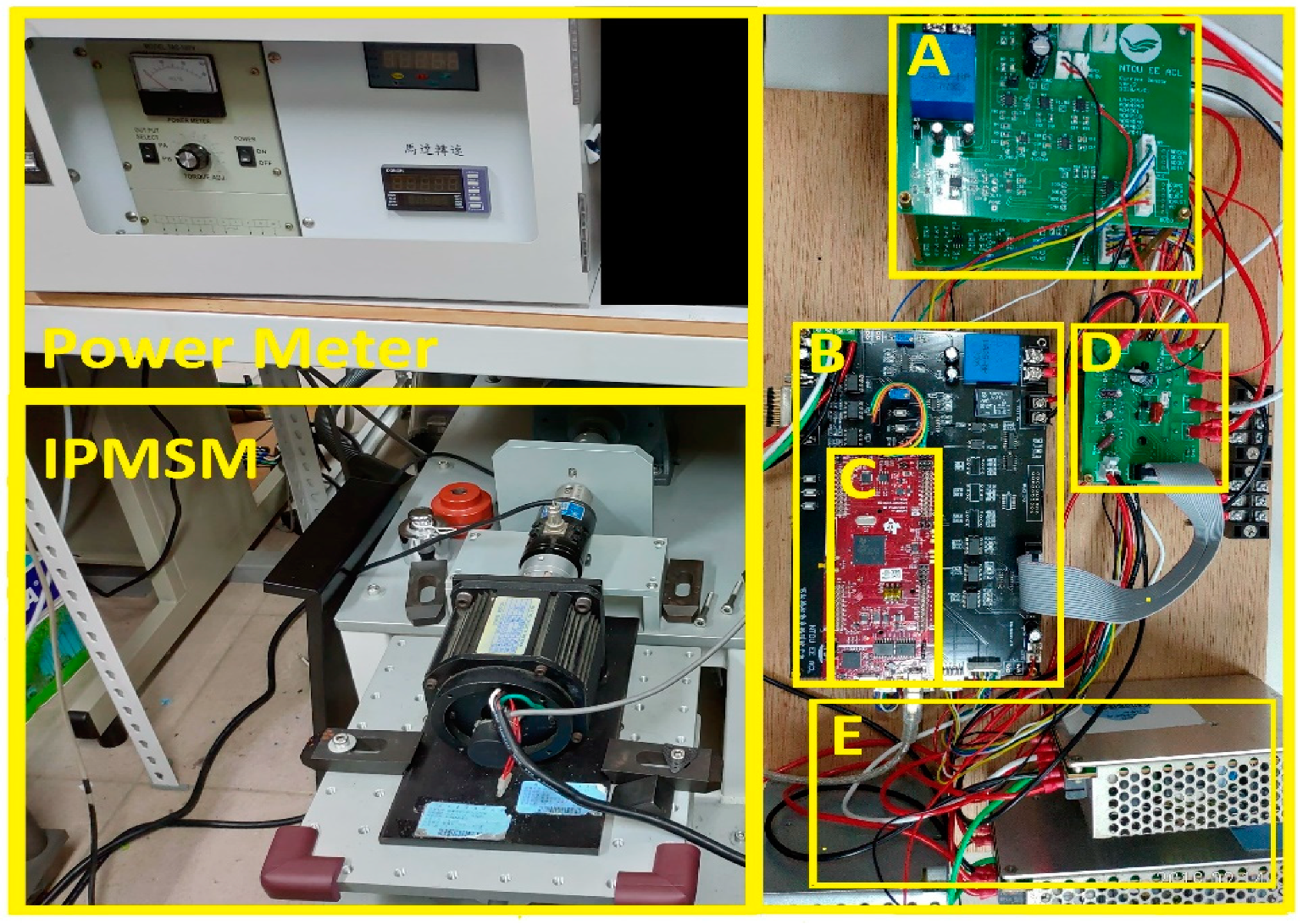
4. Experimental Test Stand and Results

To validate the proposed MMPCC and evaluate its effectiveness, several experiments were carried out through the microcontroller TMS320F28379D of Texas Instruments (Dallas, TX, United States), and performance comparisons were made against the MPCC without modulation. The hardware drive circuit is shown in Figure 7, containing a power meter, an IPMSM, and including several other important components: Part A is composed of two current detection boards used to measure the a and b phase currents, respectively, and each board contains a current sensor of LA25-NP type by LEM Co. Ltd. (Plan-les-Ouates, Geneva, Switzerland), a current/voltage conversion circuit, and a 16-bit A/D converter. The bandwidth of the LA25-NP is 150 kHz, with ±25 A as its range. Part B includes an overcurrent protection circuit, an encoder circuit, and several HCPL2631 optocouplers made by Fairchild Semiconductor. The overcurrent protection circuit protects against excessive current, disabling the system instantaneously to avoid damage. Part C is the TMS320F28379D dual-core microcontroller made by Texas Instruments. The microcontroller consists of two sets of TMS320C28x 32-bit CPUs capable of high-speed data processing at up to 200 MHz. Part D consists of a low switching dissipation insulated gate bipolar transistors (IGBT) power module inverter (SCM1246MF) made by Sanken Electric Co. Ltd. (Niiza-shi, Saitama-ken, Japan), with an output breakdown voltage of 600 V and output current of 30 A. The inverter includes six sets of IGBTs and freewheeling diodes, and three sets of pre-driver monolithic integrated circuits. Part E contains DC power supplies, RT-50C, providing two DC output channels of 5 V and 15 V. The device is equipped with built-in protection against short-circuit, overload, overvoltage, and capable of withstanding 300 V AC surge without damage. The IPMSM parameters are given in

Table 3. IPMSM specifications.

Parameter	Value
Rated Power (W/Hp)	375/0.5
Rated Torque (N-m)	2
Rated Speed (rpm)	2000
Number of Poles	8
Stator Resistance (Ω)	6.8
d-axis inductance (mH)	24.76
q-axis inductance (mH)	45.33

while the corresponding composite parameters appearing in Equation (17) are listed in

Table 4. Values of composite parameters in Equation (17).

Composite Parameter	Value
$K_1$	−1.955880
$K_2$	2.955880
$K_3$	−0.004315
$K_4$	0.002141
$K_5$	0.002173

.

To achieve a fair comparison, the sampling periods of both PCCs were set to be the same, at 100 microseconds, within which the proposed MMPCC and the MPCC can be executed. Respectively, the proposed MMPCC takes 62 microseconds, while the MPCC takes 22 microseconds to complete the execution.

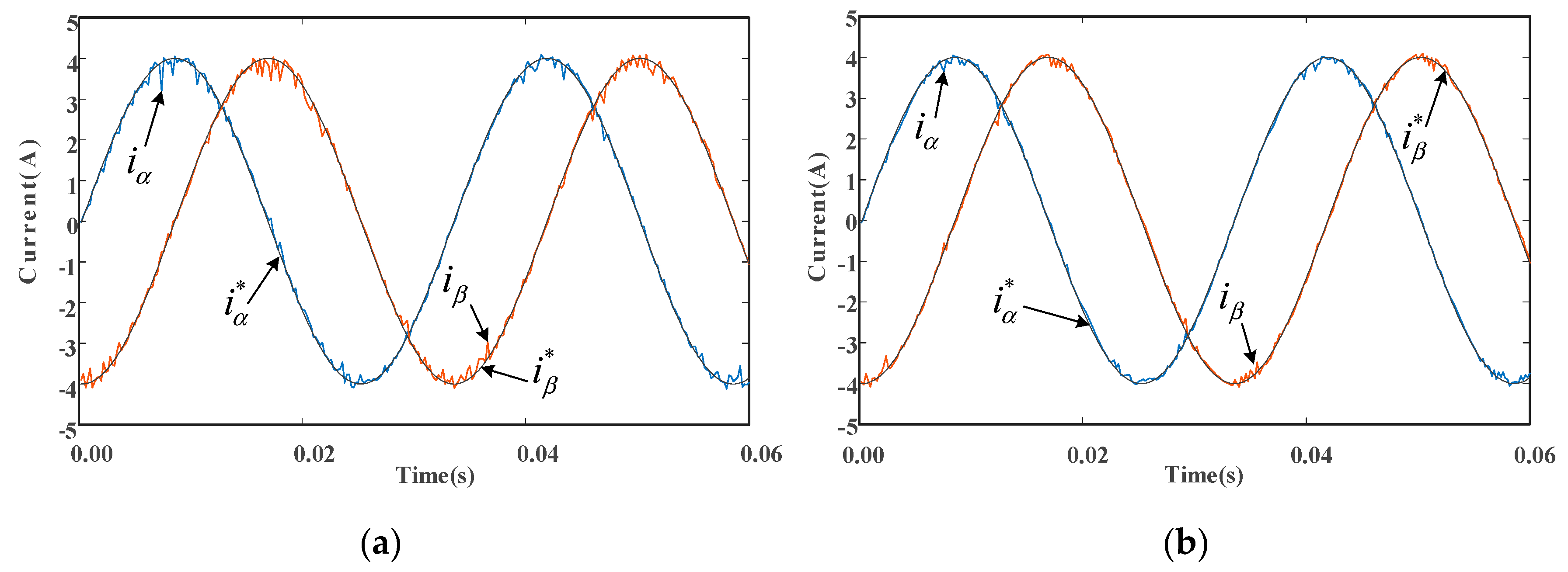
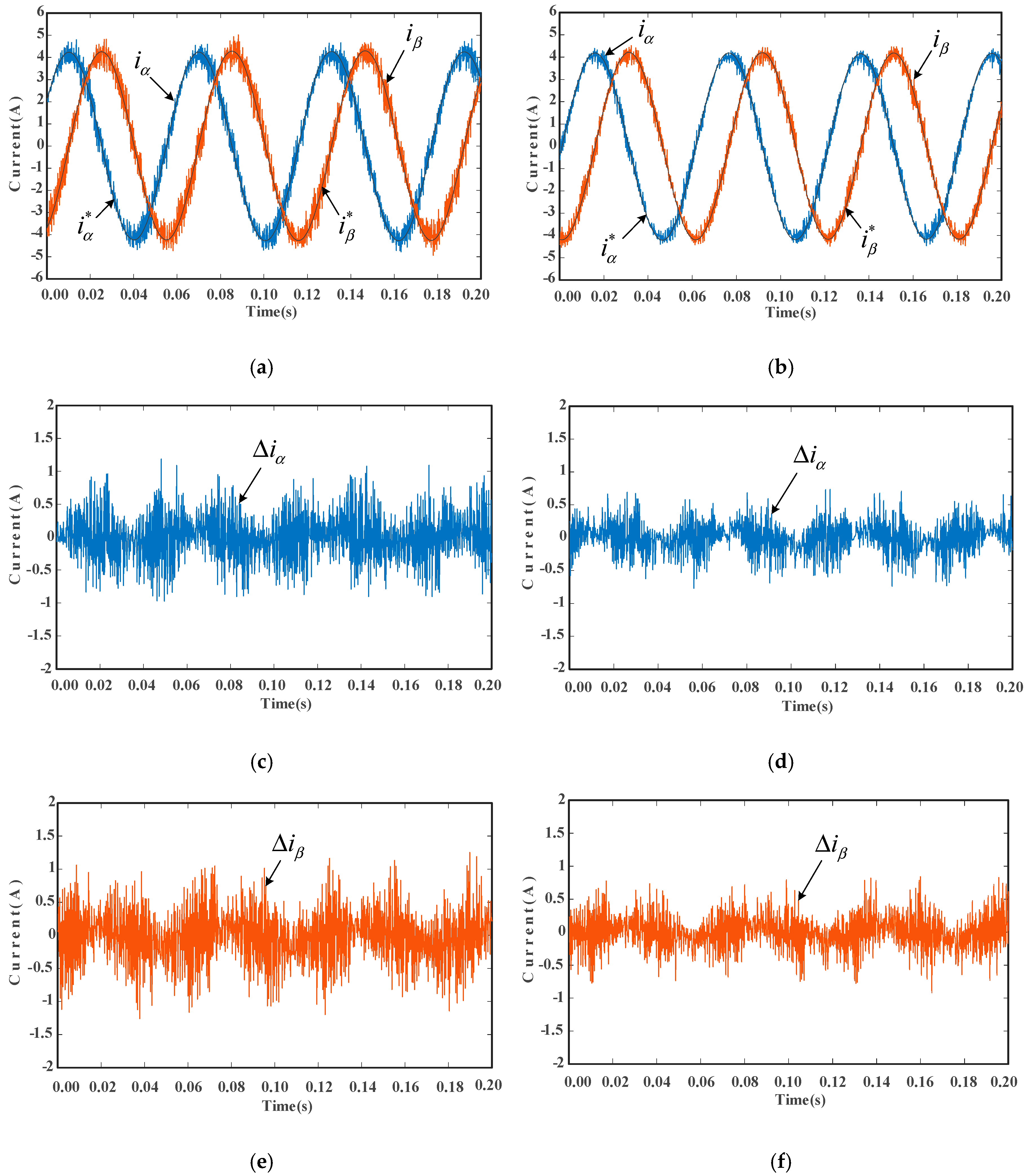
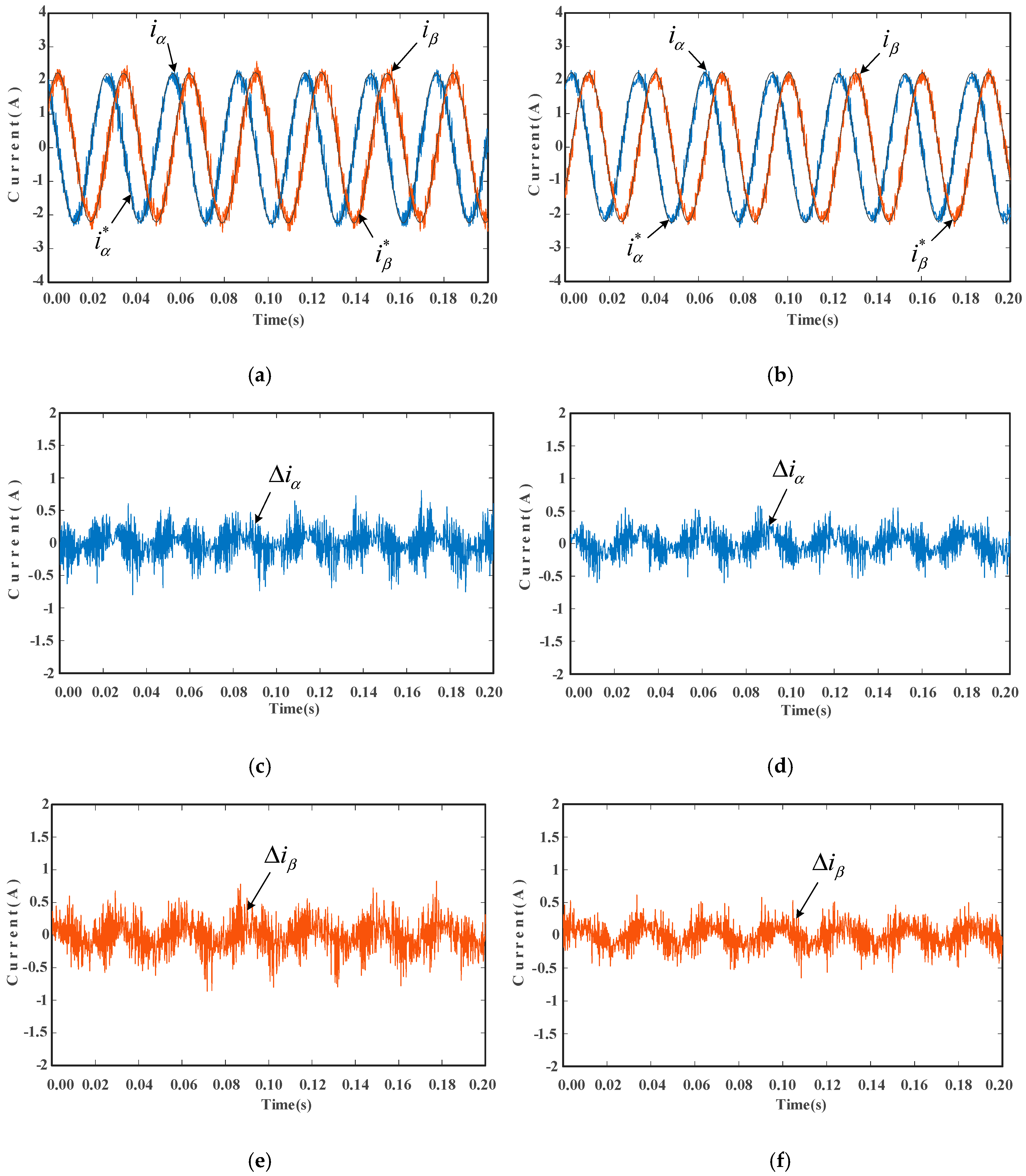
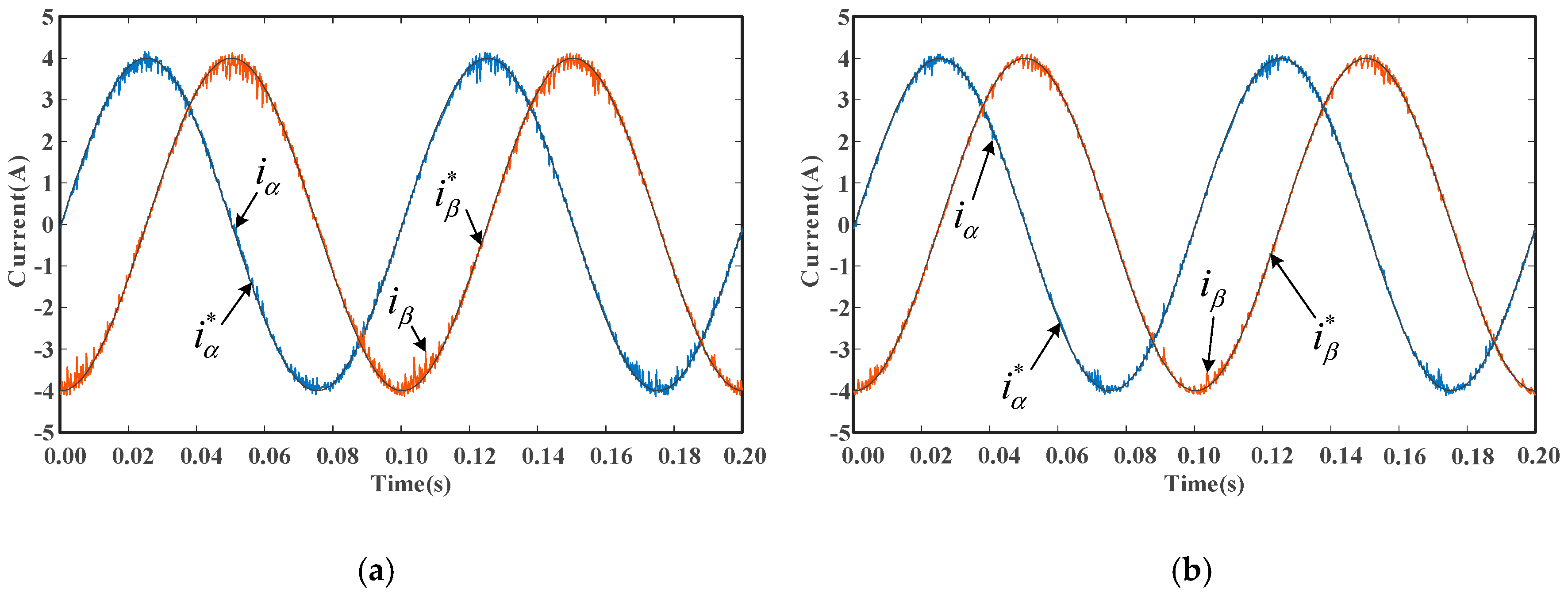
4.1. Steady-State Response

To illustrate the response of the proposed method, steady-state performance was evaluated in the α–β reference frame with stator current commands running at different frequencies. Figure 8 shows the α–β current waveforms operating at an amplitude of 4 A and frequency of 30 Hz. As can be seen from Figure 8a, significant ripples exist at current peaks. Specifically, the current ripple is 0.1077 A, and the THD is 0.0812%. Figure 8b shows that the α-axis and β-axis currents of the proposed MMPCC follow the current commands very well, with current ripple being equal to 0.0705 A, and the THD being equal to 0.0812%. In terms of the improvement made to the MPCC, the proposed MMPCC reduces the current ripple by 34.54% and decreases the THD by 41.89%, according to Figure 8.

The next experiment is for performance evaluation at a low operating frequency. The experimental results of tracking the α–β current commands with amplitude of 4 A and frequency of 10 Hz are shown in Figure 9. As can be observed, Figure 9a exhibits more pronounced current ripples at peaks compared to Figure 9b. Particularly, the current ripple and THD produced by the MMPCC are reduced by 32.92% and 11.54% in terms of the improvement made to the MPCC. These results clearly demonstrate that the proposed MMPCC has better tracking performance under steady-state operations.

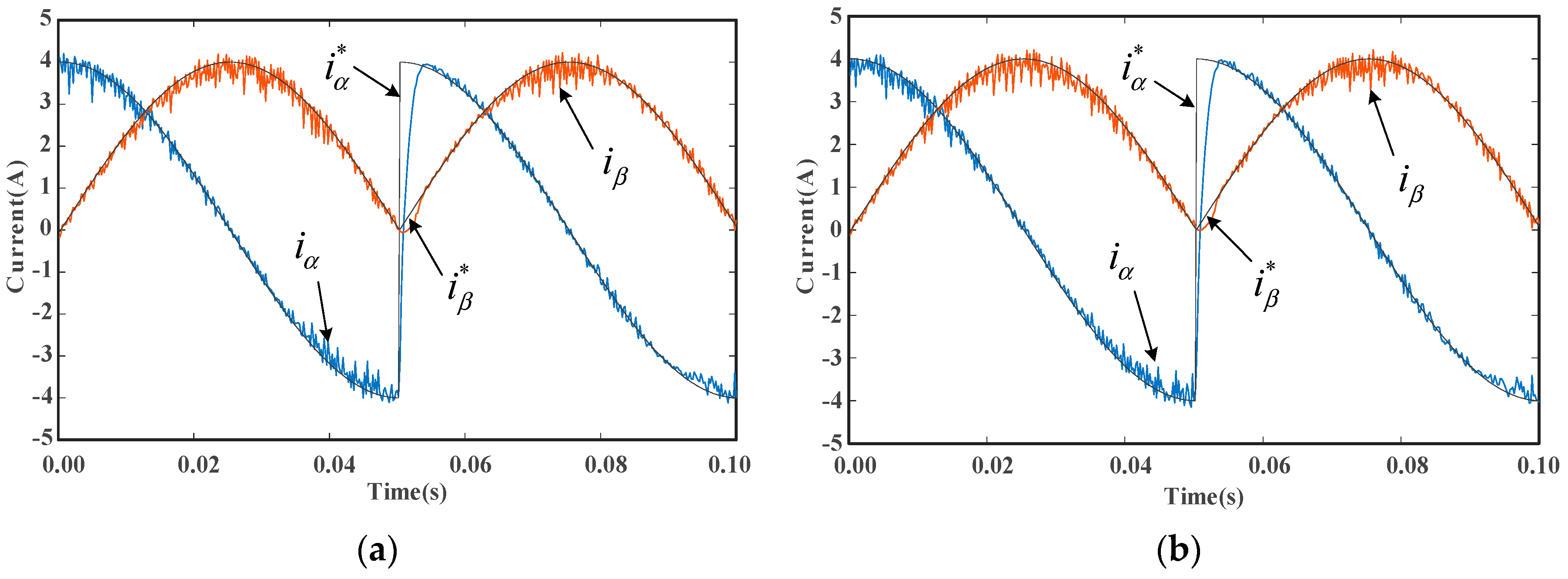
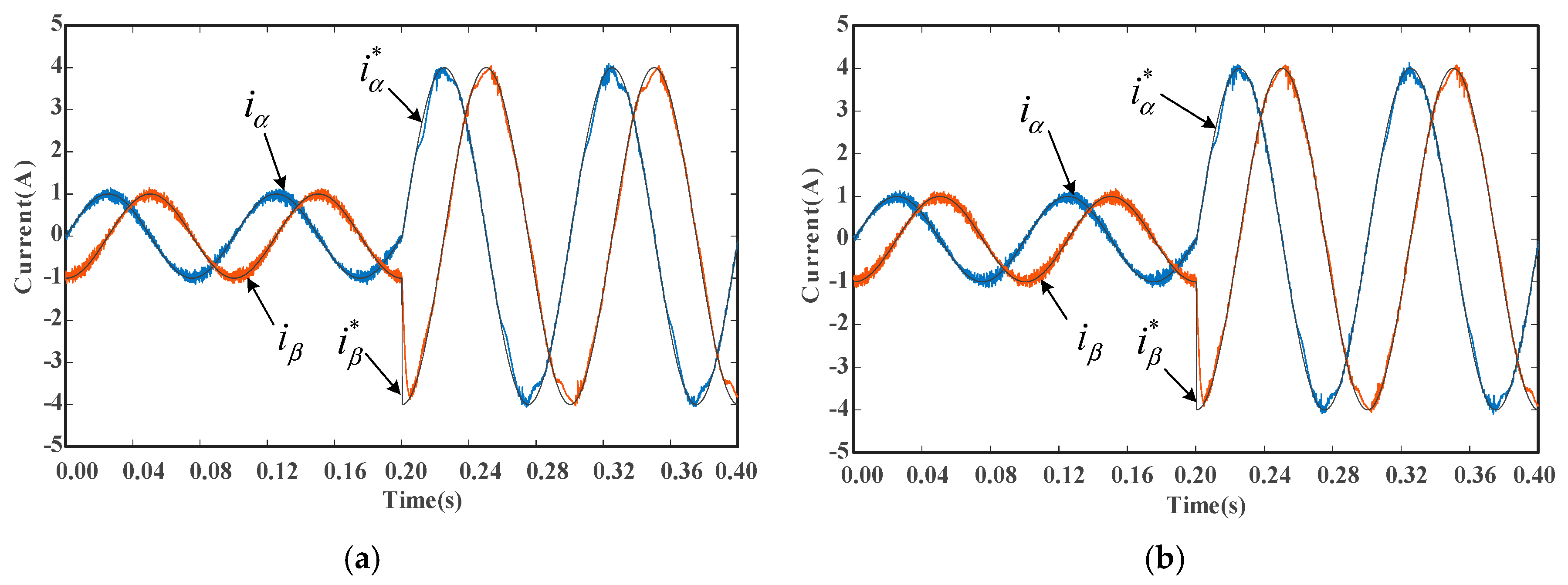
4.2. Transient Response

Among the many factors that need to be considered in terms of the operations of converters and electrical drives, two crucial ones stand out: fast response, and rejection of ambient electromagnetic disturbances. However, here, the focus is only placed on the former, as the latter is beyond the scope of this study. The transient response of the motor driver’s output current is highly dependent on the current controller. To demonstrate the performance in this regard, a simple test is conducted containing an abrupt change in the current command during operations. Figure 10 shows the instantaneous behaviors where the α-axis current command undergoes a sudden jump from −4 A to 4 A at 0.05 s. As can be seen from Figure 10, both methods exhibit good transient responses. In this test, MMPCC performed slightly better than did the MPCC without modulation. Specifically, compared with the latter, the former reduced current ripple and THD by only 1.76% and 0.15%, respectively. A possible explanation for this is that the duration of comparison was too short, at only 0.1s. Additionally, the transient current error due to the sudden change in current command is much larger than the current ripple of interest. Figure 11, on the other hand, illustrates the transient performance of α–β current command jumping from 1 A to 4 A at 0.2 s. Similar to the previous transient test, it is clearly visible that better current tracking performance is achieved by the proposed MMPCC. Current ripple is impressively reduced by 8.98%, while THD is slightly decreased by 0.68%.

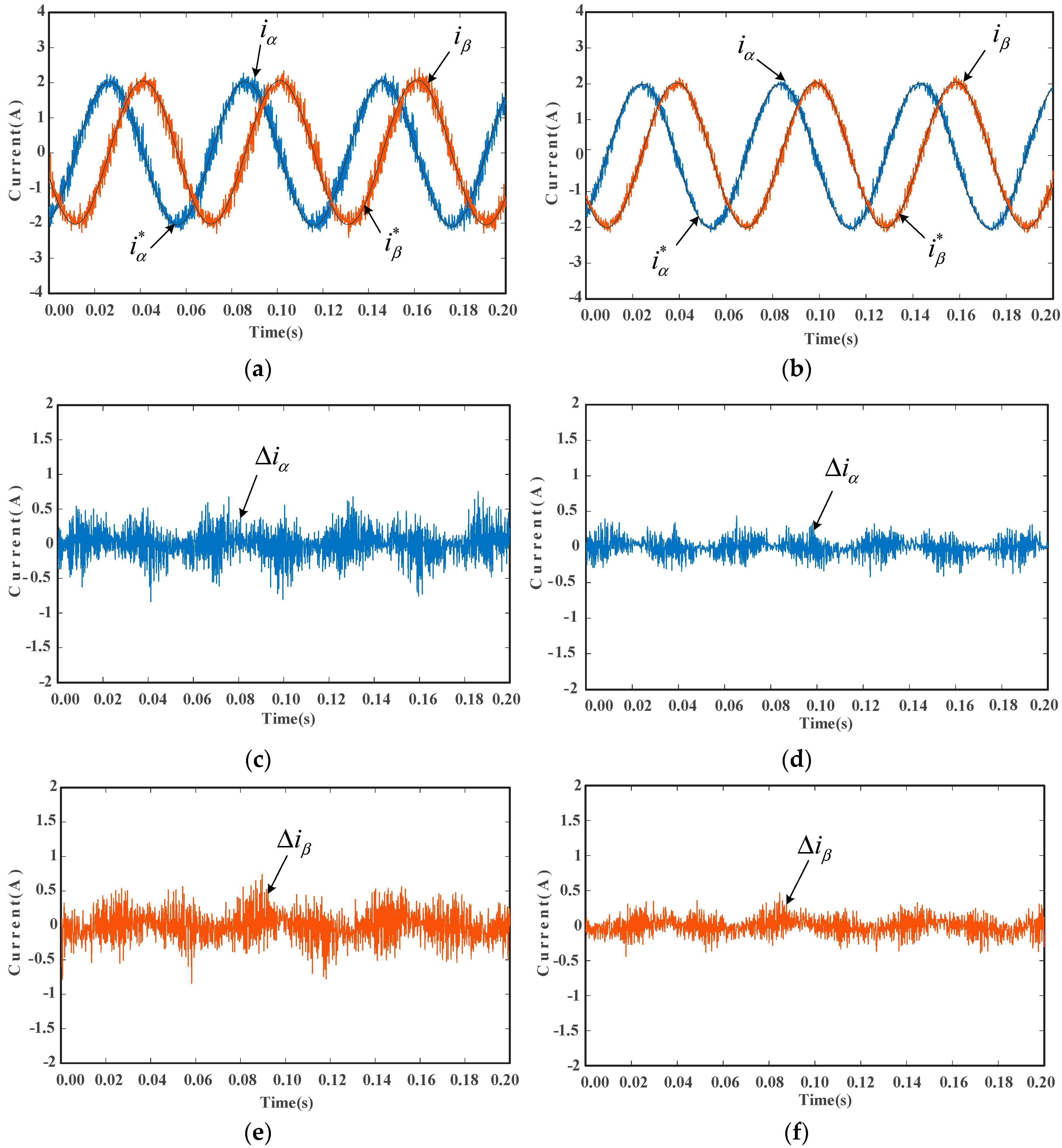
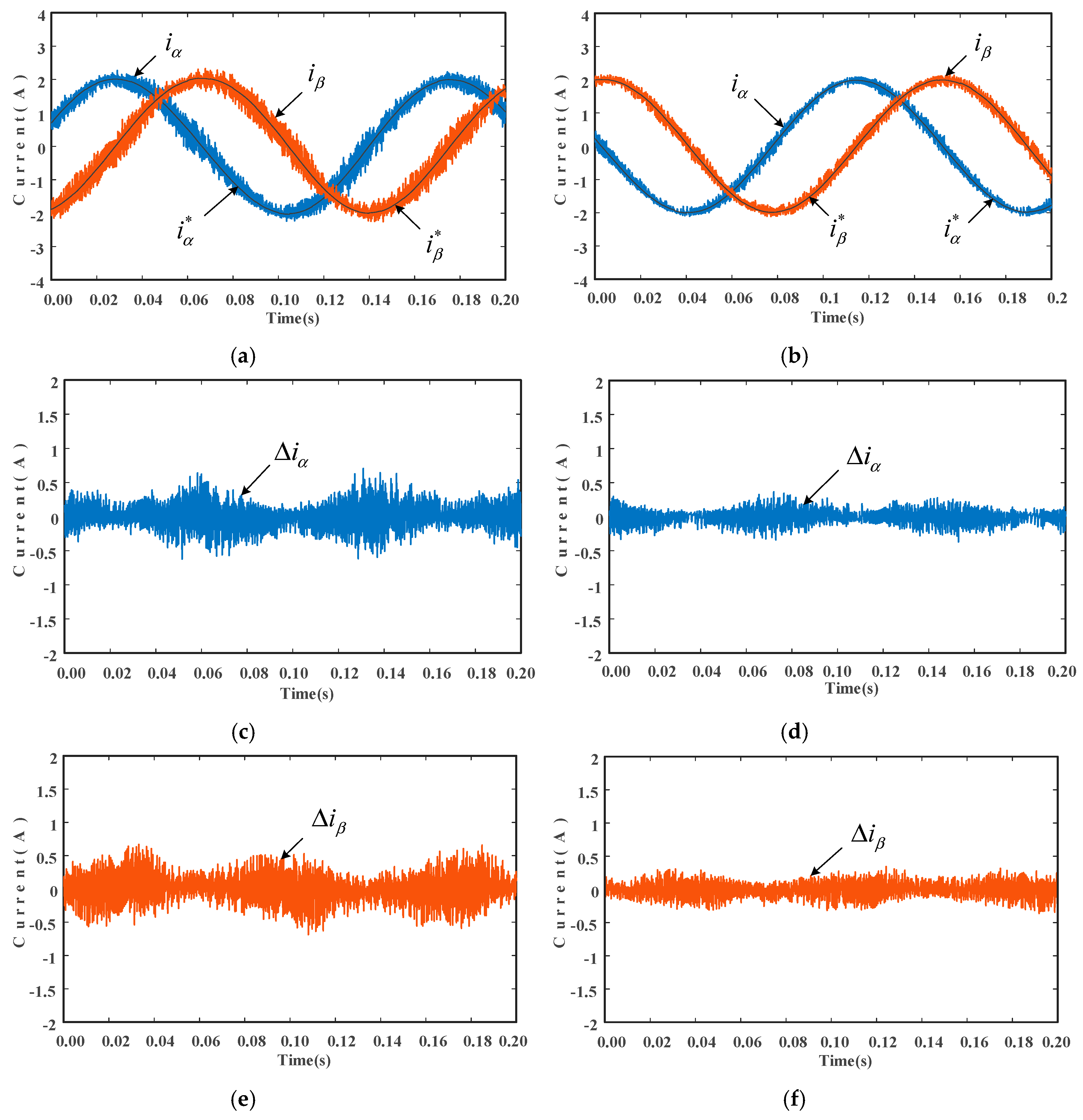
4.3. Load-Torque and Speed Varying Condition

Further evaluation is conducted at various load-torque and speed conditions. To better illustrate the difference between the two current controllers in terms of their performances under steady-state current tracking, the waveforms of α–β current errors are provided.

Given in Figure 12 and Figure 13 are the results of IPMSM running at a constant speed of 500 rpm under different load-torques of 1 N-m and 2 N-m, respectively. Figure 12a shows the corresponding current waveforms in which the MPCC generates 0.2463 A of current ripples and 5.8826% of THD. In that regard, the proposed MMPCC in yields smaller ripples and THD with high percentage performance improvements up to 44.05% and 62.29%, respectively, as depicted in Figure 12b. In addition, the current errors as shown in Figure 12d,f are significantly smaller than those in Figure 12c,e, respectively. Figure 13 illustrates the current responses of the two control schemes with the IPMSM running at 500 rpm with a load-torque of 2 N-m. The current ripple and THD of the MPCC are reduced by 34.84% and 3.24%, respectively, by the proposed MMPCC, according to the data. Figure 14 shows the results under a constant speed of 1000 rpm and 1 N-m of load-torque. As can be seen, the THD index of the proposed MMPCC is much more satisfactory. It is found that the current ripple and THD using the proposed controller are reduced by 21.49% and 1.97%, respectively, compared to the MPCC. Similar results can also be observed in Figure 15. Based on Figure 12, Figure 13, Figure 14 and Figure 15, both current controllers can perform the current tracking tasks for the IPMSM operating at 200, 500, and 1000 rpm successfully. However, the proposed MMPCC has much better current-tracking performance in significantly reducing the current errors.

4.4. Anaylsis

The experimental results are summarized in

Table 5. Quantitative summary of experimental results.

Figure	MPCC Without Modulation		MMPCC		Improvements to MPCC
	Current Ripple (A)	THD (%)	Current Ripple (A)	THD (%)	Current Ripple Reduction (%)	THD Reduction (%)
Figure 8	0.1077	0.8182	0.0705	0.4755	34.54	41.89
Figure 9	0.1136	0.7008	0.0762	0.6199	32.92	11.54
Figure 10	0.3133	17.3591	0.3078	17.3339	1.76	0.15
Figure 11	0.1447	8.6492	0.1317	8.5906	8.98	0.68
Figure 12	0.2463	5.8826	0.1378	2.2183	44.05	62.29
Figure 13	0.4260	3.6802	0.2776	3.5609	34.84	3.24
Figure 14	0.2555	7.5919	0.2006	7.4425	21.49	1.97
Figure 15	0.2166	6.7520	0.1326	3.1791	38.78	52.92

. For the steady-state tests, Figure 8 and Figure 9 depict that the current ripples are reduced by approximately 34.54% and 32.92%, respectively. On the other hand, both the MMPCC and the MPCC have good transient responses, as revealed by Figure 10 and Figure 11. Figure 12 and Table 5 show an interesting finding that the current ripple and THD using the MMPCC are reduced by 44.05% and 62.29%, respectively, compared to the MPCC without modulation. In addition, in Figure 13, Figure 14 and Figure 15, one can observe that the reductions in current ripples are up to 34.84%, 21.49% and 38.78%, respectively. Based on Table 5 one may conclude that the proposed MMPCC largely enhances the current-tracking performance of the IPMSM drive system.

5. Conclusions

An MMPCC for IPMSM is proposed and successfully implemented in this work. The new method modulates two voltage vectors in a sampling period with adaptive application durations and achieves current predictions effectively. Compared to the conventional MPC using seven cost values, the proposed MMPCC enlarges the candidate pool by employing thirteen cost values, while retaining simplicity. Through the novel design of a cost function, an optimal switching mode is obtained whose application time is optimized and calculated online. The presented experimental results demonstrate that the proposed method has good current tracking capabilities under steady-state, transient, and various operation conditions. Quantitatively, the improvements it made to the MPCC include the current ripple reduction by 27.17% and THD reduction by 21.84%, respectively, by means of averaging all data from the eight experiments, among which the highest current ripple reduction rate achieved was up to 44.05% in the best case. Thanks to the modulation and online optimization technique, the proposed MMPCC largely contributes in the reduction of current ripples and improves current tracking errors, compared to the MPCC without modulation, hence achieving significant performance improvement.

References

1. Kim, S.I.; Kim, Y.K.; Lee, G.H.; Hong, J.P. A novel rotor configuration and experimental verification of interior PM synchronous motor for high-speed applications. IEEE Trans. Magn. 2012, 48, 843–846. [Google Scholar] [CrossRef]
2. Rovere, L.; Formentini, A.; Gaeta, A.; Zanchetta, P.; Marchesoni, M. Sensorless finite-control set model predictive control for IPMSM drives. IEEE Trans. Ind. Electron. 2016, 63, 5921–5931. [Google Scholar] [CrossRef]
3. Rodriguez, J.; Cortes, P. Predictive Control of Power Converters and Electrical Drives, 1st ed.; John Wiley & Sons Ltd. Publication: West Sussex, UK, 2012; pp. 133–143. [Google Scholar]
4. Bose, B. Energy, environment, and advances in power electronics. IEEE Trans. Power Electron. 2000, 15, 688–701. [Google Scholar] [CrossRef]
5. Rodriguez, J.; Pontt, J.; Silva, C.A.; Correa, P.; Lezana, P.; Cortes, P.; Ammann, U. Predictive current control of a voltage source inverter. IEEE Trans. Ind. Electron. 2007, 54, 495–503. [Google Scholar] [CrossRef]
6. Xia, C.; Wang, M.; Song, Z.; Liu, T. Robust model predictive current control of three-phase voltage source PWM rectifier with online disturbance observation. IEEE Trans. Ind. Inform. 2012, 8, 459–471. [Google Scholar] [CrossRef]
7. Beerten, J.; Verveckken, J.; Driesen, J. Predictive direct torque control for flux and torque ripple reduction. IEEE Trans. Ind. Electron. 2010, 57, 404–412. [Google Scholar] [CrossRef]
8. Yang, X.; Liu, G.; Li, A.; Le, V.D. A predictive power control strategy for DFIGs based on a wind energy converter system. Energies 2017, 10, 1098. [Google Scholar] [CrossRef]
9. Siami, M.; Khaburi, D.A.; Abbaszadeh, A.; Rodriguez, J. Robustness improvement of predictive current control using prediction error correction for permanent-magnet synchronous machines. IEEE Trans. Ind. Electron. 2016, 63, 3458–3466. [Google Scholar] [CrossRef]
10. Bode, G.H.; Loh, P.C.; Newman, M.J.; Holmes, D.G. An improved robust predictive current regulation algorithm. IEEE Trans. Ind. Appl. 2005, 41, 1720–1733. [Google Scholar] [CrossRef]
11. Mynar, Z.; Vesely, L.; Vaclavek, P. PMSM model predictive control with field-weakening implementation. IEEE Trans. Ind. Electron. 2016, 63, 5156–5166. [Google Scholar] [CrossRef]
12. Ngo, V.Q.B.; Nguyen, M.K.; Tran, T.T.; Lim, Y.C.; Choi, J.H. A simplified model predictive control for T-type inverter with output LC filter. Energies 2019, 12, 31. [Google Scholar] [CrossRef]
13. Zhang, Y.; Xie, W.; Li, Z.; Zhang, Y. Model predictive direct power control of a PWM rectifier with duty cycle optimization. IEEE Trans. Power Electron. 2013, 28, 5343–5351. [Google Scholar] [CrossRef]
14. Yan, L.; Dou, M.; Hua, Z.; Zhang, H.; Yang, J. Optimal duty cycle model predictive current control of high-altitude ventilator induction motor with extended minimum stator current operation. IEEE Trans. Power Electron. 2018, 33, 7240–7251. [Google Scholar] [CrossRef]
15. Zhang, Z.; Zhao, Y.; Qiao, W.; Qu, L. A space-vector-modulated sensorless direct-torque control for direct-drive PMSG wind turbines. IEEE Trans. Ind. Appl. 2014, 50, 2331–2341. [Google Scholar] [CrossRef]
16. Zhang, Z.; Wei, C.; Qiao, W.; Qu, L. Adaptive saturation controller-based direct torque control for permanent-magnet synchronous machines. IEEE Trans. Power Electron. 2016, 31, 7112–7122. [Google Scholar] [CrossRef]
17. Castelló, J.; Espí, J.M.; García-Gil, R. A new generalized robust predictive current control for grid-connected inverters compensates anti-aliasing filters delay. IEEE Trans. Ind. Electron. 2016, 63, 4485–4494. [Google Scholar] [CrossRef]
18. Su, D.; Zhang, C.; Dong, Y. Finite-state model predictive current control for surface-mounted permanent magnet synchronous motors based on current locus. IEEE Access 2017, 5, 27366–27375. [Google Scholar] [CrossRef]
19. Siami, M.; Khaburi, D.A.; Rivera, M.; Rodríguez, J. An experimental evaluation of predictive current control and predictive torque control for a PMSM fed by a matrix converter. IEEE Trans. Ind. Electron. 2017, 64, 8459–8471. [Google Scholar] [CrossRef]
20. Lin, C.K.; Liu, T.H.; Yu, J.T.; Fu, L.C.; Hsiao, C.F. Model-free predictive current control for interior permanent-magnet synchronous motor drives based on current difference detection technique. IEEE Trans. Ind. Electron. 2014, 61, 667–681. [Google Scholar] [CrossRef]
21. Lin, C.K.; Yu, J.T.; Lai, Y.S.; Yu, H.C. Improved model-free predictive current control for synchronous reluctance motor drives. IEEE Trans. Ind. Electron. 2016, 63, 3942–3953. [Google Scholar] [CrossRef]
22. Lin, C.K.; Yu, J.T.; Huang, H.Q.; Wang, J.T.; Yu, H.C.; Lai, Y.S. A dual-voltage-vector model-free predictive current controller for synchronous reluctance motor drive systems. Energies 2018, 11, 1743. [Google Scholar] [CrossRef]
23. Majmunović, B.; Dragičević, T.; Blaabjerg, F. Multi objective modulated model predictive control of stand-alone voltage source converters. IEEE J. Emerg. Sel. Top. Power Electron. 2019. [Google Scholar] [CrossRef]
24. Wu, Z.; Chu, J.; Gu, W.; Huang, Q.; Chen, L.; Yuan, X. Hybrid modulated model predictive control in a modular multilevel converter for multi-terminal direct current systems. Energies 2018, 11, 1861. [Google Scholar] [CrossRef]
25. Gong, Z.; Wu, X.; Dai, P.; Zhu, R. Modulated model predictive control for MMC-based active front-end rectifiers under unbalanced grid conditions. IEEE Trans. Ind. Electron. 2019, 66, 2398–2409. [Google Scholar] [CrossRef]
26. Garcia, C.F.; Silva, C.A.; Rodriguez, J.R.; Zanchetta, P.; Odhano, S.A. Modulated model-predictive control with optimized overmodulation. IEEE J. Emerg. Sel. Top. Power Electron. 2019, 7, 404–413. [Google Scholar] [CrossRef]
27. He, Z.; Guo, P.; Shuai, Z.; Xu, Q.; Luo, A.; Guerrero, J.M. Modulated model predictive control for modular multilevel AC/AC converter. IEEE Trans. Power Electron. 2019, 34, 10359–10372. [Google Scholar] [CrossRef]
28. Lin, C.K.; Liu, T.H.; Lo, C.H. Sensorless interior permanent magnet synchronous motor drive system with a wide adjustable speed range. IET Electr. Power Appl. 2009, 3, 133–146. [Google Scholar] [CrossRef]
29. Cortes, P.; Rodriguez, J.; Silva, C.; Flores, A. Delay compensation in model predictive current control of a three-phase inverter. IEEE Trans. Ind. Electron. 2012, 59, 1323–1325. [Google Scholar] [CrossRef]
Figure 1. Diagram of three-phase six-switch voltage source inverter-fed IPMSM.
Energies 12 02885 g001
Figure 2. A diagram of voltage vectors.
Energies 12 02885 g002
Figure 3. Current prediction control of conventional MPC.
Energies 12 02885 g003
Figure 4. Applied voltage vectors in a typical sampling period: (a) conventional MPCC without modulation; (b) the proposed MMPCC.
Energies 12 02885 g004
Figure 5. Distribution of thirteen synthesized voltage vectors.
Energies 12 02885 g005
Figure 6. MMPCC schematic control diagram of stator current prediction.
Energies 12 02885 g006
Figure 7. Drive circuit of the MMPCC.
Energies 12 02885 g007
Figure 8. Trajectories of steady-state current under command 4 A at 30 Hz: (a) MPCC without modulation; (b) the proposed MMPCC.
Energies 12 02885 g008
Figure 9. Trajectories of steady-state current under command 4 A at 10 Hz: (a) MPCC without modulation; (b) the proposed MMPCC.
Energies 12 02885 g009
Figure 10. Transient response with abrupt current step from −4 A to 4 A at 0.05 s in the α -axis: (a) MPCC without modulation; (b) the proposed MMPCC.
Energies 12 02885 g010
Figure 11. Transient response with current magnitude jumping from 1 A to 4 A at 0.2 s: (a) MPCC without modulation; (b) the proposed MMPCC.
Energies 12 02885 g011
Figure 12. Currents and current errors under constant motor speed of 500 rpm and load-torque 1 N-m: (a) current responses of the MPCC without modulation, (b) current responses of the proposed MMPCC, (c) the α-axis current error of Figure 12a, (d) the α-axis current error of Figure 12b, (e) the β -axis current error of Figure 12a, and (f) the β -axis current error of Figure 12b.
Energies 12 02885 g012
Figure 13. Currents and current errors under constant speed of 500 rpm and load-torque of 2 N-m: (a) current responses of the MPCC without modulation, (b) current responses of the proposed MPCC, (c) the α-axis current error of Figure 13a, (d) the α-axis current error of Figure 13b, (e) the β -axis current error of Figure 13a, and (f) the β -axis current error of Figure 13b.
Energies 12 02885 g013
Figure 14. Currents and current errors under constant speed 1000 rpm and load-torque 1 N-m: (a) current responses of the MPCC without modulation, (b) current responses of the proposed MMPCC, (c) the α-axis current error of Figure 14a, (d) the α-axis current error of Figure 14b, (e) the β -axis current error of Figure 14a, and (f) the β -axis current error of Figure 14b.
Energies 12 02885 g014
Figure 15. Currents and current errors under constant speed of 200 rpm and load-torque 1 N-m: (a) current responses of the MPCC without modulation, (b) current responses of the proposed MMPCC, (c) the α-axis current error of Figure 15a, (d) the α-axis current error of Figure 15b, (e) the β -axis current error of Figure 15a, and (f) the β -axis current error of Figure 15b.
Energies 12 02885 g015