Assessment of Renewable Energy Deployment Roadmaps

Abstract

This research implements a methodology to the joint assessment of the photovoltaic and onshore wind investment roadmaps put forward by the main institutions in the field, International Renewable Energy Association (Irena) and the International Energy Agency, to achieve a low carbon emissions economy with near zero net greenhouse gases emissions. The two energies taken together account for over 80% of the renewable energy deployments envisaged by both roadmaps. The assessment is conducted according to economic criteria (the levelized cost of energy, capital requirements and financial risks), and environmental (carbon avoided, its value, and its cost). Given the recent Intergovernmental Panel on Climate Change (IPCC) report on the urgency to tackle climate change, accelerated deployments of the roadmaps are assessed as well. Overall, it is found that the roadmaps are financially sound, even under an accelerated scenario. Possible limits to the deployment of renewable energies roadmaps derived from the availability of raw materials and other constraints are also discussed, showing likely constraints for lithium batteries but not for photovoltaic and wind energies.

1. Introduction

This research reports the results of implementing the methodology presented in [1] to the assessment of the joint roadmaps (RM) put forward by the International Energy Agency (IEA) [2], and the International Renewable Energy Association (Irena) [3] to decarbonize the world economy by 2050. The joint report by both organizations was produced at the request of the German government for its G20 presidency in 2017 and tried to answer the specific question of designing an energy transition path that would limit the rise in global temperature well below two degrees Celsius (2 °C), as agreed in the Paris Agreement. Both institutions therefore address the same question although with different methodologies, notably the IEA includes all low carbon technologies while Irena stresses the potential of renewable energies (RE). The resulting RMs show some similarities, although significant differences due to the use of different models and tools as well. There are other published RMs tackling a similar problem although less complete: e.g., (1) Ref. [4] considers the main 138 countries accounting for most of the world energy demand, so coverage is not complete; (2) Ref. [5] is already some years old, (3) Ref. [6] only consider the power sector omitting transportation, and, (4) Ref. [7] is very similar to [5]. Many other RMs consider only specific sectors of the economy or else a limited geographical area.

In both the IEA and Irena’s RMs, photovoltaic (PV) and on-shore wind energies cover up to 80% of the renewable energy sources (RES) considered, and therefore are the main concern of the present approach. The methodology focuses on three type of questions: (1) economic and financial assessment criteria; instead of the usual net present discounted cost of the investment RM, an alternative measure called the levelized cost of energy (LCOE) is put forward as the main yardstick; total capital requirements are evaluated as well. (2) Externalities: (a) technology learning rates (LR) and the ensuing capital price decreases, (b) estimation of the CO₂ and other greenhouse gases (GHG) avoided under several assumptions relating to fossil fuels replacement; (c) the social discount rate (SDR) as a more appropriate discount rate from a global rather than a market point of view, and, (d) storage requirements and their costs implied by the inherent intermittency of RES. (3) Financial risks, mainly derived by the uncertainty in the LR equations driving capital costs as a result of increased installed capacity. The latest Intergovernmental Panel on Climate Change (IPCC) [8] report regarding the shrinking time window left to counter climate change is also reckoned: RMs with the same final targets as those set up by Irena and the IEA, but being achieved far more quickly are analyzed in detail.

The paper is organized as follows: Section 2.1 reviews the main aspects of the methodology implemented. Section 2.2, Section 2.3 and Section 2.4 discuss further the most relevant aspects of the methodology, and Section 2.5 presents and discusses with some detail both RMs analyzed. Section 3 is devoted to reporting and discussing the main empirical results: Section 3.1, LCOE and implied risks; Section 3.2, avoided carbon and its value; Section 3.3, capital prices and other costs; Section 3.4, possible constraints to the deployment and energy generated by RES. Section 4 gathers and discusses the main conclusions and points to further research.

2. Materials and Methods

2.1. The Methodology

The specification and measures implemented to assess the energy investment RMs, involving PV and wind energy are briefly commented next (a full account of the methodology is presented in [1]). The conventional economic criterion to assess RMs is their implied total net cost discounted to the present. As a complementary measure, the total amount of CO₂ avoided, and possibly other GHG are customarily given as well. A more encompassing economic measure, broadly defined as the unitary break-even price of a given energy source is the LCOE. It is conventionally implemented for the evaluation of individual energies, and it can offer a more complete perspective on the economics of a complete RM of investments as well. This is because minimizing the LCOE, i.e., the unitary break-even cost of energy, is akin to profit maximization, which is the principle under which competitive markets are supposed to work efficiently; see [9]. Even when just one single energy source is involved this implementation implies less obvious choices, the main reason being that then a social or global point of view has to be considered, which implies accounting for all possible kinds of externalities as well as the LR effect of capacity on prices. Questions derived from this global point of view, and other more economic aspects which arise from the whole series of annual investments involved are tackled in the empirical assessment reported.

Three types of related criteria are considered: (a) the unitary cost of energy as given by the LCOE and total capital expenditures; (b) avoided carbon (AC) emissions and their valuation; and, (c) risk measures. The calculation of the LCOE requires, as a first step, the specification of the LR effect on prices derived from expanding installed capacities; see [10] for PV estimates, and [11] for onshore wind estimates. Capital and remaining balance of system costs (BoS) can be derived from there with additional specifications. Energy generated is calculated accounting for the depreciation rate and lifetime of physical capital and its capacity factor. The RM assessment accounts for three main externalities: First, as an appropriate measure of discount rate, a social discount rate is implemented according to the discussion in the relevant literature—see e.g., [12]; second, storage needs implied by intermittent renewable energies and their cost are also accounted for; and finally third, energy generated by a renewable rather than by a fossil source, allows the estimation of the amount of carbon emissions avoided by that investment and their valuation according to several possible criteria.

2.2. Effective Capital Stock

Central to all calculations is the correct estimation of the effective capital stock after accounting for wearing out as discussed next. Gross investment at time t, $\Delta C_t$, given a finite maturity or lifespan of the investment, ls, will have to recover the already obsolete investment made ls periods before, i.e.,

$$\Delta C_t=\Delta R{M}_t+\Delta C_{t-ls}$$

(1)

where $\Delta R{M}_t$ is the capacity increase foreseen in the roadmap at time t, i.e., nominal investment. $C_t$ is therefore gross capital stock at time t, and denoting the rate of capital depreciation by δ, effective or net capital stock, $C{e}_t$, at t, will be given by the sum of all previous investments before the maturity date, and appropriately discounted for depreciation, i.e.,

$$C{e}_t={{\displaystyle \sum }}_{s=0}^{ls-1}\left[\Delta C_t\times {\left(1-\delta \right)}^s\right].$$

(2)

For the values $ls=30, \delta =1\%$, and a realistic capital growth rate of $g_C=15$, straightforward algebra shows that this yields a value of 92.7%, i.e., a 7.3% reduction in the value of nominal installed capacity, $C_t$. These are realistic values for PV energy: [13,14] give ls = 30, [15] ls = 25 and [16] an even lower 0.5% depreciation rate. For the IEA values $ls=25, \delta =0.5\%$, the ratio yields a slightly lower value, 90%, attesting that the correction is significant. For wind energy a study considering individual site conditions and different turbine vintages found that load factors lost 1.6 ± 0.2% of their output each year [17]. According to [17] this decay rate is similar to that of other rotating machinery and was obtained under a variety of estimation methods, all yielding very close results. Regarding the lifetime of wind investments a common accepted value in the literature is 25 years [18,19], and according to the expert survey in [20,21], it is expected to increase 20% by 2030.

The next and immediate question to be considered is the energy generated by this effective capacity at a future date in the RM proposed given by,

$$E_t=C{e}_t\times Cf\times hy$$

(3)

where, E_t is energy generated in period t, Ce_t effective capacity given in (2), Cf the net capacity factor, and $hy=24\times 365=8760$ h per year; note that if Ce_t is measured, say, in MW, E_t will be MWh, and similarly for other measurement units. The net capacity factor of a power plant, i.e., the ratio of its actual output over a period of time to its potential output operating at full nameplate capacity continuously over the same period, varies significantly among different locations in the world, both for PV and wind energies. Although a world average is dependent on the specific locations where the facilities are located, institutions like Irena [22] have been tracking this measure for several years and their results show that it was close to 20% in 2014 for PV and slowly increasing over time, because of sunnier locations selected for the PV facilities and other minor efficiency improvements. Irena [22] concludes that it will increase linearly to reach 25% in 2030 and will stay fixed at that value thereon. As for wind energy, Irena [18] gives a world average of 28% in 2015 for the capacity factor and the expert surveys in [20,21], suggest a 10% increase in 2030: these are the values applied in the empirical simulations reported (see Appendix A for a summary).

2.3. Avoided Carbon

The total amount of AC emissions is a relevant measure for assessing an investment RM being given as,

$$AC=k^C\times {\displaystyle \sum }_{t=1}^H{E}_t$$

(4)

where, E_t is energy generated and k^C is a measure of CO₂ avoided per unit of energy generated, e.g., kilograms of CO₂ per kWh. If E_t is measured in kWh and k^C in kilograms per kWh accordingly, then $\left(0.001\times AC\right)$ gives the total amount of avoided CO₂ tons which is a standard measurement unit. Similar values, according to different sources, for coal emissions, k^C, are reported in the literature: e.g., the IPCC gives 0.82 kgCO2eq/kWh [23], and the IEA 0.78 [24].

A related measure is the avoided carbon value (ACV) for the whole roadmap given by,

$$ACV=k^C \times {\displaystyle \sum }_{t=1}^H \left(E_t\times P_t^c\right)$$

(5)

where, $P_t^C$ is the unitary price of the chosen measure for carbon, e.g., USD per kg of CO₂, which simplifies to $ACV=\left(P^c\times AC\right)$ if $P_t^c=P^c$, i.e., is constant. A thorough and recent survey on methods for pricing carbon from the global point of view, or social cost of carbon (SCC), is reported in [25]. The extensive literature survey that they provide yields minimum values of 6.7 and 14.7 USD per tons of CO₂ for the years 2015 and 2050 respectively. Maximum values are also reported but are considerably higher than average values common in the literature so that, finally, a rather conservative choice suggests selecting the minimum values provided in the survey discussed [25]. Carbon taxes provide another complementary measure, since they are the immediate cost from the individual perspective as opposite to the global point of view of the SCC. A recent and thorough report conducted on behalf of the World Bank (WB) by Stiglitz and Stern [26] suggests the values 40 to 80 USD/tCO2eq in 2020, and 50 to 100 USD/tCO2eq beyond 2030. Both valuation methods are implemented in the empirical results.

2.4. Risk Measures

A further set of questions which derive from the uncertainty of the statistically estimated LR parameters and equations relate to risk, and specifically to financial risks. Given that the available LR parameters are estimated and therefore are random, so are all simulated future values involving them, and specifically the LCOE and capital expenditures. This uncertainty cannot be avoided although it is possible to implement measures to control it. Two basic risk control measures proposed in the literature are the value at risk (VaR) and the expected value at risk (EVaR). 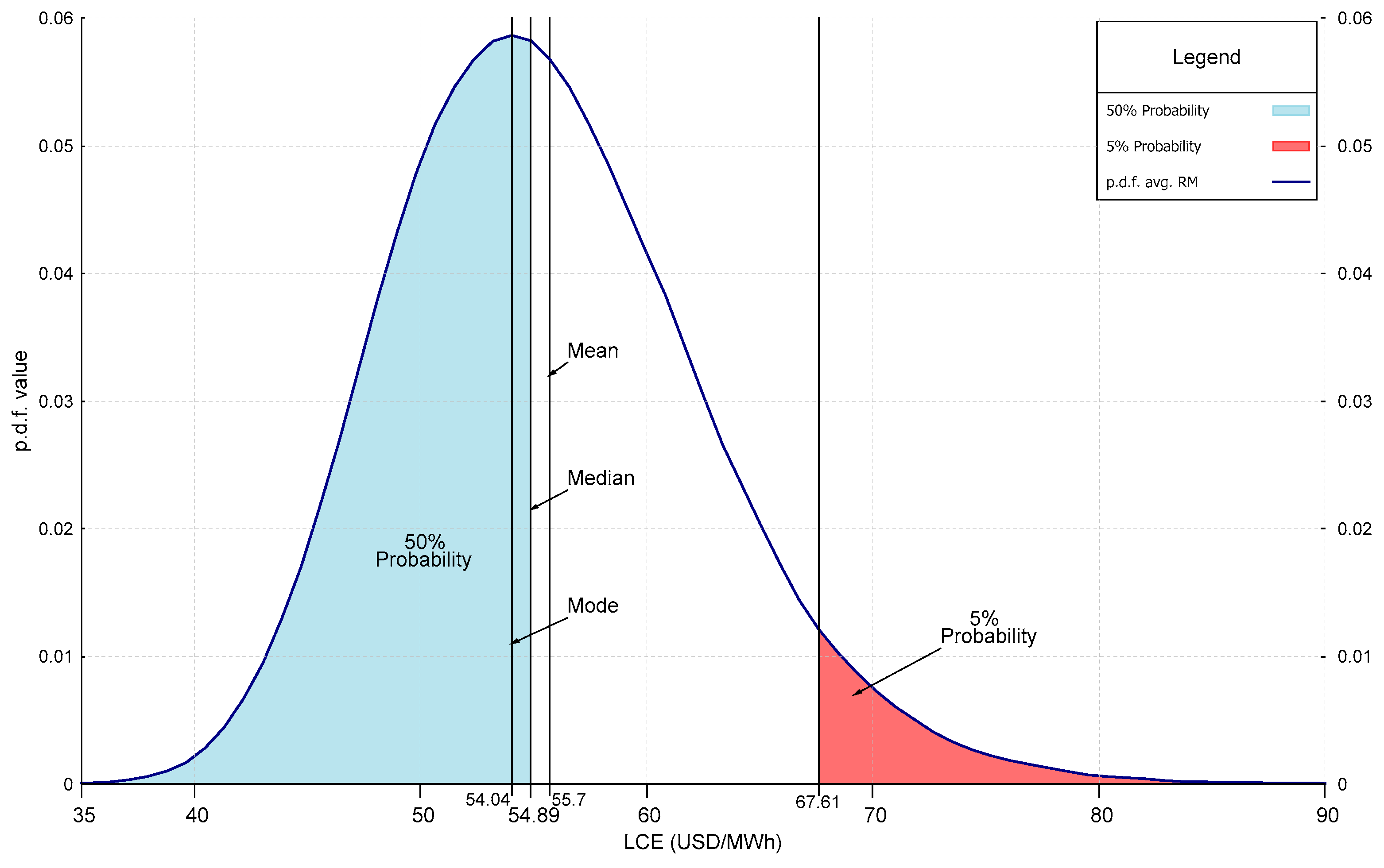The equivalent measures in this context are the LCOE or capital expenditures at risk (AR), and expected at risk (EAR); see [11,27]. Given a probability value, e.g., 95%, LCOE AR, ($\overline{LCE}$), is the highest value that the LCOE can reach within that probability, i.e.,

$$Pr\left[LCE\le \overline{LCE}\right]=0.95$$

(6)

and similarly for capital expenditures. LCOE expected at risk ($LCE\left(EAR\right)$) in turn is defined by,

$$LCE\left(EAR\right)=E\left[LCE|\left(LCE\ge \overline{LCE}\right)\right]$$

(7)

and yields the expected average value of the LCOE, should the unlikely event of the LCOE rising above the 95% limit happen. As such, it is a complementary measure to the AR value. An entirely similar analysis applies to capital expenditures. A further derived risk measure is the ratio of the expected value at risk over the average value: This provides a gauge of the maximum risk as a proportion over the expected value. Both measures are applicable to the LCOE and the financial capital requirements.

2.5. The Roadmaps Analyzed

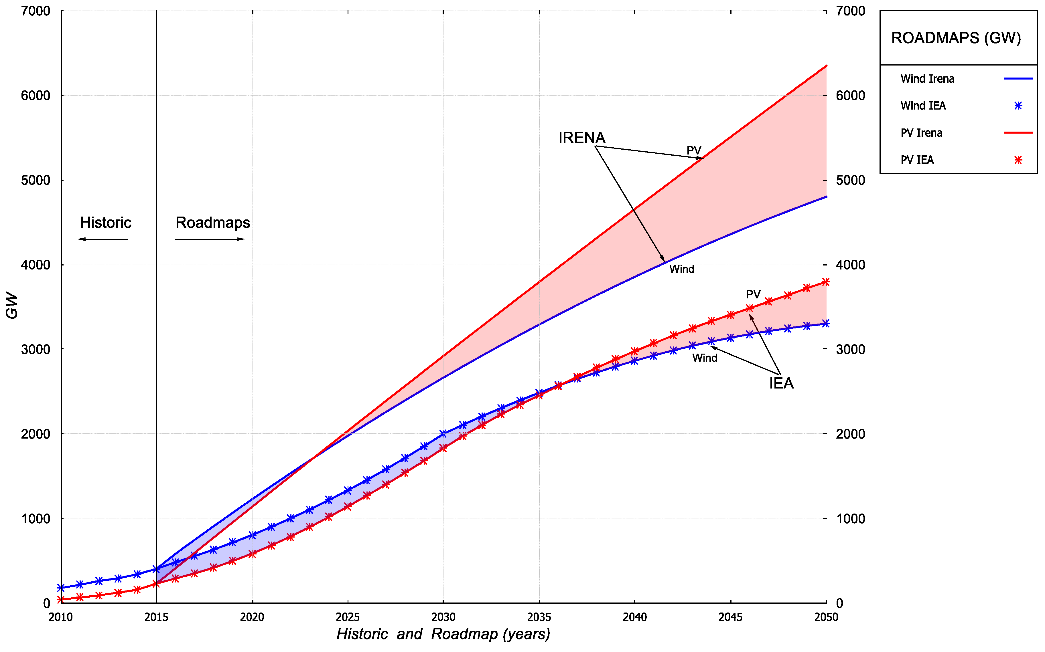
The Irena and IEA RMs for both PV and wind energies are presented in Figure 1. Both assume a departure from historic values with increased growth rates, almost linear in Irena’s case; both also assume higher rates and end values for PV than for wind, more so towards the end of the period considered. Finally, Irena’s RM is more ambitious, since it does not rely on nuclear energy and only marginally on carbon capture and storage technologies (CCS), whereas the IEA does (see Appendix A for a summary).

Accelerated RMs are considered, taking as given the end 2050 capital deployment values, ${\overline{C}}_{2050}$, and imposing a constant linear investment, so that the end targets are achieved in 2030. Several accelerated RM profiles are discussed in [9], the main conclusion being that the end RM date is far more relevant to the criteria discussed than the specific profile, and therefore a linear investment profile is not a significant restriction on the results. This accelerated deployment would match the IPCC warning concerning the just 12 years remaining to decarbonize the economy [8]. For comparison purposes delayed RMs are considered as well, assuming that no investment is conducted till 2030, being constant from then on to achieve the specified RM end values in 2050. It should be remarked that most published RMs forecast approximate constant linear investments with the exception of [4] which assumes an 80% deployment of its final targets for 2030. More specifically, the RMs can be completely specified by the following set of equations:

$$accelerated: \Delta C_t=\{\begin{array}{l}\left({\overline{C}}_{2050}-C_{2015}\right)/15, t=\left(2016,\dots ,2030\right)\\ 0, t=\left(2031,\dots ,2050\right) \end{array}$$

(8)

$$delayed: \Delta C_t=\{\begin{array}{l}0, t=\left(2016,\dots ,2030\right) \\ \left({\overline{C}}_{2050}-C_{2015}\right)/20, t=\left(2031,\dots ,2050\right)\end{array}$$

(9)

3. Results

3.1. LCOE

Table 1. Levelized cost of energy (LCOE) [USD/MWh]: Values and risk analysis. Value at risk (VaR) and expected value at risk (EVaR).

Yardsticks	IRENA			IEA
	I	II	III	I	II	III
(a)	Averages for the Roadmap
Average	52.1	53.2	48.4	55.7	56.6	52.4
VaR	63.4	64.3	59.6	67.6	68.6	64.5
EVaR	66.5	67.9	63.0	72.2	72.9	68.6
(b)	Year 2050
LCOE	38.6	38.9	39.0	43.3	42.5	42.6
VaR	49.6	50.0	50.2	55.5	54.7	54.9

Notes: (1) I, standard; II, accelerated deployment; III, delayed deployment. (See Equations (8) and (9), and Section 2.5); (2) VaR, EVaR at 95% probability interval. (See Equations (6) and (7), and Section 2.4). Meaning of colors: blue, favorable outcome; orange, acceptable value; red, risk warning; green, best outcome under specific assumptions.

reports the main results of the analysis, both for specific LCOE values and their implied risks. It is to be noted first, that the average LCOE value for the overall RM is substantially below the starting value in 2016 (82 USD/MWh), and that the final value in 2050 is even lower; both values are given in Table 1 column I, and are highlighted in blue. These results hold overall for both RMs, being more pronounced for the Irena case: Since the Irena RM assumes larger deployment values for both energies, the immediate implication is that increased RE targets do not necessarily yield increased costs. A second result can be drawn from the comparison to current electricity prices: In Europe, e.g., for 2016 Eurostat [28] gives the average values 81 EUR MWh for industries and 205 EUR for households (97, 246, USD with a 1.2 USD per EUR rate, respectively). These values are higher for industries and far higher for households, even under the worst-case scenario as reported in the last row of Table 1, for all cases and both RMs.

Considering next, a straightforward accelerated path, perhaps the most strikingly noticeable result is that the overall LCOE values only increase slightly: Table 1 column II, highlighted in orange; this has to be weighed nevertheless, against the results for delayed deployments which yield somewhat lower average cost values: Table 1 column III, highlighted in green. The overall conclusion may be that strongly accelerating the RE deployments increases costs slightly, whereas strong delays do not yield significant cost advantages. As for risks, the VaR and EVaR values in all cases lie in the range 20–30% higher than their corresponding averages, and although significant they are not large enough to jeopardize the investment plans - highlighted in red in Table 1 column I.

Figure 2 depicts the probability density function (p.d.f.) for the average LCOE of the IEA RM: the VaR is given by the right-hand side 5% probability, highlighted in light red, yielding 67.6 USD/MWh as reported in Table 1 column I. It is worth noticing as well that the median value, 54.9 USD/MWh, lies below the average (55.7 USD/MWh): This is a result of the right skewness of the p.d.f. underlining that a better centrality cost estimation is somewhat lower.

Next, Figure 3 portrays the timeline of the LCOE p.d.f. for the IEA RM. The mode of the p.d.f., i.e., its highest value, as a centrality measure of the LCOE decreases along time: This is a result of the increased capital deployed, and the implied lower capital costs because of the LR effects. Figure 3 also highlights the shrinking p.d.f. along time, implying smaller derived values for both the VaR and the EVaR respectively. It is worth remarking therefore that the uncertainty of the simulations decreases for more distant periods, although further analysis shows that the ratio of interval probabilities to the average of the distribution stays approximately constant.

Finally, Figure 4 displays the relative contribution of both energies to the main economic yardsticks, i.e., average LCOE for the RM and risk values implied by the p.d.f.’s. As before, only the distribution of the IEA RM is analyzed since the Irena case is entirely similar. The upper side shows first that the average LCOE for the PV energy is significantly lower than for the wind energy; the width of the distributions is more alike nevertheless. The lower side displays the implied accumulated probabilities, showing again that the risks implied by the wind energy are higher than those of the PV energy. The overall conclusion is that wind energy increases the overall costs and risks of the RM. Although a significant result, it does not imply that wind energy should be neglected, since there are complementary issues regarding intermittency and resource availability constraints depending on the specific sites where energies are deployed.

3.2. Capital Expenditures and Avoided Carbon

Total capital expenditures for the overall RM are given in

Table 2. Energy generated and capital expenditures.

Yardsticks	IRENA			IEA
	I	II	III	I	II	III
(a)	Energy Generated [PWh]
Total	362.1	457.9	267.1	227.4	292.7	173.7
(b)	Total Expenditures [tr. USD]
Average	18.9	24.4	12.9	12.7	16.6	9.1
at Risk	23.0	29.4	15.9	15.4	20.1	11.2
Exp. at Risk	24.1	31.1	16.8	16.4	21.3	11.9

Notes: (1) I: standard; II: accelerated deployment; III: delayed deployment. (See Equations (8) and (9), and Section 2.5); (2) VaR, EVaR at 95% probability interval. (See Equations (6) and (7), and Section 2.4); (3) All discounted to present values (Energy and expenditures). (4) SCC, social cost of carbon; S.S., Stern-Stiglitz [26]. (5) PW = 10⁹ MW; 1 tr. = 1 T = 1000 G. Meaning of colors: blue, favorable outcome; orange, acceptable value; red, risk warning; green, best outcome under specific assumptions.

b column I, and although significant they are not excessive when compared to world investment figures, highlighted in blue: e.g., world GDP in 2017 was 81 tr. USD according to the World Bank, and considering the maximum value for capital expenditures given by the accelerated case for the Irena RM reported in Table 2b column II, i.e., 31.1 trillions, that implies a 1.2% GDP investment per year, to be compared with the approximate 20% GDP annual investment actually observed data. It must be noted though, that for the accelerated deployment case capital expenditures rise considerably: Table 2b column II, highlighted in orange, almost doubling the figure for the delayed case: Table 2b column III, highlighted in green. These results must be matched with the total energy generated by the RM in both cases though, reported in Table 2a: As expected, now the balance becomes the opposite, showing much higher values for the accelerated deployment. The pattern of risk values is similar to the LCOE, being in all cases in the 20–30% range above the corresponding averages.

The values reported in

Table 3. Avoided Carbon (AC) and avoided crabon value (ACV).

Yardsticks	IRENA			IEA
	I	II	III	I	II	III
(a)	Avoided Carbon [tr. tons of CO2e]
Total	0.282	0.357	0.208	0.177	0.228	0.135
(b)	Avoided carbon value [tr. USD]
SCC	3.79	4.36	3.21	2.34	2.80	2.07
S.S.	20.6	25.8	15.6	13.0	16.5	10.1
(c)	Avoided Carbon Value (S.S.)/Expenditures (avg.)
Profit ratio	1.09	1.06	1.21	1.02	0.99	1.11

Notes: (see notes to Table 2).

a,b, allow a final economic valuation of the environmental benefits of the roadmaps: valuing the carbon avoided at moderate values, as those suggested by Stern-Stiglitz [26], the value generated by one USD investment is higher than one: Table 3c, column I, highlighted in green. This underlines the pure economic profitability of the RMs from the environmental point of view, without accounting for the many other benefits of RES.

Further insights into the contribution to tackle GHG emissions can be gathered from the analysis of the years added by the RMs till the carbon budget (CB) is exhausted, assuming that emissions continue in a business as usual (BAU) fashion: [3] gives 880 Gt CO₂ for the remaining CB, which, after applying a correcting factor to account for other GHG, would lead to an estimate of 1300 Gt CO₂e—the implied correction is derived by dividing total GHG emissions in 2017 over CO₂ emissions; see e.g., [29]. A closer estimate according to the last IPCC report would be 500 Gt CO₂, equivalent to 740 Gt CO₂e.

Table 4. Avoided carbon and increased carbon budget.

Yardsticks	IRENA			IEA
	I	II	III	I	II	III
(a)	Avoided Carbon [Gt CO2e]
Roadmap	282	357	208	177	228	135
(b)	n° of Years Added to the Carbon Budget
Avg. emissions	5.3	6.7	3.9	3.3	4.3	2.5
Coal emissions	8	10	5.8	5	6.5	3.7

Notes: (1) If the CB is 1300 Gt CO₂e, then 24 years left under BAU; (2) If the CB is 740 Gt CO₂e, then 14 years left as BAU.

reports the results assuming first that REs replace an average of the current energy system, and second assuming that coal is the energy replaced. This last assumption may be justified since coal is precisely the main energy that is already being phased out in the economy. Compared to the available years implied by both CBs considered, the immediate implication is that the extra years added are enough to meet the 2050 deadline for the [3] estimate, but not for the IPCC’s CB estimate: This implies, in turn, that more expansive and accelerated deployment RMs should be considered.

3.3. Capital Costs

The cost of one W of capital according to the wind and PV RMs in both cases is reported in

Table 5. Capital prices [USD/W].

Year	IRENA	IEA
2015 (avg.)	1.30	1.30
2050 (avg.)	0.626	0.729
At risk (2050)	0.874	1.010

Notes: (1) Avg., averages; (2) at risk, 95% prob.

: In both cases the value approximately halves by 2050, and the VaR is less than 30% higher than the corresponding average. This matches a similar result obtained for the LCOE and reported in Section 3.1, concerning the approximate halving of the LCOE in 2050 compared to its 2015 value.

A visual display of the main cost components along time is depicted in Figure 5. It is worth pointing out that in spite of the significant decrease of capital costs, as highlighted in Section 3.1 and Section 3.2, the relative weight of all cost components remains unaltered to a large extent. This implies in particular, that BoS are expected to decrease along with capital costs, a result that is supported by historical observation.

It should be noted as well, that the so called ‘stranded assets’ as defined e.g., by the IEA [30], are other costs implied by the implementation of renewable energy RMs. As a matter of fact, although the deployment of carbon capture and storage (CCS) technologies provide some degree of asset protection for fossil fuelled power plants, the IEA [2] reckons a total worth of 320 billion USD worldwide up to 2050 in terms of fossil fuelled power plants that would need to be retired prior to maturity. The IEA warns also that if action were delayed to 2025, the value of stranded assets would roughly triple enhancing the urgency of early RES deployment.

3.4. Limits to Renewables Energies

As the prospects for RES deployment required to counter warming weather increase, so does the demand for required input raw materials. This might imply supply side restrictions of several kinds, and some relevant results are discussed next. First, land availability might be an issue since there are several competing uses for it. Regarding PV energy, some straightforward results show that even under unfavorable assumptions they are mild: e.g., considering 2 ha per MW PV, the land requirements in both IEA and Irena RMs are less than 4% of the available world desert land [31]. As for wind, that is not a special constraint since the area under the turbines could be used, or else turbines are frequently located in otherwise unusable land, e.g., at high altitudes.

There is not a question about the availability of sun energy to supply world energy demand (WED) many times over; this might be an issue for wind energy, though, given that the total kinetic energy in the atmosphere is upper bounded. Agreed reported values in the literature downplay this issue nevertheless: A lower range estimate gives the availability at 2.5 times the WED [32], and others even suggest a 25 times multiple [4].

Regarding the availability of critical raw materials, a recent study [33] focusing mainly on batteries and electric vehicles (EV) concludes that only cobalt may be scarce and become politically sensitive, since extraction and refining are concentrated in just two countries, Congo and China. Their study assumes that demand for EV increases massively and ends in 2025, so that there would be much uncertainty left beyond that date. Another recent and broader study [34], based on a thorough assessment of the literature concludes that estimated values for various metals and renewable technologies vary widely, and that in particular the so called rare-earths are abundant, although their extraction costs might be high. The study notes also that regarding PV and wind energies, the broad agreement in the literature does not foresee any constraint regarding the availability of the metal supply. It must be underlined finally, that the previous conclusions have been obtained assuming a zero-recycling rate, an issue that is likely to be overcome partially in the near future.

The overall conclusion is therefore, that the main supply shortages are forecast for materials required for batteries and EV, a hurdle that will require a redesign of the transportation system, although solution proposals are already available [35,36]. The eventual discovery of new substitutes, materials and technologies, should not be underestimated either.

4. Discussion

The two roadmaps analyzed to decarbonize the world economy, (1) are feasible from an economic point of view, (2) deliver energy prices lower than current values at the end roadmap dates, (3) demand a volume of financial funds and imply risks derived from several kinds of uncertainties manageable, and (4) are environmentally profitable from a pure economic standpoint. The Irena RM, being more ambitious in wind and PV capacity deployments, delivers better outcomes in terms of the lowest energy cost as measured by the LCOE, and the largest savings in avoided carbon. The downside is the higher required capital expenditures, which make the IEA RM more feasible from this point of view.

Taking into account the latest IPCC report accelerated deployments in just twelve years have also been considered—the broad result being that the levelized cost of energy only increases slightly—this underlines the conclusion that at least from an economic standpoint it is still feasible to reach ambitious carbon reduction targets. Interestingly, the analysis of slow deployments does not yield significantly lower costs, while yielding substantially diminished environmental benefits: This suggest that the economic optimization of energy system designs should focus on the final roadmap date, rather than on the specific path leading to it. Early research along these lines is already being conducted, applied to single countries [37] and to the development of general methods [38].

Supply side constraints might arise in the implementation of the roadmaps, but close scrutiny of land, energy, and raw metals availability only point to the need for a redesign of the transportation system. This is not a straightforward issue however, although solution proposals have already been made. Finally, more expansive and accelerated targets for renewable energy deployments might be needed to limit greenhouse gases emissions.

The roadmaps discussed assume substantial population and real economic increases along the whole period, relying on projected energy savings to yield final energy needs similar to current values. These savings are appreciably higher than historical trends would suggest, so that their implementation would entail significant economic changes. Coupled with recycling requirements, they will require a transition from the growth oriented linear economy, based on consumption and discarding of used equipment to one based on moderate growth focused on the service economy.

Finally, the carbon avoided only adds a few years to the constraints implied by the carbon budget, so that there is room for considering more expansive roadmaps than those envisaged up to now. In fact, and given the urgency to tackle a warming climate, roadmaps are being increasingly published and the methodology implemented here could be a useful assessment tool.

References

1. Mauleón, I. Assessing PV and wind roadmaps: Learning rates, risk, and social discounting. Renew. Sustain. Energy Rev. 2019, 100, 71–89. [Google Scholar] [CrossRef]
2. OECD/IEA. Perspectives for the energy transition-Investment needs for a low carbon system, Chp. 2. OECD/IEA and Irena. 2016. Available online: http://www.irena.org/DocumentDownloads/Publications/Perspectives_for_the_Energy_Transition_2017.pdf (accessed on 30 May 2019).
3. Irena. Perspectives for the energy transition-Investment needs for a low carbon system, Chp. 4. OECD/IEA and Irena. 2016. Available online: http://www.irena.org/DocumentDownloads /Publications/Perspectives_for_the_Energy_Transition_2017.pdf (accessed on 30 May 2019).
4. Jacobson, M.; Delucchi, M.; Bauer, Z.; Goodman, S.; Chapman, W.; Cameron, M. 100% Clean and Renewable Wind, Water, and Sunlight All-Sector Energy Roadmaps for 139 Countries of the World. Joule 2017, 1, 108–121. [Google Scholar] [CrossRef] [Green Version]
5. Teske, S. Energy Evolution: A Sustainable World; Greenpeace International: Hamburg, Germany, 2015; Available online: https://www.researchgate.net/publication/310018861_Energy_Revolution_-_A_sustainable_world_energy_outlook_2015 (accessed on 10 June 2019).
6. Breyer, C.; Bogdanov, D.; Aghahosseini, A.; Gulagi, A.; Child, M.; Oyewo, A.; Farfan, J.; Sadovskaia, K.; Vainikka, P. Solar photovoltaics demand for the global energy transition in the power sector. Prog. Photovolt. Res. Appl. 2018, 26, 1–19. [Google Scholar] [CrossRef]
7. Teske, S. Achieving the Paris Climate Agreements Goals; Springer Open: Berlin, Germany, 2017. [Google Scholar] [CrossRef]
8. IPCC. An IPCC special report on the impacts of global warming of 1.5 °C above pre-industrial levels and related global greenhouse gas emission pathways, in the context of strengthening the global response to the threat of climate change, sustainable development, and efforts to eradicate poverty. In Global Warming of 1.5 ºC; IPCC: New York, NY, USA, 2019; Available online: http://www.ipcc.ch/pdf/special-reports/sr15/sr15_spm_final.pdf (accessed on 10 June 2019).
9. Mauleón, I. Optimizing Roadmaps under Learning Rate effects. In Proceedings of the Sdewes Conference, Palermo, Italy, 16 July 2018. [Google Scholar]
10. Mauleón, I. Photovoltaic learning rate estimation: Issues and implications. Renew. Sustain. Energy Rev. 2016, 65, 507–524. [Google Scholar] [CrossRef]
11. Mauleón, I. Photovoltaic and Wind Cost Decrease Estimation: Implications for Investment Analysis. Energy 2017, 137, 1054–1065. [Google Scholar] [CrossRef]
12. Drupp, M.; Freeman, M.; Groom, B.; Nesje, F. Discounting Disentangled: An Expert Survey on the Determinants of the Long-Term Social Discount Rate; Grantham Research Institute on Climate Change and the Environment: London, UK, 2015. Available online: http://www.lse.ac.uk/GranthamInstitute/wp-content/uploads/2015/06/Working-Paper-172 rupp-et-al.pdf (accessed on 10 June 2019).
13. IEA PVPS. Analytical Monitoring of Grid Connected Photovoltaic Systems. 2014. Available online: http://www.iea-pvps.org/index.php?id=276 (accessed on 10 June 2019).
14. Bhandari, K.H.; Collier, J.M.; Ellingson, R.J.; Apul, D.S. Energy payback time [EPBT] and energy return on energy invested [EROI] of solar photovoltaic systems: A systematic review and meta-analysis. Renew. Sustain. Energy Rev. 2015, 47, 133–141. [Google Scholar] [CrossRef]
15. Sherwani, A.F.; Usmani, J.A.; Varun. Life cycle assessment of solar PV based electricity generation systems: A review. Renew. Sustain. Energy Rev. 2010, 14, 540–544. [Google Scholar] [CrossRef]
16. IEA PVPS, Analysis of Long-Term Performance of PV Systems. In Report IEA-PVPS T13-05:201; IEA: Paris, Germany, 2015.
17. Staffell, I.; Green, R. How does wind farm performance decline with age? Renew. Energy 2014, 66, 775–786. [Google Scholar] [CrossRef] [Green Version]
18. IRENA. Renewable Power generation costs. In International Renewable Energy Agency; ABu Dhabi, 2018; Available online: https://www.irena.org/-/media/Files/IRENA/Agency Publication/2018/Jan/IRENA_2017_Power_Costs_2018.pdf (accessed on 10 June 2019).
19. Stehly, T.; Heimiller, D.; George Scott, G. Cost of Wind Energy Review. Technical Report; NREL/TP-6A20-70363; December 2017, National Renewable Energy Laboratory Golden, CO 80401. 2017. Available online: https://www.nrel.gov/docs/fy18osti/70363.pdf (accessed on 10 June 2019).
20. Wiser, R.; Jenni, K.; Seel, J.; Baker, E.; Hand, M.; Lantz, E.; Smith, A. Expert elicitation survey on future wind energy costs. Nat. Energy 2016, 10, 16135. Available online: http://dx.doi.org/10.1038/nenergy.2016.135 (accessed on 10 June 2019). [CrossRef]
21. Wiser, R.; Jenni, K.; Seel, J.; Baker, E.; Hand, M.; Lantz, E.; Smith, A. Forecasting Wind Energy Costs and Cost Drivers. In The Views of the World’s Leading Experts; IEA: Paris, Germany, 2016. Available online: https://emp.lbl.gov/sites/all/files/lbnl-1005717.pdf (accessed on 10 June 2019).
22. Irena. A Renewable Energy Roadmap (REmap 2030) Cost Methodology; Springer: Cham, Germany, 2015; Available online: https://www.irena.org/remap/IRENA_REmap_cost_methodology_2014.pdf (accessed on 10 June 2019).
23. Schlömer, S.; Bruckner, T.; Fulton, L.; Hertwich, E.; McKinnon, A.; Perczyk, D. Annex III: Technology-specific cost and performance parameters. In Climate Change 2014: Mitigation of Climate Change. Contribution of Working Group III to the Fifth Assessment Report of the Intergovernmental Panel on Climate Change; Edenhofer, O., Pichs-Madruga, R., Sokona, Y., Farahani, E., Kadner, S., Seyboth, K., Eds.; Cambridge University Press: Cambridge, UK, 2014; pp. 1329–1356. [Google Scholar]
24. IEA. Energy Efficiency Market Report. In Market Trends and Medium-Term Prospects; 2013; Available online: https://www.iea.org/publications/freepublications/publication/EEMR2013_free.pdf (accessed on 10 June 2019).
25. Isacs, L.; Finnveden, G.; Dahllof, L.; Håkansson, C.; Petersson, L.; Steen, B. Choosing a monetary value of greenhouse gases in assessment tools: A comprehensive review. J. Clean. Prod. 2016, 127, 37–48. [Google Scholar] [CrossRef] [Green Version]
26. Stiglitz, J.; Stern, N. Report of the High-Level Commission on Carbon Prices, Carbon Pricing Leadership Coalition (supported by the World Bank). 2017. Available online: https://static1.squarespace.com/static/54ff9c5ce4b0a53decccfb4c/t/59b7f2409f8dce5316811916/1505227332748/CarbonPricing_FullReport.pdf; 2017 (accessed on 10 June 2019).
27. Mauleón, I. Photovoltaic investment roadmaps and sustainable development. J. Clean. Prod. 2017, 167, 1112–1121. [Google Scholar] [CrossRef]
28. Eurostat, Energy data. Available online: http://ec.europa.eu/eurostat/web/energy/data/database (accessed on 10 June 2019).
29. UN environment, Emissions Gap Report. In Proceedings of the IPCC Side Event, Geneva, Switzerland, 5 December 2018; Available online: https://www.ipcc.ch/site/assets/uploads/2018/12/UNEP-1.pdf (accessed on 10 June 2019).
30. IEA (International Energy Agency). Redrawing the Energy Climate Map: World Energy Outlook Special Report; OECD/IEA: Paris, Germany, 2013; Available online: https://www.iea.org/publications/freepublications/publication/WEO_Special_Report_2013_Redrawing_the_Energy_Climate_Map.pdf (accessed on 10 June 2019).
31. Mauleón, I. The Economic Case Against 100% Renewable Energy Systems, University King Juan Carlos (mimeo). In Proceedings of the prepared for the Sdewes 2019 Conference, Dubrovnik, Croatia, 6 June 2019. [Google Scholar]
32. Marvel, K.; Kravitz, B.; Caldeira, K. Geophysical limits to global wind power. Nat. Clim. Chang. 2012, 3, 118–121. [Google Scholar] [CrossRef]
33. Olivetti, E.; Ceder, G.; Gaustad, G.; Fu, X. Lithium-Ion Battery Supply Chain Considerations: Analysis of Potential Bottlenecks in Critical Metals. Joule 2017, 1, 229–243. [Google Scholar] [CrossRef] [Green Version]
34. Drexhage, J. The Growing Role of Minerals and Metals for a Low Carbon Future. International Bank for Reconstruction and Development/The World Bank. In World Bank Publications; The World Bank Group: Washington, DC, USA, 2017. [Google Scholar]
35. Gilbert, R.; Perl, A. Transport Revolutions: Moving People and Freight Without Oil; New Society Publishers: Vancouver, Canada, 2010. [Google Scholar]
36. García-Olivares, A.; Solé, J.; Osychenko, O. Transportation in a 100% renewable energy system. Energy Convers. Manag. 2018, 158, 266–285. [Google Scholar] [CrossRef]
37. Zhanga, S.; Zhaoa, T.; Xiea, B. What is the optimal power generation mix of China? An empirical analysis using portfolio theory. Appl. Energy 2018, 229, 522–536. [Google Scholar] [CrossRef]
38. Prinaa, M.G.; Lionettib, M.; Manzolini, G.; Sparbera, W.; Mosera, D. Transition pathways optimization methodology through EnergyPLAN software for long-term energy planning. Appl. Energy 2019, 235, 356–368. [Google Scholar] [CrossRef]
Figure 1. International Renewable Energy Association (Irena) and International Energy Agency (IEA): Wind and photovoltaic (PV) roadmaps.
Energies 12 02875 g001
Figure 2. IEA roadmap LCOE (USD/MWh): Risk analysis. Probability density function (p.d.f.).
Energies 12 02875 g002
Figure 3. IEA roadmap LCOE (USD/MWh): Timeline.
Energies 12 02875 g003
Figure 4. IEA Roadmap LCOE (USD/MWh): PV, wind and overall values.
Energies 12 02875 g004
Figure 5. Timeline of capital costs breakdown. Balance of system costs (BoS).
Energies 12 02875 g005