Article

Optimal Current Balance Control of Three-Level Inverter under Grid Voltage Unbalance: An Adaptive Dynamic Programming Approach

1
Information Engineering School, Nanchang University, Nanchang 330031, China
2
AI Institute, Nanchang University, Nanchang 330031, China
*
Author to whom correspondence should be addressed.
Energies 2019, 12(15), 2864; https://doi.org/10.3390/en12152864
Submission received: 25 June 2019 / Revised: 16 July 2019 / Accepted: 20 July 2019 / Published: 25 July 2019
(This article belongs to the Section A1: Smart Grids and Microgrids)

Abstract

:
When the grid voltage is unbalanced, the positive and negative sequence components in the grid voltage cause grid current to be disordered. Under current balance control, proportional integral (PI) closed-loop control will increase the grid currents instantaneously, which affects the safety and reliability of the inverter operation, and PI parameters are difficult to select without the complete system mathematical model. This paper introduces an adaptive dynamic programming (ADP) approach to solve this problem. The best state feedback controller for the system is obtained by driving the ADP by the value iteration ( V I ) algorithm without the need for an accurate mathematical model. In the simulations, the ADP approach can improve the dynamic performance of the system, the current increase can be suppressed when the grid voltage is unbalanced, and the harmonic rate of output currents is reduced.

1. Introduction

1.1. Motivation and Incitement

In a power electronic converter, the inverter can feed back the power to the grid and obtain a sinusoidal current waveform in the grid. Multi-level inverters are widely used in high-voltage and high-power fields compared to conventional inverters [1,2]. Among them, the three-level inverter is widely used because of its simple topology and low cost.
The proportional integral (PI) (note: PI is different from the following policy iterations ( P I )) control principle is simple and easy to implement, but no error tracking can be achieved for the amount of communication. Some scholars have proposed grid feed-forward PI control. Although the influence of the grid voltage on the incoming current is eliminated, the complexity of the system is increased [3]. The work in [4] proposed a closed-loop control method for inner loop proportional control and external loop network side inductor current quasi-ratio resonance control. Although this method can effectively suppress static error, it lacks real-time performance; especially the network voltage is heavily distorted. When the dynamic response is slow, it is easy to cause system instability. The work in [5] proposed a control strategy for quasi-ratio resonance plus grid feed-forward. Although the control effect was improved, the system complexity increased.
Operational control strategy under three-phase conditions in grid-connected inverter unbalanced power grids should also be considered. It is necessary to consider how to obtain the three-phase balanced current under the condition of an unbalanced three-phase power grid. The software phase-locked loop based on the decoupling of the double-synchronous coordinate system has higher steady-state accuracy, but it relies on phase feedback. Once the phase of the grid is abrupt, there is a large overshoot in the transition process [6]. The work in [7,8] installed a low-pass filter between traditional phase-locked loops. This method can cause defects such as phase angle shift and slow response. The work in [9] introduced droop control of grid voltage unbalance. The work in [10] introduced the robust H control of the autonomous microgrid. In the existing references, all work was basically based on a complete mathematical model.
Therefore, this paper takes the three-level inverter as the research object and proposes an adaptive dynamic programming method to make the three-phase current balance in the case of three-phase unbalance quickly. This method is an optimal algorithm that attempts to maximize or minimize performance metrics under certain constraints. Dynamic programming is essentially the optimal decision process, but it is difficult to solve dynamic programming due to dimensionality disasters [11,12]. In order to solve this problem, ADP has made a lot of progress [13,14,15,16,17,18]. Currently, there are two algorithms for solving ADP, which are policy iterations ( P I ) and value iteration ( V I ) [19,20,21,22]. The main difference between the two methods is that V I is usually implemented offline and P I is usually implemented online [23].
The linear optimal output regulation problem (loorp) can improve system transient performance [24,25,26]. Under certain conditions, System trace output can be converted to adjustment output [27]. For the discrete control system, x ( k + 1 ) = F ( x ( k ) , u ( k ) ) . In general, for finite time optimal control, its performance indicators are usually written as J = k ( x T ( k ) Q x ( k ) + u T ( k ) R u ( k ) ) . However, for infinite time, this performance indicator function is no longer applicable, since the control track u ( k ) depends on the change of the tracking track η ( k ) . By calculating J, it is possible to get infinite results. We can define the performance indicator function for time-varying optimal tracking control and write it as J = k ( x T ( k ) Q x ( k ) + u T ( k ) R u ( k ) )  [28,29]. We need to solve the riccati equation to find the optimal controller to maximize or minimize the performance index function [30]. However, in that work, the proposed control strategy was based on the complete mathematical model of the system. This method is not suitable when the system is unknown or unmodeled. The work in [31] was an optimal control strategy without the complete system mathematical model. A data-driven approach through input and output data was designed.

1.2. Contribution and Paper Structure

In past works, current control loops were controlled by PI control. The PI controller: v d = ( k P + k I s ) ( i d * i d ) w L i q * e d . k P and k I are closely related to the system model. However, in many cases, we are unable to get all the models of the system. The P and I parameters are difficult to select. In this paper, the ADP method was used instead of PI control. The ADP closed-loop control achieved good performance without knowing the complete mathematical model of the system.
In this paper, the inverter output voltage was used as the control variable and the grid current as the state variable. The grid voltage is the external measurable variable of the system, and the optimal control is obtained by minimizing some secondary performance indicators. The closed loop system of the strategy has good transient performance. This paper mainly contributes as follows: The first part introduces the modeling of the inverter on the d q coordinate system [32]. The second part reviews the linear quadratic regulator (LQR) problem, derives the system error equation, sets the performance index function, and rescues the riccati equation. We then show the tracking of the extended state equation of the problem through a linear system to express the information of the system and design the VI method to find the optimal control trajectory. The third part introduces the main results. The fourth part gives the relevant conclusions.

2. Three-Level Inverter

2.1. Mathematical Modeling in the Coordinate System

The main circuit diagram of the three-level inverter is shown in Figure 1.
Each phase consisted of four power switches. Take the Phase A switch as an example. When T 11 and T 12 are turned on at the same time, the output level is V d c 2 , denoted as: S a = 1 . When T 12 and T 13 are turned on at the same time, the output level is zero, denoted as: S a = 0 . When T 13 and T 14 are turned on at the same time, the output level is V d c 2 , denoted as: S a = 1 . The voltage of the output phase voltage relative to the point O of the power supply can be represented by the DC side voltage V d c and the switching function S k :
u k o = V d c 2 S k
We can get the output voltage of the inverter:
u k = ( S k 1 3 k = a , b , c S k ) V d c
According to K i r c h h o f f s law of voltage and current:
L d i k d t + r i k + e k = u k
Since the inverter exhibited strong coupling, it was necessary to perform decoupling analysis. This paper uses 3/2 transform and 2 s / 2 r transform. The transformation matrix is as follows:
C a b c / α β = 2 3 1 1 2 1 2 0 3 2 3 2
T α β / d q = c o s φ s i n φ s i n φ c o s φ
where φ is the angle between the d- and α -axis.
According to the transformation matrix, we can get the dynamic mathematical model under the d q coordinate system.
L d i d d t + r i d + e d = w L i q + v d L d i q d t + r i q + e q = w L i d + v q
where w is the angular frequency.

2.2. Mathematical Modeling under Grid Voltage Unbalance

The grid voltage e consists of positive sequence e + , negative sequence e , and zero sequence component e 0 with the grid voltage unbalanced. For a neutral-free three-phase system, the influence of the zero sequence voltage is often ignored, i.e.,
e = e + + e
In the coordinate system, the grid voltage vector can be expressed as:
e = e j w t e + + e j w t e
For the same reason:
i = e j w t i + + e j w t i
v = e j w t v + + e j w t v
By (4) and the transformation matrix, we can obtain:
e d q + = v d q + + L d i d q + d t + r i d q + j w L i d q + e d q = v d q + L d i d q d t + r i d q j w L i d q
Positive and negative sequence quantities are decomposed as follows on the d q coordinate axis:
e d q + = e d + + j e q + e d q = e d + j e q
By (6) and (7), we have:
e d + = v d + + L d i d + d t + r i d + + w L i q + e q + = v q + + L d i q + d t + r i q + w L i d + e d = v d + L d i d d t + r i d + w L i q e q = v q + L d i q d t + r i q w L i d
By (8), we can obtain:
x ˙ = A x + B u + D σ y = C x x ˙ = A x + B u + D σ y = C x
where x = [ i d + ; i q + ] , x = [ i d ; i q ] , u = [ u d + ; u q + ] , u = [ u d ; u q ] , σ = [ e d + ; e q + ] , σ = [ e d ; e q ] , A = A = r L w w r L , B = B = 1 L 0 0 1 L , D = D = 1 L 0 0 1 L , and C = C = 1 0 0 1 .
Equation (9) is discretized in the following form:
x ( k + 1 ) = G ( T ) x ( k ) + H ( T ) u ( k ) + M ( T ) σ ( k ) y ( k ) = C x ( k )
where T is the sampling period, G ( T ) = T A + I , H ( T ) = T B , and M ( T ) = T D .

3. Linear Optimal Output Adjustment Problem

3.1. Problem Description

We consider the following system:
x ( k + 1 ) = A x ( k ) + B u ( k ) + D σ ( k ) y ( k ) = C x ( k )
where x ( k ) R n is the state variable of this system. u ( k ) R m is the control input. σ ( k ) R m is the external disturbance of the measurable system, and y ( k ) R n is the system output. A R n × n , B R n × m , D R n × m , and C R n × n are certain constant matrices. We need to find an optimal control strategy u, so that the system (11) output tracking η ( k ) R n .
Assumption 1.
For controllable u, the system (11) is controllable. The inverter controllability proved in the Appendix A;
Assumption 2.
There is a one-to-one correspondence between x ( k ) and η ( k ) ( η ( k ) is the ideal state).
We write the ideal control system as follows:
η ( k + 1 ) = A η ( k ) + B u * ( k ) + D σ ( k )
where η ( k ) is the ideal state, u * ( k ) is the ideal control, and σ ( k ) is defined as above.
The ideal control input can be written as:
u * ( k ) = B 1 ( η ( k + 1 ) A η ( k ) D σ ( k ) )
Then, from (11) and (12), we can get the error system:
e ( k + 1 ) = A e ( k ) + B v ( k )
which minimizes the following performance index:
J e ( k ) = k ( e T ( k ) Q e ( k ) + v T ( k ) R v ( k ) )
where Q = Q T 0 , R = R T 0 , e ( k ) = x ( k ) η ( k ) is the output error of the system. v ( k ) = u ( k ) u * ( k ) is the input error of the system.
According to the above mathematical transformation. The problem of System (11) changes to the optimal adjustment problem of System (14). The optimal controller is:
u ( k ) = u * ( k ) + v ( k )

3.2. Linear Quadratic Regulator

According to the linear optimal theory, the feedback controller can be written as:
v ( k ) = K e ( k )
Since in the LQR problem, each value is under the action of a positive definite symmetric matrix, the performance index can be written as a quadratic form:
J e ( k ) = e T ( k ) P e ( k )
where P * = ( P * ) T > 0 is the only solution for the discrete time algebra riccati equation ( A R E ) below:
P = A T P A + Q A T P B ( R + B T P B ) 1 B T P A
Then, in this setup, the optimal feedback control gain is:
K = ( R + B T P B ) 1 B T P A
Then, by (14) and (17), we have:
e ( k ) = ( A B K ) e ( k 1 ) = ( A B K ) k e ( 0 )
For the error system, k , e ( k ) 0 .
We note that P in Equation (19) is non-linear, and the exact value is usually difficult to find. Below, we use the iterative method to find the approximate solution of P. The specific steps are as follows.
Theorem 1.
The VI Algorithm 1 is able to approximate the solution to (19) with assured convergence. Consider P j and K j + 1 defined in (22) and (23). Then, for all j = 0 , 1 , :
(1) 
A B K j satisfies | λ i | < 1 ;
(2) 
j , K j K * , and P j P * .
The proof is in Appendix C.
Algorithm 1 VI algorithm [23].
  • Let K 0 be any stabilizing feedback gain matrix ( | λ i | < 1 , and λ i are eigenvalues of the matrix A B K 0 . The proof is in Appendix B). Repeat the following steps for j = 0 , 1 , and τ > 0
  • Solve Equation (19):
    P j = A T P j A + Q K j T ( R + B T P j B ) K j
  • Update control gain by:
    K j + 1 = ( R + B T P j B ) 1 B T P j A
  • Until | P j + 1 P j | τ
However, this optimal controller is completely dependent on the model and requires a perfect understanding of the model. In many cases, we are unable to get all the models of the system. In the next section, we will show how to use the VI method to design the controller.

3.3. Solve ADP by the VI Method

In this section, we design the VI method to find the optimal controller without an accurate system model. We consider the error system (14). The dynamics can be written over the time range [ k q , k ] as the unfolded state and the output equation. The new equation is:
e ( k ) = A q e ( k q ) + B q v ˜ ( k 1 , k q ) e ˜ ( k 1 , k q ) = C q e ( k q ) + T q v ˜ ( k 1 , k q )
where:
B q = B A B A q 1 B
C q = A q 1 A q 2 I T
e ˜ ( k 1 , k q ) = e ( k 1 ) e ( k 2 ) e ( k q ) , v ˜ ( k 1 , k q ) = v ( k 1 ) v ( k 2 ) v ( k q )
and:
T q = 0 B A B A q 2 B 0 0 A B A q 3 B 0 0 0 0
By (24), we can obtain:
e ( k ) = M z ( k ) = M e M v z ( k )
with M = [ A q C q + , B q A q C q + T q ] , C q + is the generalized inverse matrix of C q , and z ( k ) = e ˜ ( k 1 , k q ) v ˜ ( k 1 , k q ) .
Let us assume E = Q + A T P A , F = A T P B , and G = R + B T P B . Then, K = G 1 F T and G T = G . By (19), we can obtain:
e T ( k ) P e ( k ) = e T ( k ) ( E F G 1 F T ) e ( k )
and:
e T ( k ) F G 1 F T e ( k ) = v T ( k ) F T e ( k ) = e T ( k ) F v ( k ) = v T ( k ) G v ( k ) = v T ( k ) F T e ( k ) e T ( k ) F v ( k ) v T ( k ) G v ( k )
By (26) and (27), we have:
e T ( k ) P e ( k ) = e ( k ) v ( k ) T E F F T G e ( k ) v ( k )
By (25), we have:
e T ( k ) P e ( k ) = z ( k ) v ( k ) T E F F T G z ( k ) v ( k )
where E = M T E M , F = M T F , and G = G .
By (15) and (18), we can obtain:
e T ( k ) P e ( k ) = e T ( k ) Q e ( k ) + v T ( k ) R v ( k ) + e T ( k + 1 ) P e ( k + 1 )
and:
e T ( k + 1 ) P e ( k + 1 ) = z ( k + 1 ) v ( k + 1 ) T E F F T G z ( k + 1 ) v ( k + 1 ) = z ( k + 1 ) K z ( k + 1 ) T E F F T G z ( k + 1 ) K z ( k + 1 )
where v ( k + 1 ) = K e ( k ) = K M z ( k ) . Then, K = K M = G F T .
Change Equation (19) to the following equation:
z ( k ) v ( k ) T E F F T G z ( k ) v ( k ) z ( k + 1 ) K z ( k + 1 ) T E F F T G z ( k + 1 ) K z ( k + 1 ) = e T ( k ) Q e ( k ) + v T ( k ) R v ( k )
From the previous, we know that p is only related to M e , M v , and P j . lim j P j = P * . P * is only related to the system characteristics and has nothing to do with the input and output of the system. For different control signals v ( k ) , the P value is determined. When j , E j E * , F j F * , G j G * , and K j K * .
For a symmetric matrix P R m × m and a column vector v R n , we assume v e c s ( P ) = [ p 11 , 2 p 12 , , 2 p m 1 , m , p m m ] T R 1 2 m ( m + 1 ) and v e c v ( v ) = [ v 1 2 , v 1 v 2 , , v 1 v n , v 2 2 , v 2 v 3 , , v n 1 v n , v n 2 ] T R 1 2 n ( n + 1 ) . Given a positive integer k 0 and q < k 0 and a sufficiently large positive integer s and given an arbitrary control policy v ( k ) on [ 0 , k 0 + s ] , let:
ψ j ( k ) = e T ( k ) Q e ( k ) + v T ( k ) R v ( k ) + v e c v ( α ( k ) ) T v e c s ( E j F j F j T G j )
and:
Θ = v e c v ( β ( k 0 ) ) T v e c v ( β ( k 0 + 1 ) ) T v e c v ( β ( k 0 + s ) ) T
where α ( k ) = [ z ( k + 1 ) , K z ( k + 1 ) ] and β ( k ) = [ z ( k ) , v ( k ) ] . For j = 0 , 1 , 2 , we define:
Ψ j = [ ψ j ( k 0 ) , ψ j ( k 0 + 1 ) , , ψ j ( k 0 + s ) ] T
Then:
Θ v e c s ( E j + 1 F j + 1 F j + 1 T G j + 1 ) = Ψ j
Remark 1.
As j = 0 , matrices P 0 = 0 and K 0 = 0 indicate that ψ 0 ( k ) = e T ( k ) Q e ( k ) + v T ( k ) R v ( k ) + e T ( k + 1 ) Q e ( k + 1 ) . Therefore, when implementing Algorithm 1, we do not need the initial values K 0 and Y 0 . Then, the following properties hold [33]:
(1) 
j , Y j Y * ,
(2) 
j , K j K * ,
(3) 
k , e ( k ) 0 .
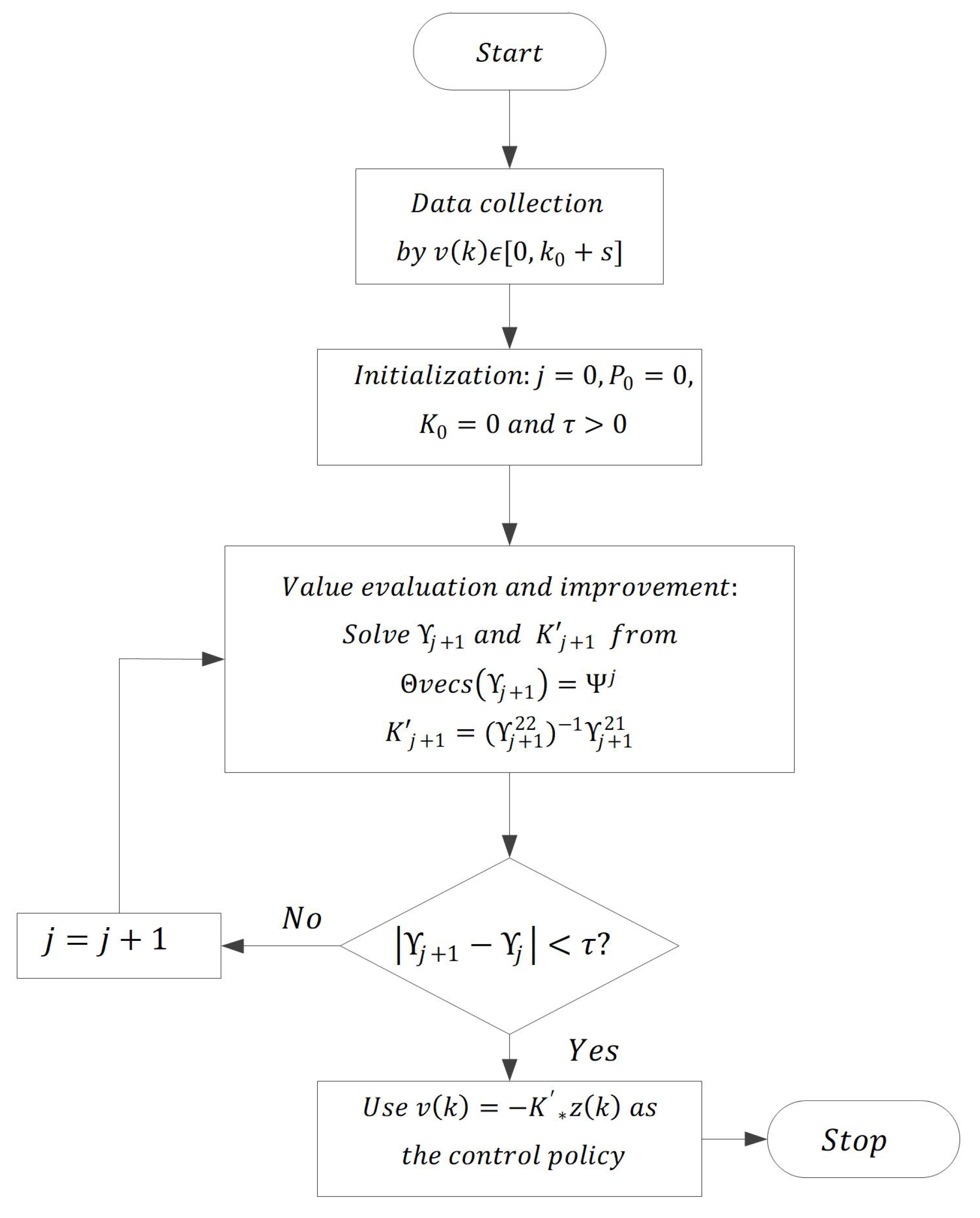
Hence, Algorithm 2 converges, and the closed-loop system is stable. The VI-based measurement feedback ADP flowchart is shown in Figure 2.
Algorithm 2ADP algorithm by the VI method.
1. Select an error τ > 0 and j = 0 .
2. Calculate K j :
Θ v e c s ( Y j + 1 ) = Ψ j K j + 1 = ( Y j + 1 22 ) 1 Y j + 1 21
where Y j + 1 = E j + 1 F j + 1 F j + 1 T G j + 1
3. Until | Y j + 1 Y j | < τ
Get the approximated optimal control policy:
v ( k ) = K * z ( k )
Theorem 2.
The original system optimal controller is:
u ( k ) = v ( k ) + u * ( k )
where u * ( k ) = K ¯ * z ¯ ( k ) and z ¯ ( k ) = η ˜ ( k 1 , k q ) u * ˜ ( k 1 , k q ) σ ˜ ( k 1 , k q ) . The proof is in Appendix D.
The optimal feedback controller is:
u ( k ) = K * z ( k ) K ¯ * z ¯ ( k )

4. Simulations

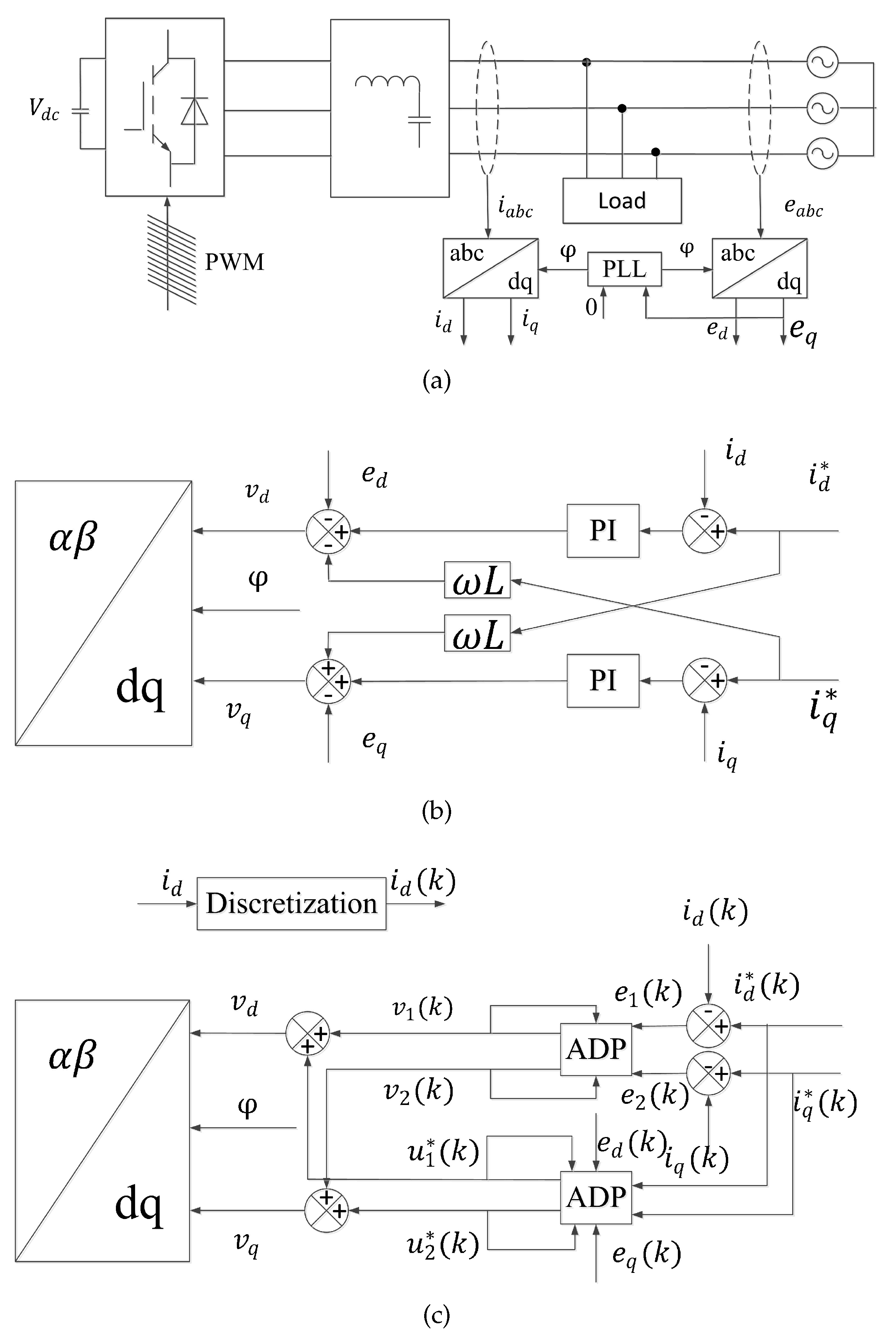
In this paper, r = 0.1 Ω , L = 1.5 mH, V d c = 1000 V, T s = 10 5 s, and Q = R = e y e ( 3 ) . Given i d * = 10 , i q * = 0 , and q = 1 , the inverter filter structure diagram and the comparison of the two control methods are shown in Figure 3. The inverter structure and d q component separation are shown in Figure 3a.
PI control is shown in Figure 3b. The PI regulation decoupling equation is:
v d = ( k P + k I s ) ( i d * i d ) w L i q * e d v q = ( k P + k I s ) ( i q * i q ) + w L i d * e q
where K p = 0.02 and K I = 500 [3]. ADP control is shown in Figure 3c. Calculate v and u * according to the current error and the command current, respectively. In Figure 3c, we can obtain ADP by Algorithm 1:
v d q ( k ) = K * e 12 ( k 1 ) v 12 ( k 1 ) K ¯ * i d q * ( k 1 ) u 12 * ( k 1 ) e d q ( k 1 )
where:
K * = 2.2762 0.0144 0.0153 0.0000 0.0144 2.2762 0.0000 0.0153
and:
K ¯ * = 2.2762 0.0144 0.0153 0.0000 0.0153 0.0000 0.0144 2.2762 0.0000 0.0153 0.0000 0.0153

4.1. Grid Voltage Balance

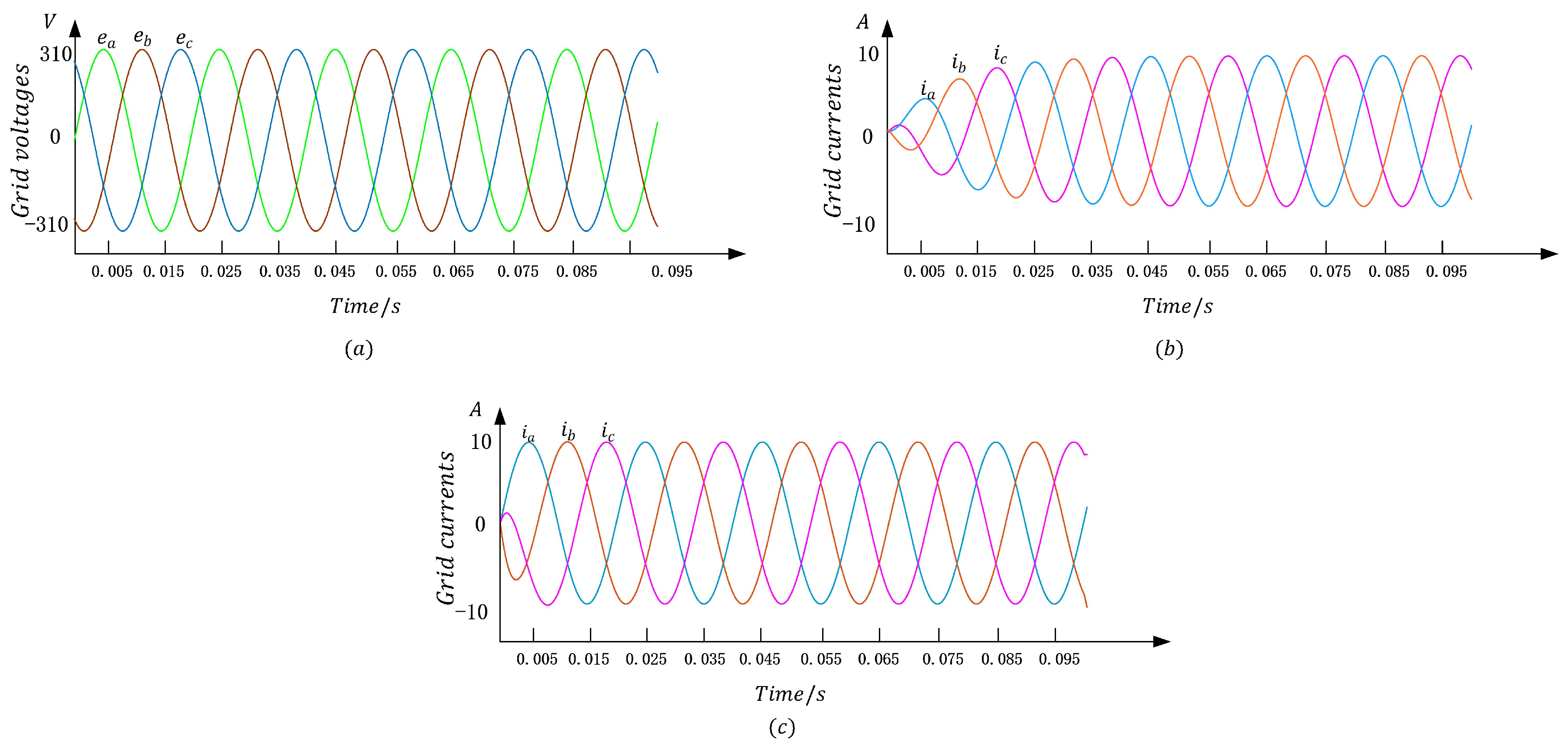
Grid voltage is shown in Figure 4a. It can be seen that the grid voltage is three-phase symmetrical with an amplitude of 310 V.
The grid current of PI closed-loop control and ADP closed-loop control is shown in Figure 4b,c, respectively. The figure shows in the case of grid voltage balance that the grid current tracking command value when the system reaches stability. From Figure 4b, we can see that the grid current reaches the steady state value at t = 0.005 s. From Figure 4c, we can see that the grid current reaches the steady state value at t = 0.035 s. This shows that the grid current of ADP closed-loop approach had a faster response speed than the PI closed-loop approach.

4.2. Grid Voltage Unbalance

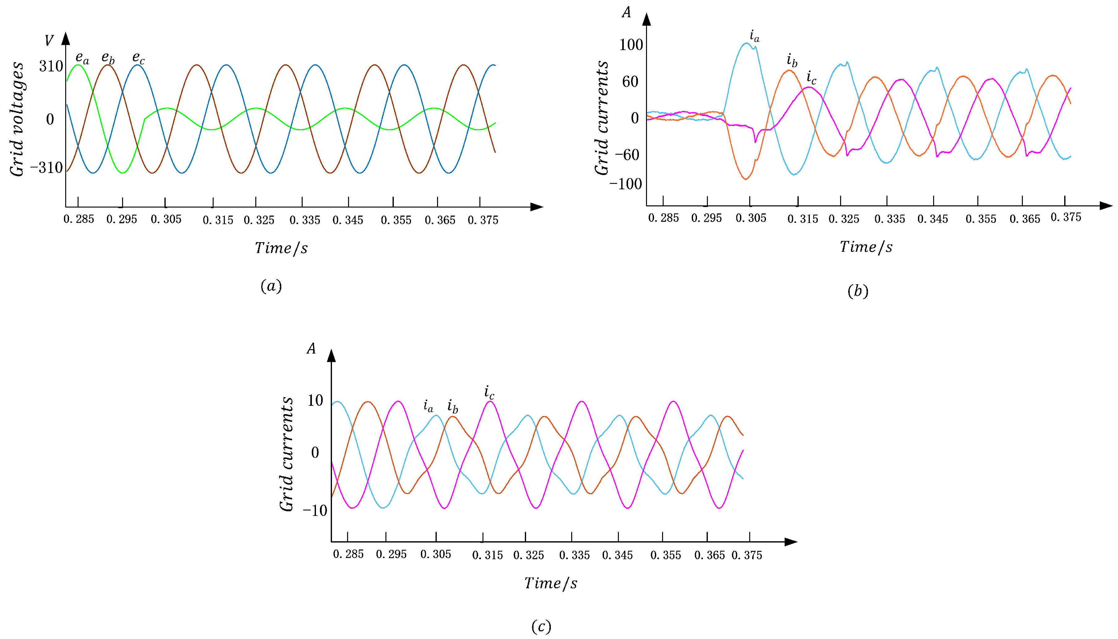
The grid voltage unbalance is shown in Figure 5a; at t = 0.3 s, the amplitude of the phase A voltage dropped by 80%.
The grid current of the PI closed-loop approach and the ADP closed-loop approach is shown in Figure 5b,c, respectively. As shown in Figure 5b, after the Phase A voltage dropped, the Phase A current rose sharply, and the highest amplitude reached 100 A. The Phase B and C currents also rose and finally stabilized at about 60 A. The current increased several times compared to the normal operation, which can damage the entire system. As shown in Figure 5c, after the Phase A voltage dropped, the phase A current saw almost no change, and the Phase B and C currents were reduced.

4.3. Grid Current Balance Control

The grid voltage unbalance had positive and negative sequence components. Therefore, the positive and negative sequence components should be controlled separately. To suppress the negative sequence components, the current command is:
i d * + = 10 i q * + = 0 i d * = 0 i q * = 0
By (9) and (10), positive and negative sequence component control had the same mathematical model. Therefore, the positive and negative sequences had the same control loop. By (35), the positive and negative sequence PI adjustment decoupling equations are:
v d + = ( k P + k I s ) ( i d + i d + ) w L i q + e d + v q + = ( k P + k I s ) ( i q + i q + ) + w L i d + e q +
and:
v d = ( k P + k I s ) ( i d i d ) w L i q e d v q = ( k P + k I s ) ( i q i q ) + w L i d e q
Then, negative and positive sequences had the same control process. By (5) and (6), the output voltage of the inverter is:
v d q = e j w t v d q + + e j w t v d q
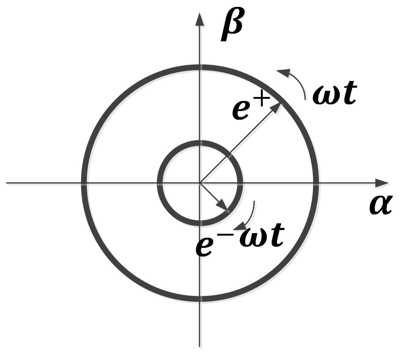
In this paper, the positive and negative sequence components were separated by modulus detection. By (6), in the α β coordinate system, the grid voltage positive sequence vector modulo | e + | , the angular frequency w rotated counterclockwise, the grid voltage negative sequence vector modulo | e | , and angular frequency w rotated clockwise are shown in Figure 6.
Both had the same angular velocity and the opposite direction of rotation. | e | was the largest when two vectors were in the same direction, and | e | was the smallest when in the opposite direction.
m a x | e | = | e + | + | e | m i n | e | = | e + | | e |
The modulus of the positive and negative sequence components is:
| e + | = 1 2 ( m a x | e | + m i n | e | ) | e | = 1 2 ( m a x | e | m i n | e | )
We can get the positive and negative order d q components respectively:
e d + = | e + | c o s φ e q + = | e + | s i n φ
and:
e d = | e | c o s φ e q = | e | s i n φ
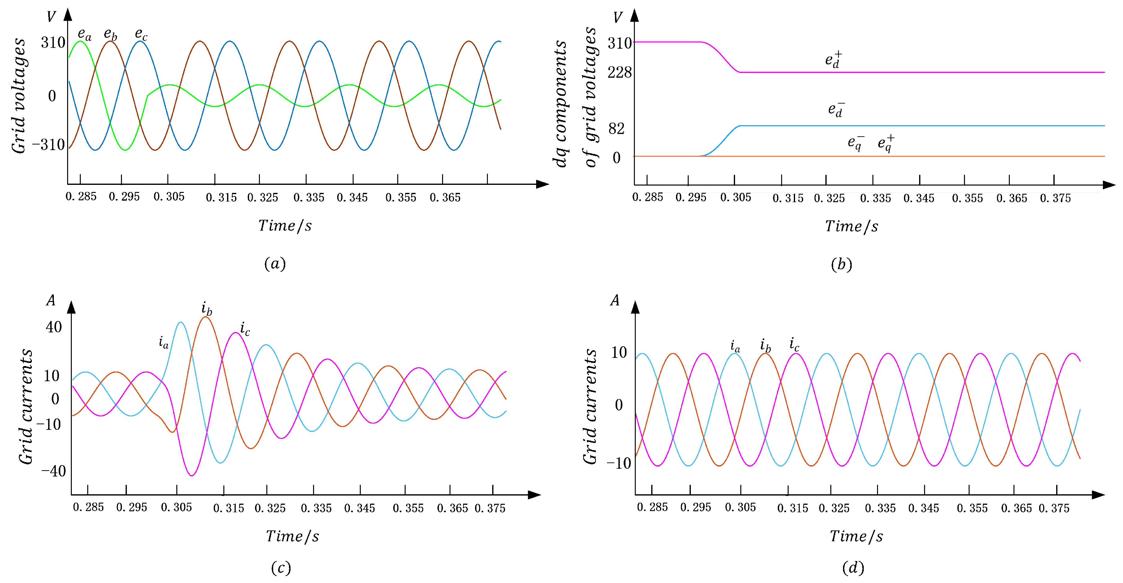
The grid voltage unbalance is shown in Figure 7a; at t = 0.3 s, the amplitude of the Phase A voltage dropped by 80%.
The grid voltage d q axis positive and negative sequence components are shown in Figure 7b.
The grid current of PI closed-loop control and ADP closed-loop control is shown in Figure 7c,d, respectively. As shown in Figure 7c, after the Phase A voltage dropped, the grid currents increased instantaneously, and the maximum was 40 A. After a brief rise, the current gradually approached stability, and when t = 0.345 s, the grid currents were stable. As shown in Figure 7d, after the Phase A voltage dropped, the grid current had almost no fluctuations in this process, keeping the command value. From this, we can see that the balanced current strategy using ADP closed-loop control not only could suppress the sharp rise of current, but also made the current respond quickly to the steady state value. The current overshoot of two control methods is shown in Table 1. Under PI closed-loop control, O v e r s h o o t ( A ) < 40 10 10 = 300 % , O v e r s h o o t ( B ) = 40 10 10 = 300 % , and O v e r s h o o t ( C ) < 40 + 10 10 = 300 % . Under the ADP closed-loop control, the grid currents were not overshot.

4.4. Grid Current Balance Control of Command Power

By [34], the command current calculation formula is:
i α β * = 2 3 1 e + e [ ( p * j q * ) e + e j w t ( p * + j q * ) e e j w t ]
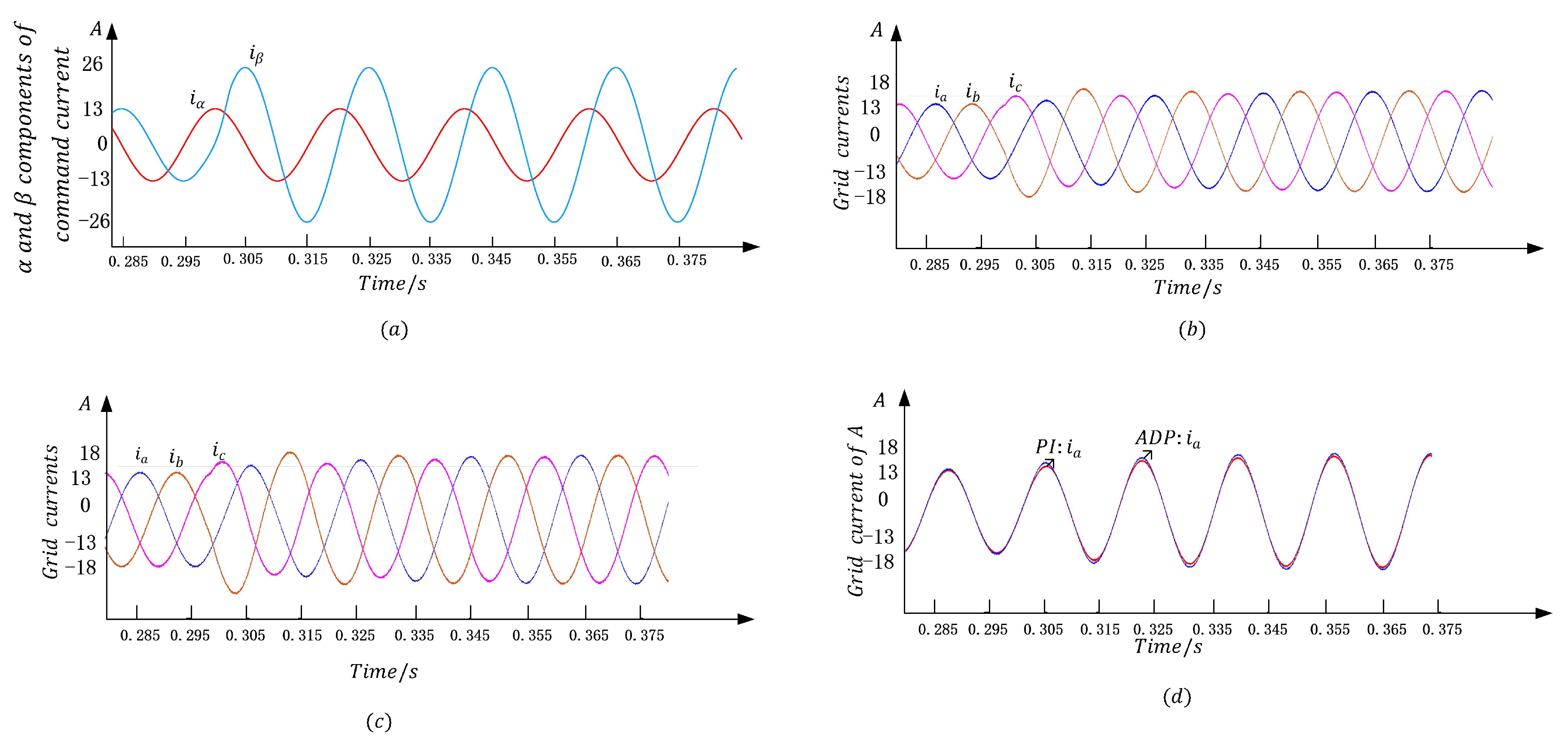
In this paper, we assumed p * = 6000 W and q * = 2000 W . The command current α and β components are shown in Figure 8a. The grid currents of PI closed-loop control and ADP closed-loop control are shown in Figure 8b,c, respectively. We can see that both control methods stabilized the current. Two control methods’ Phase A current comparison is shown in Figure 8d. We can see that the current of the ADP closed-loop control method was smoother at steady state. The T H D of grid currents are shown in Table 2. We can see that the three-phase grid currents T H D P I were 2.04 % , 1.87 % , and 1.97 % , and T H D A D P were 1.30 % , 1.29 % , 1.29 % . This shows that the ADP closed-loop control method had better steady state performance.

4.5. Discussions

The main purpose of this paper is to introduce the application of adaptive dynamic programming in grid-connected inverters. The simulation experiment was performed in the MATLAB/Simulink environment. Although the verification was for the Phase A voltage drop of 80 % , this can be verified for other situations.

5. Conclusions

In this paper, an ADP algorithm was proposed instead of the original PI algorithm. The optimal tracking problem was solved without the complete system mathematical model. In the control strategy proposed in this paper, the grid currents can track the command currents. Compared with PI closed-loop control, ADP closed-loop control reduces current oscillation and improved response speed.
In this paper, we only considered current as the indicator. However, in the actual microgrid system, there are many indicators that affect system performance. In the hierarchical droop-based control strategies [35,36], we can set different performance indicators under different requirements, such as P , Q ( P = P P * , and P and P * represent output active power and command active power, respectively. Q = Q Q * , and Q and Q * represent output reactive power and command reactive power, respectively). In island mode, we can set w and U ( w = w w * , and w and w * represent the output angular frequency and the given angular frequency, respectively. U = U U * , and U and U * represent the output voltage and the given voltage, respectively) as performance indicators. Then, we can set the performance indicator function according to the selected indicators and find the optimal controller by the ADP approach. This reduces system oscillations and improves performance.

Author Contributions

Y.Y., Z.W., and X.W. proposed the idea. Y.Y., Z.W., and X.W. built the MATLAB/Simulink simulation platform. Z.W. wrote the first draft of the manuscript. All authors contributed to and have approved the final manuscript.

Funding

This work was supported in part by the National Science Foundation of China (NSFC: 61563034) and the International S & T Cooperation Program of China (ISTCP:2014DFG72240).

Conflicts of Interest

The authors declare no conflict of interest.

Abbreviations

Variables
S k Switching variable
u k Inverter output voltage
i k Grid current
i d q Grid current dq-axis component
i d q + Grid current positive sequence dq-axis component
i d q Grid current negative sequence dq-axis component
e k Grid voltage
e d q Grid voltage dq-axis component
e d q + Grid voltage positive sequence dq-axis component
e d q Grid voltage negative sequence dq-axis component
φ Angle between the d-axis and the α -axis
wAngular frequency
J e ( k ) Performance
PSolution of ARE
KError system feedback control gain
e ( k ) Current error
v ( k ) Error system optimal controller
u * ( k ) Reference control track
u ( k ) Original system controller
K * Error system optimal feedback control gain
K ¯ * Original system optimal feedback control gain
Acronyms
PIProportional integral
A D P Adaptive dynamic programming
P I Policy iteration
V I Value iteration
L Q R Linear quadratic regulator
A R E Algebra Riccati equation
D T Discrete-time
Constants
rFilter resistor
LFilter inductor
V d c DC side voltage
T s Sampling period
QState error weighting matrix
RControl error weighting matrix
qNumber of online datasets
i d q * Command current dq-axis component
i d q + Command current positive sequence dq-axis component
i d q Command current negative sequence dq-axis component
K P Proportional parameter
K I Integral parameter

Appendix A

Proof. 
For a linear discrete system:
x ( k + 1 ) = G x ( k ) + H u ( k )
where x is an n-dimensional state vector and u is an n-dimensional input vector. By (A1), we can obtain:
x ( k ) = G k x ( 0 ) + i = 0 k 1 G k 1 i H u ( i )
We assume x ( n ) = 0 when k = n , then:
x ( 0 ) = i = 0 n 1 G 1 i H u ( i ) = [ G 1 H u ( 0 ) + G 2 H u ( 1 ) + + G n H u ( n 1 ) ] = S u ( 0 ) u ( 1 ) u ( n 1 )
where S = G 1 H G 2 H G n H R n * 2 n . For any initial value x ( 0 ) , the necessary and sufficient condition for the solution of Equation (A3) is:
r a n k ( S ) = n
In this paper, r = 0.1   Ω , L = 1.5 mH, w = 314 rad/s, A = r L w w r L , B = 1 L 0 0 1 L , G = T A + I , and H = T B . Then:
x ( k + 1 ) = G x ( k ) + H u ( k ) = 0 . 9993 0 . 0031 0 . 0031 0 . 9993 x ( k ) + 0 . 0067 0 0 0 . 0067 u ( k )
Then:
S = G 1 H G 2 H = 0 . 0067 0 0 . 0067 0 0 0 . 0067 0 0 . 0067
r a n k ( S ) = 2
The proof is thus complete. □

Appendix B

Proof. 
For a matrix A B K 0 , let us assume that it has n unequal eigenvalues, which are λ 1 , λ 2 , λ 3 , , λ n . The feature matrix of A B K 0 is T . We have:
e ( k ) = ( A B K 0 ) k e ( 0 ) = ( T λ 1 λ 2 λ n T 1 ) k e ( 0 ) = T λ 1 k λ 2 k λ n k T 1 e ( 0 )
Since T , e ( 0 ) are bounded and | λ i | < 1 . Then, k , and we have | λ i | k 0 and e ( k ) 0 . If matrix A B K 0 has heavy roots, we have the same proof. □

Appendix C

Proof of Theorem 1.
By (15), (18), and (21):
P = k = 0 ( A B K ) T k ( Q + K T R K ) ( A B K ) k
When j = 0 , by (22) and (A9), we have:
P 0 P 1 = k = 0 A 1 T k ( K 0 K 1 ) T R ( K 0 K 1 ) A 1 k 0
where A j = ( A B K j ) k . Then, by (19) and (A9), we obtain:
P 1 P * = k = 0 A 1 T k ( K 1 K * ) T R ( K 1 K * ) A 1 k 0
Therefore, we have P 0 P 1 P * . For j = 0 , 1 , , we can obtain that P j is the existence of a unique value. The proof is thus complete. □

Appendix D

Proof of Theorem 2.
By (12), (24), and (25), we can obtain:
η ( k ) = M ¯ z ¯ ( k ) = M e M v M σ z ¯ ( k )
where M σ = D q A q C q + T q and D q = D A D A q 1 D .
The ideal control system and error control system have the same coefficient matrices A and B. According to the above calculation process, we have:
K ¯ j = K j M e M v M σ = G ¯ F ¯ T

References

  1. Fei, L.; Yan, Z.; Duan, S.; Yin, J.; Liu, B.; Liu, F. Parameter Design of a Two-Current-Loop Controller Used in a Grid-Connected Inverter System With LCL Filter. IEEE Trans. Ind. Electron. 2009, 56, 4483–4491. [Google Scholar]
  2. Choi, U.M.; Lee, J.S.; Lee, K.B. New Modulation Strategy to Balance the Neutral-Point Voltage for Three-Level Neutral-Clamped Inverter Systems. IEEE Trans. Energy Convers. 2014, 29, 91–100. [Google Scholar] [CrossRef]
  3. Bayhan, S.; Kukrer, O.; Komurcugil, H. Model-Based Current Control Strategy with Virtual Time Constant for Improved Dynamic Response of Three-Phase Grid-Connected VSI. IEEE Trans. Ind. Electron. 2018, 66, 4156–4165. [Google Scholar]
  4. Gao, Y.G.; Jiang, F.Y.; Song, J.C.; Zheng, L.J.; Tian, F.Y.; Geng, P.L. A novel dual closed-loop control scheme based on repetitive control for grid-connected inverters with an LCL filter. ISA Trans. 2018, 74, 194–208. [Google Scholar] [CrossRef] [PubMed]
  5. Ikehara, Y.; Arai, K.; Furukawa, N. Improved control strategy with grid-voltage feedforward for LCL-filter-based inverter connected to weak grid. IET Power Electron. 2014, 7, 2660–2671. [Google Scholar]
  6. Tan, G.; Jie, C.; Sun, X. Tan-Sun Coordinate Transformation System Theory and Applications for Three-Phase Unbalanced Power Systems. IEEE Trans. Power Electron. 2017, 32, 7352–7380. [Google Scholar] [CrossRef]
  7. Mirabbasi, S.; Martin, K. Design of loop filter in phase-locked loops. Electron. Lett. 2002, 35, 1801–1802. [Google Scholar] [CrossRef]
  8. Robles, E.; Ceballos, S.; Pou, J.; Martín, J.L.; Zaragoza, J.; Ibañez, P. Variable-Frequency Grid-Sequence Detector Based on a Quasi-Ideal Low-Pass Filter Stage and a Phase-Locked Loop. IEEE Trans. Power Electron. 2010, 25, 2552–2563. [Google Scholar] [CrossRef]
  9. Baghaee, H.R.; Mirsalim, M.; Gharehpetian, G.B.; Talebi, H.A. Three-phase AC/DC power-flow for balanced/unbalanced microgrids including wind/solar, droop-controlled and electronically-coupled distributed energy resources using radial basis function neural networks. IET Power Electron. 2018, 10, 313–328. [Google Scholar] [CrossRef]
  10. Baghaee, H.R.; Mirsalim, M.; Gharehpetian, G.B.; Talebi, H.A. A generalized descriptor-system robust H control of autonomous microgrids to improve small and large signal stability considering communication delays and load nonlinearities. Int. J. Electr. Power Energy Syst. 2018, 92, 63–82. [Google Scholar] [CrossRef]
  11. Kamihigashi, T. Elementary Results on Solutions to the Bellman Equation of Dynamic Programming: Existence, Uniqueness, and Convergence. Econ. Theory 2014, 56, 251–273. [Google Scholar] [CrossRef]
  12. Zhao, H.B.; Wang, B.Y.; Liao, J.X.; Wang, H.K.; Tan, G. Adaptive Dynamic Programming for Control: Algorithms and Stability. Commun. Control Eng. 2013, 54, 6019–6022. [Google Scholar]
  13. Gao, W.; Jiang, Z.P. Adaptive dynamic programming and adaptive optimal output regulation of linear systems. IEEE Trans. Autom. Control 2016, 62, 4164–4169. [Google Scholar] [CrossRef]
  14. Jiang, Y.; Jiang, Z.P. Robust Adaptive Dynamic Programming With an Application to Power Systems. IEEE Trans. Neural Networks Learn. Syst. 2013, 24, 1150–1156. [Google Scholar] [CrossRef] [PubMed]
  15. Liu, D.R.; Wang, D.; Zhao, D.B.; Wei, Q.L.; Jin, N. Neural-Network-Based Optimal Control for a Class of Unknown Discrete-Time Nonlinear Systems Using Globalized Dual Heuristic Programming. IEEE Trans. Autom. Sci. Eng. 2012, 9, 628–634. [Google Scholar] [CrossRef]
  16. Jiang, Y.; Jiang, Z.P. Computational adaptive optimal control for continuous-time linear systems with completely unknown dynamics. Automatic 2012, 48, 2699–2704. [Google Scholar] [CrossRef]
  17. Jiang, Y.; Jiang, Z.P. Adaptive dynamic programming as a theory of sensorimotor control. Biol. Cybern. 2014, 108, 459–473. [Google Scholar] [CrossRef]
  18. Jiang, Y.; Jiang, Z.P. Global Adaptive Dynamic Programming for Continuous-Time Nonlinear Systems. IEEE Trans. Autom. Control 2015, 60, 2917–2929. [Google Scholar] [CrossRef] [Green Version]
  19. Vrabie, D.; Pastravanu, O.; Abu-Khalaf, M.; Lewis, F.L. Brief paper: Adaptive optimal control for continuous-time linear systems based on policy iteration. Automatic 2009, 45, 477–484. [Google Scholar] [CrossRef]
  20. Wang, F.Y.; Jin, N.; Liu, D.R.; Wei, Q.L. Adaptive dynamic programming for finite-horizon optimal control of discrete-time nonlinear systems with ε-error bound. IEEE Trans. Neural Netw. 2011, 22, 24–36. [Google Scholar] [CrossRef]
  21. Wei, Q.L.; Liu, D.R.; Lin, H. Value Iteration Adaptive Dynamic Programming for Optimal Control of Discrete-Time Nonlinear Systems. IEEE Trans. Cybern. 2016, 46, 840–853. [Google Scholar] [CrossRef] [PubMed]
  22. Bian, T.; Jiang, Z.P. Value iteration and adaptive dynamic programming for data-driven adaptive optimal control design. Automatic 2016, 71, 348–360. [Google Scholar] [CrossRef] [Green Version]
  23. Huang, M.Z.; Gao, W.N.; Jiang, Z.P. Connected cruise control with delayed feedback and disturbance: An adaptive dynamic programming approach. Int. J. Adapt. Control Signal Process. 2017, 6, 356–370. [Google Scholar] [CrossRef]
  24. Johnson, C. Accomodation of external disturbances in linear regulator and servomechanism problems. IEEE Trans. Autom. Control 1971, 16, 635–644. [Google Scholar] [CrossRef]
  25. Saberi, A.; Stoorvogel, A.; Sannuti, P. On output regulation for linear systems. Int. J. Control 2001, 74, 783–810. [Google Scholar] [CrossRef]
  26. De Santis, R.; Isidori, A. On the output regulation for linear systems in the presence of input saturation. IEEE Trans. Autom. Control 2001, 46, 156–160. [Google Scholar] [CrossRef]
  27. Zhang, H.G.; Wei, Q.L.; Luo, Y.H. A novel infinite-time optimal tracking control scheme for a class of discrete-time nonlinear systems via the greedy HDP iteration algorithm. IEee Trans. Syst. Man Cybern. Part B 2008, 38, 937–942. [Google Scholar] [CrossRef] [PubMed]
  28. Park, Y.M.; Choi, M.S.; Lee, K.Y. An optimal tracking neuro-controller for nonlinear dynamic systems. IEEE Trans. Neural Netw. 1996, 7, 1009–1110. [Google Scholar]
  29. Athans, M. On the design of PID controllers using optimal linear regulator theory. Automatic 1971, 7, 643–647. [Google Scholar] [CrossRef]
  30. Kleinman, D. On an iterative technique for Riccati equation computations. IEEE Trans. Autom. Control 1968, 13, 114–115. [Google Scholar] [CrossRef]
  31. Bian, T.; Jiang, Y.; Jiang, Z.P. Decentralized Adaptive Optimal Control of Large-Scale Systems With Application to Power Systems. IEEE Trans. Ind. Electron. 2015, 62, 2439–2477. [Google Scholar] [CrossRef]
  32. Choeung, C.; Kry, M.L.; Lee, Y.I. Robust Tracking Control of a Three-Phase Charger under Unbalanced Grid Conditions. Energies 2018, 11, 3389. [Google Scholar] [CrossRef]
  33. Gao, W.N.; Jiang, Z.P. Adaptive Optimal Output Regulation of Discrete-time Linear Systems subject to Input Time-delay. In Proceedings of the Annual American Control Conference, Milwaukee, WI, USA, 27–29 June 2018; pp. 4484–4489. [Google Scholar]
  34. Valouch, V.; Bejvl, M.; Simek, P.; Skramlik, J. Power Control of Grid-Connected Converters Under Unbalanced Voltage Conditions. IEEE Trans. Ind. Electron. 2015, 62, 4241–4248. [Google Scholar] [CrossRef]
  35. Guerrero, J.M.; Vasquez, J.C.; Matas, J.; De Vicuña, L.G.; Castilla, M. Hierarchical Control of Droop-Controlled AC and DC Microgrids—A General Approach Toward Standardization. IEEE Trans. Ind. Electron. 2011, 58, 158–172. [Google Scholar] [CrossRef]
  36. Baghaee, H.R.; Mirsalim, M.; Gharehpetian, G.B. Gharehpetian. Performance improvement of Multi-DER microgrid for small and large-signal disturbances and nonlinear loads: novel complementary control loop and fuzzy controller in a hierarchical droop-based control scheme. IEEE Syst. J. 2018, 12, 444–451. [Google Scholar] [CrossRef]
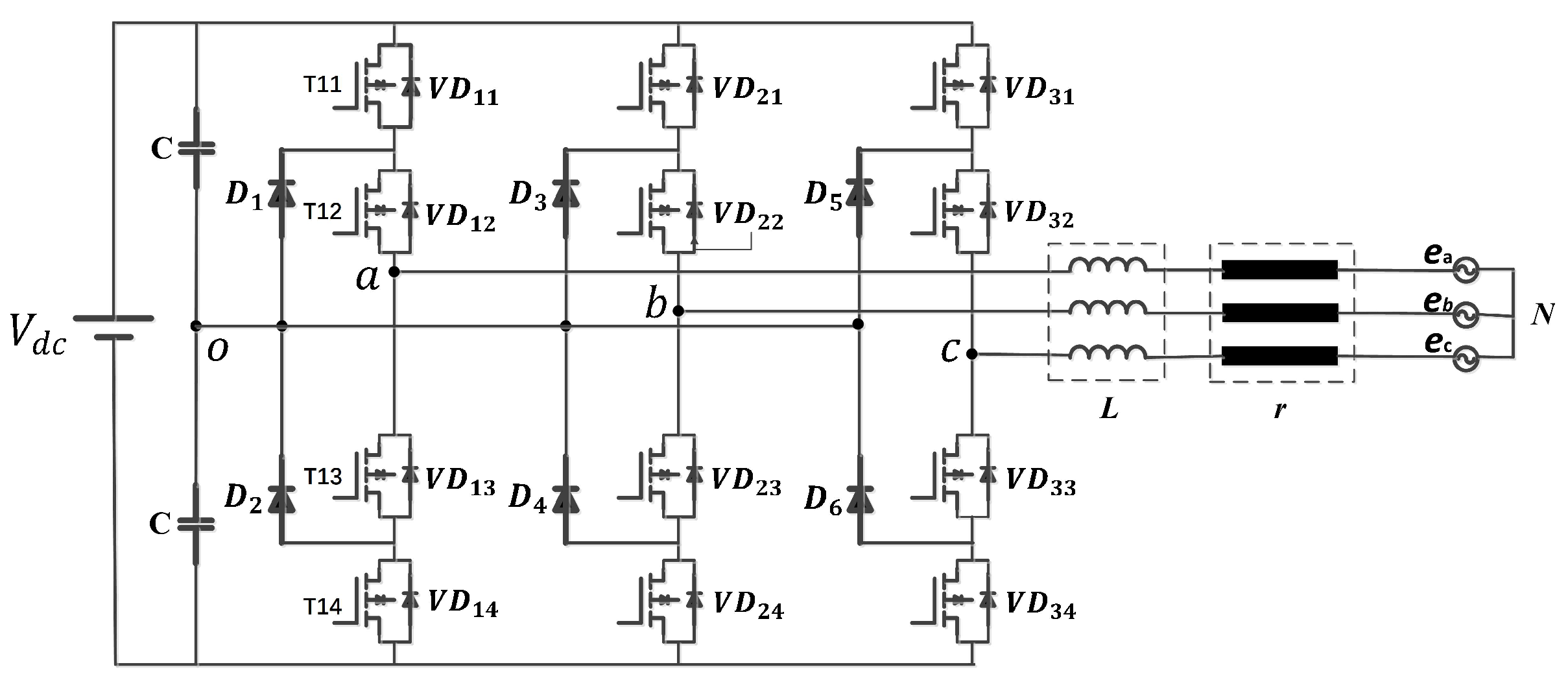
Figure 1. Three-level inverter topology.
Energies 12 02864 g001
Figure 2. ADP algorithm by the VI method flowchart.
Energies 12 02864 g002
Figure 3. Inverter block diagram (a). PI closed-loop control block diagram (b). ADP closed-loop control block diagram (c).
Energies 12 02864 g003
Figure 4. Grid voltages (a). Grid currents of PI closed-loop control (b). Grid currents of ADP closed-loop control (c).
Energies 12 02864 g004
Figure 5. Grid voltages (a). Grid currents of PI closed-loop control (b). Grid currents of ADP closed-loop control (c).
Energies 12 02864 g005
Figure 6. Schematic diagram of the positive and negative sequence α β coordinate system of the grid voltage.
Energies 12 02864 g006
Figure 7. Grid voltages (a). Positive and negative sequence d q component of grid voltages (b). Grid currents of PI closed-loop control (c). Grid currents of ADP closed-loop control (d).
Energies 12 02864 g007
Figure 8. α and β components of command currents (a). Grid currents of PI closed-loop control (b). Grid currents of ADP closed-loop control (c). Two control methods’s Phase A current comparison (d).
Energies 12 02864 g008
Table 1. Overshoot of grid currents.
Control MethodPhase A CurrentPhase B CurrentPhase C Current
PI closed loop control<300%300%−300%
ADP closed loop controlNo overshootNo overshootNo overshoot
Table 2. THD of grid currents.
Control MethodPhase A CurrentPhase B CurrentPhase C Current
PI closed-loop control2.04%1.87%1.97%
ADP closed-loop control1.30%1.29%1.29%