Determining the Responsibility of Three-Phase Unbalanced Sources Based on RICA

Abstract

Voltage unbalance is one of the main power quality problems, and the source of many negative effects on utilities that are experienced by customers. In this paper, a method based on robust independent component analysis (RICA) for responsibility division of unbalanced sources is proposed for voltage unbalance. According to the weak correlation between negative-sequence voltage and upstream and downstream current fluctuation at the point of common coupling (PCC), the independent component of the negative-sequence voltage and current fluctuation at the point of common coupling is obtained by RICA. The blind source mixing coefficient matrix can be obtained according to the least squares method. The equivalent negative-sequence impedance on both sides of the PCC can be obtained using the linear correlation between the mixing coefficients. Finally, according to the principle of partial pressure, the unbalance contribution of the upstream and downstream at the PCC is calculated. The method is accurate for upstream and downstream impedance estimation compared with the traditional method, and has a strong anti-interference ability. When the background noise or system fluctuation is large, the responsibility division result is still accurate. The correctness and effectiveness of the proposed method are proven by the simulation of the experimental circuit.

1. Introduction

With the deepening of reform, electric retail companies will enhance their competitiveness by improving service levels, providing value-added services and better-quality power. As one of the main power-quality problems, voltage unbalance has caused widespread concern among power sellers and consumers [1,2,3,4]. Voltage unbalance refers to the phenomenon that the voltage amplitude of the fundamental frequency is not equal, or that the phase is offset in a three-phase power system [5,6]. In a power system, voltage unbalance is the result of a combination of numerous unbalanced sources. Unusual access or operation of sources, lines, and loads can cause voltage unbalance, such as single-phase ground faults, wire break resonance, single-phase load access, asymmetrical wiring distribution of transformers, and so on [1]. Voltage unbalance has many negative effects on distribution networks and customers. For example, transmission line losses increase and grid operations overheat, reducing operating efficiency and equipment life, and increasing equipment maintenance costs. 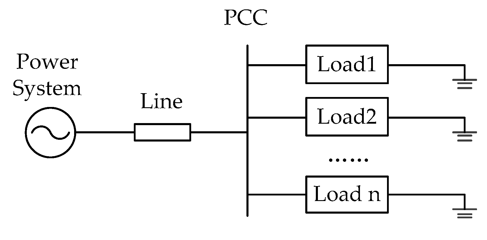In 2008, the International Electro-Technical Commission released regulations about the limits of unbalanced loads accessing high voltage, medium voltage and low voltage systems [7]. When an unbalance at the point of common coupling (PCC) exceeds the standard in a power system, the unbalanced source needs to be located and the penalties should be quantified that grid companies and customers should be exposed to by unbalanced responsibility division calculations.

At present, the research on voltage unbalance mainly focuses on the division of unbalanced responsibility, unbalanced source location, calculation of node unbalance [1,2,3,4,5,6,7,8,9,10,11,12,13,14,15], and research on voltage unbalance mitigation measures. The assessment of the contribution of unbalanced sources at the point of common coupling is the premise of responsibility division and governance. Mahyar Abasi proposed to establish a model in the n-node radial distribution network to analyze the impact of loads, lines, and sources on the system unbalance, but the topology of the system needs to be known [4]. According to circuit topology, Sun Yuanyuan has derived the general formula for the division of unbalanced sources responsibility, which only requires knowledge of the voltage and current at the PCC [5,6]. In [8], the three-phase power flow method was used to evaluate the effects of unbalanced sources and loads on the unbalance factor. In [9], the three traditional methods of IEC (International Electrotechnical Commission)—three-phase power flow, and the conforming and nonconforming current methods—are used to calculate the effect of unbalanced sources responsibility division, and the advantages and disadvantages of each method are discussed. Milanovic calculated the range of voltage unbalance factor by Monte Carlo simulation, and estimated the unbalance from historical data even where the test data were missing [10]. A method has also been proposed to improve the computational efficiency of unbalance factor by transforming the square root operation into a trigonometric equation of geometry, then approximating the trigonometric equation by algebraic operations [11]. Jayatunga proposed deterministic methodologies to assess constituent components of postconnection voltage unbalance levels at the point of evaluation in interconnected and radial networks [12,13]. The above scholars have provided many methods for the calculation of unbalance factors and contribution determination, but there are still many shortcomings.

In view of the shortcomings of the above literature, this paper proposes a method based on robust independent component analysis (RICA) for unbalanced sources responsibility division. According to the weak correlation between the negative-sequence voltage and the current fluctuation of upstream and downstream at the point of common coupling, the independent component of the negative-sequence voltage and current fluctuation could be obtained by RICA. The blind source mixing coefficient matrix can be obtained according to the least squares method. The equivalent negative-sequence impedance on both sides can be calculated by using the linear correlation between the mixing coefficients. Finally, according to the principle of partial pressure, the unbalance contribution of the upstream and downstream at the PCC could be obtained. Determined through simulation experiments, the estimated value of system impedance and the result of responsibility division calculated by the method proposed in this paper were more accurate than traditional methods. At the same time, the method had a strong anti-interference ability, and system noise and fluctuation had little influence over the result error.

The main contents of the paper are summarized as follows. In Section 2, the unbalanced source equivalent model is established and a responsibility division index is proposed. In Section 3, the equivalent current source and equivalent impedance are solved using RICA and a least squares method, then dividing the unbalanced responsibility. The calculation steps are summarized in Section 4. The simulation and field data analysis results are given in Section 5. The conclusion is summarized in Section 6.

2. Unbalanced Source Equivalent Analysis Model

2.1. Voltage Unbalance Factor

Three-phase unbalance is one of the main problems with power quality. Voltage unbalance factor (VUF) is a commonly used indicator for quantifying the severity of unbalances, and is usually calculated by dividing the negative-sequence voltage or current by the positive-sequence voltage or current [14], as shown in Equations (1) and (2).

$$VU{F}_U=\frac{U_{negative}}{U_{positive}}\times 100\%$$

(1)

$$VU{F}_I=\frac{I_{negative}}{I_{positive}}\times 100\%$$

(2)

where U_negative is the negative-sequence voltage rms, and U_positive is the positive-sequence voltage rms. I_negative and I_positive are the negative-sequence and positive-sequence current rms, respectively.

In EN 50160 [15], it is stipulated that 95% of the average voltage unbalance factors in 10 min cannot exceed 2% in one week in LV (low voltage) and MV (medium voltage) networks, and cannot exceed 1% in one week in HV (high voltage) networks. As shown in Figure 1, the power-in end of the important customer is a measurement point, and the system side on the left of the PCC is referred to as the upstream, while the customer load on the right side of the PCC is referred to as the downstream. The unbalance sources of upstream include uneven line impedance and other load impedance unbalances in the system. The unbalance sources of downstream include single-phase loads, dual-phase loads and three-phase unbalanced loads.

2.2. Unbalanced Source Equivalent Model

The influence of the upstream and downstream on the negative-sequence current at the PCC is equivalent to the negative-sequence Norton equivalent circuit, as shown in Figure 2. Equation (3) is obtained from the Norton equivalent circuit:

$$\left[\begin{array}{c}\Delta U_{PCC2}\\ \Delta I_{PCC2}\end{array}\right]=\left[\begin{array}{cc}\frac{Z_{U2}{Z}_{D2}}{Z_{D2}+Z_{U2}}& \frac{Z_{U2}{Z}_{D2}}{Z_{D2}+Z_{U2}}\\ \frac{Z_{D2}}{Z_{D2}+Z_{U2}}& -\frac{Z_{U2}}{Z_{D2}+Z_{U2}}\end{array}\right]\left[\begin{array}{c}\Delta I_{D2}\\ \Delta I_{U2}\end{array}\right]$$

(3)

where $\Delta$I_U2 and $\Delta$I_L2 are the equivalent negative-sequence current source-fluctuation vector values of the upstream and downstream, respectively; $\Delta$U_PCC2 and $\Delta$I_PCC2 are the negative-sequence voltage-fluctuation vector and negative-sequence current-fluctuation vectors of the PCC, respectively; and Z_U2 and Z_L2 are the equivalent negative-sequence impedance of the upstream and the downstream, respectively.

The real and imaginary parts of the Norton equivalent equation are separated and written in the plural form, which simplifies as Equation (4).

$$\left[\begin{array}{l}\Delta U_{PCC2,x}\hfill \\ \Delta U_{PCC2,y}\hfill \\ \Delta I_{PCC2,x}\hfill \\ \Delta I_{PCC2,y}\hfill \end{array}\right]=\left[\begin{array}{cccc}{a}_{11}& a_{12}& a_{13}& a_{14}\\ a_{21}& a_{22}& a_{23}& a_{24}\\ a_{31}& a_{32}& a_{33}& a_{34}\\ a_{41}& a_{42}& a_{43}& a_{44}\end{array}\right]\left[\begin{array}{c}\Delta I_{D2,x}\\ \Delta I_{D2,y}\\ \Delta I_{U2,x}\\ \Delta I_{U2,y}\end{array}\right]$$

(4)

where $\Delta$U_PCC2,x, $\Delta$U_PCC2,y, $\Delta$I_PCC2,x, and $\Delta$I_PCC2,y are the real and imaginary parts of the voltage and current vector fluctuations at the PCC; $\Delta$I_D2,x, $\Delta$I_D2,y, $\Delta$I_U2,x, and $\Delta$I_U2,y are the real and imaginary parts of the downstream and upstream current source vector fluctuations, respectively; a_ij (i, j = 1, 2, 3, 4) is the unbalanced current fluctuation coefficient and is only related to the equivalent impedance.

The three-phase current and voltage at the PCC can be obtained by measurement, and the collected information is subjected to Fourier analysis to obtain the fundamental frequency component of the voltage and current. By calculating the symmetrical component method, the phase component can be converted into the sequence component, as shown in Equations (5) and (6).

$$\left[\begin{array}{l}{\dot{U}}_1\\ {\dot{U}}_2\\ {\dot{U}}_0\end{array}\right]=\frac{1}{3}\left[\begin{array}{ccc}1& \alpha & {\alpha }^2\\ 1& {\alpha }^2& \alpha \\ 1& 1& 1\end{array}\right]\left[\begin{array}{l}{\dot{U}}_A\\ {\dot{U}}_B\\ {\dot{U}}_C\end{array}\right]$$

(5)

$$\left[\begin{array}{l}{\dot{I}}_1\\ {\dot{I}}_2\\ {\dot{I}}_0\end{array}\right]=\frac{1}{3}\left[\begin{array}{ccc}1& \alpha & {\alpha }^2\\ 1& {\alpha }^2& \alpha \\ 1& 1& 1\end{array}\right]\left[\begin{array}{l}{\dot{I}}_A\\ {\dot{I}}_B\\ {\dot{I}}_C\end{array}\right]$$

(6)

where $\alpha =e^{j2\pi /3}$, and ${\dot{U}}_A$, ${\dot{U}}_B$, ${\dot{U}}_C$ and ${\dot{I}}_A$, ${\dot{I}}_B$, ${\dot{I}}_C$ are the three-phase voltage and current, respectively.

When the unbalanced source on the upstream acts alone, the unbalanced negative-sequence voltage U_upstream2 generated at the PCC can be derived according to Ohm’s law:

$$U_{upstream2}=I_{U2}{Z}_{U2}\frac{Z_{U2}}{Z_{U2}+Z_{D2}}$$

(7)

Since the unbalanced voltage of the PCC is formed by the superposition of the upstream and downstream vector, the unbalanced negative-sequence voltage generated by the unbalanced downstream source acting alone at the PCC can be calculated according to Equation (8).

$$U_{downstream2}=U_{PCC2}-U_{upstream2}$$

(8)

The upstream and downstream contributions to the unbalanced negative-sequence voltage of PCC are shown in Figure 3. The indicator of unbalanced responsibility is shown in Equations (9) and (10).

$$F_{up}=\frac{\left|U_{upstream2}\right|\cos \delta }{\left|U_{PCC2}\right|}\times 100\%$$

(9)

$$F_{down}=\frac{\left|U_{downstream2}\right|\cos \beta }{\left|U_{PCC2}\right|}\times 100\%$$

(10)

If F_up is much larger than F_down, the upstream is the main source of unbalance. If F_down is much larger than F_up, the downstream is the main source of unbalance. The responsibilities of both sides can be obtained by F_up and F_down.

3. Unbalanced Responsibility Division Based on RICA Principle

3.1. RICA

Independent component analysis (ICA) was developed with the problem of blind source separation (BSS) [16], and finds optimal step sizes through a linear search. The mathematical model of ICA is

$$X(t)=AS(t)$$

(11)

where t (t = 1,2,…, t_n) is discrete time; S(t) is the source signal, and S(t) = [S₁(t), S₂(t),… , S_N(t)]^T; and X(t) is a matrix of observable signals, and X(t) = [X₁(t), X₂(t),…, X_M(t)]^T. Generally speaking, $M\ge N$. A is a mixing matrix that reflects the weight ratio of the source signal S(t) in the observed signal. Y = [y₁, y₂,…, y_N]^T is the estimator, and the signal vector Y is a reliable estimate of the source signal vector S, as shown in Equation (12):

$$Y(t)=WX(t)$$

(12)

Equation (13) can be obtained by combining Equation (11) with Equation (12):

$$Y(t)=WX(t)=WAS(t)=DS(t)$$

(13)

where D is a global matrix.

Scholars such as Zarzoso have proposed a high-efficiency calculation method for blind source separation [17,18,19,20]. The non-Gaussian properties of Y are often measured using kurtosis, the simple expression of which is

$$kurt(y)=E\{y^4\}-3{(E\{y^2\})}^2$$

(14)

where $E\{\cdot \}$ indicates mathematical expectation.

The purpose of RICA is to get the unmixing matrix W, and kurtosis is expressed as a function of the unmixed vector $\omega$:

$$K(\omega )=\frac{E\{{\left|y\right|}^4\}-2E^2\{{\left|y\right|}^2\}-{\left|E\{y^2\}\right|}^2}{E^2\{{\left|y\right|}^2\}}$$

(15)

At the same time, the same criteria as kurtosis can be expressed as a step polynomial or rational function. Using the exact linear search of the kurtosis absolute objective function, the global optimal step size μ_opt is determined by finding the root of the low-order polynomial. The expression is as follows:

$${\mu }_{opt}=\arg \underset{\mu }{\max }\left|K(\omega +\mu g)\right|$$

(16)

where the search direction g is usually a gradient, and $g={\nabla }_{\omega }K(\omega )$, as shown in Equation (17).

$${\nabla }_{\omega }{\rm K}(\omega )=\frac{4}{E^2\{{\left|y\right|}^2\}}\{E\{{\left|y\right|}^2{y}^{*}x\}-E\{yx\}E\{y^{*2}\}-\frac{(E\{{\left|y\right|}^4\}-{\left|E\{y^2\}\right|}^2)E\{y^{*}x\}}{E\{{\left|y\right|}^2\}}\}$$

(17)

Equation (15) is transformed into the function of $\mu$:

$$K(\mu )=\frac{E\{{\left|y^{+}\right|}^4\}-{\left|E\{{(y^{+})}^2\}\right|}^2}{E^2\{{\left|y^{+}\right|}^2\}}-2=\frac{p(\mu )}{Q^2(\mu )}-2$$

(18)

where y⁺ = y + μg, y = ω^Tx, g = g^Tx, p(μ) = p₁(μ)-|p₁(μ)|², Q(μ) = E(|y⁺|²), p₁(μ) = E(|y⁺|⁴), p₂(μ) = E(|y⁺|²).

Find the root ${\{{\mu }_l\}}_{l=1}^4$ of the step–size polynomial so that the absolute value of the objective function along the search direction is the largest:

$${\mu }_{opt}=\arg \underset{l}{\max }\left|K(\mathit{\omega }(k-1)+{\mu }_{l}g)\right|$$

(19)

Updating the unmixing matrix using the root of the step–size polynomial obtained:

$$\mathit{\omega }(k)=\mathit{\omega }(k-1)+{\mu }_{opt}g$$

(20)

In order to correct the ambiguity caused by scale invariance, the unmixing matrix needs to be normalized:

$${\mathit{\omega }}^{*}(k)=\frac{\mathit{\omega }(k)}{\Vert \mathit{\omega }(k)\Vert }$$

(21)

3.2. Unbalanced Responsibility Division based on RICA

As shown in Equation (22), Equation (4) is converted to the RICA standard matrix form:

$$X=AI$$

(22)

where the observation signal is X = [$\Delta$U_PCC2,x, $\Delta$U_PCC2,y, $\Delta$I_PCC2,x , $\Delta$I_PCC2,y]^T. The source signal is I = [$\Delta$I_D2,x, $\Delta$I_D2,y, $\Delta$I_U2,x , $\Delta$I_U2,y]^T, and A is the coefficient matrix. According to Equation (4), the observed signal ($\Delta$U_PCC2,x, $\Delta$U_PCC2,y, $\Delta$I_PCC2,x, and $\Delta$I_PCC2,y) is a linear combination of the source signals ($\Delta$I_D2,x, $\Delta$I_D2,y, $\Delta$I_U2,x, and $\Delta$I_U2,y). Four independent source signals I_j (j = 1, 2, 3, 4) can be obtained by unmixing the matrix X using RICA.

Assume that the relationship between the independent component I_j and the source signal after unmixing is:

$$\left[\begin{array}{c}{I}_1\\ I_2\\ I_3\\ I_4\end{array}\right]=\left[\begin{array}{c}{\beta }_1\Delta I_{D2,x}\\ {\beta }_2\Delta I_{D2,y}\\ {\beta }_3\Delta I_{U2,x}\\ {\beta }_4\Delta I_{U2,y}\end{array}\right]$$

(23)

where β_j (j = 1, 2, 3, 4) is a non-zero real number. Calculate the mixing coefficient P_i of I_j using the least squares method, as shown in Equation (24):

$$P_i=X_i{I}^{\mathrm{T}}{(I\cdot I^{\mathrm{T}})}^{-1}i=1,2,3,4$$

(24)

where $P_i$=${\left[p_{1i},p_{2i},p_{3i},p_{4i}\right]}^{\mathrm{T}}$.

The element p_ij in the mixing coefficient P_i has a proportional relationship with a_ij in Equation (4):

$$p_{ij}=\frac{a_{ij}}{{\beta }_j}\hspace{1em}i,j=1,2,3,4$$

(25)

Then,

$$\{\begin{array}{l}{p}_{1j}=p_{3j}{Z}_{S2,x}-p_{4j}{Z}_{S2,y}\\ p_{2j}=p_{3j}{Z}_{S2,y}+p_{4j}{Z}_{S2,x}\end{array}j=1,2$$

(26)

or

$$\{\begin{array}{l}{p}_{1j}=p_{3j}(-Z_{L2,x})-p_{4j}(-Z_{L2,y})\\ p_{2j}=p_{3j}(-Z_{L2,y})+p_{4j}(-Z_{L2,x})\end{array}j=3,4$$

(27)

The solution of Equations (26) and (27) are the same and can be derived as

$$\{\begin{array}{l}{Z}_{U2,x},-Z_{D2,x}=\frac{p_{1j}{p}_{3j}+p_{2j}{p}_{4j}}{p_{3j}^2+p_{4j}^2}\\ Z_{U2,y},-Z_{D2,y}=\frac{p_{2j}{p}_{3j}-p_{1j}{p}_{4j}}{p_{3j}^2+p_{4j}^2}\end{array}$$

(28)

The real part of the impedance in the system is mostly positive, and the upstream and downstream impedance can be judged according to the signs of Z_U2,x and Z_D2,x in Equation (28). Based on the Z_U2 and Z_D2 that have been solved, it is possible to calculate the negative-sequence voltages U_upstream2 and U_downstream2, as shown in Equations (7) and (8), respectively. Finally, the unbalanced contributions of upstream and downstream are calculated using Equations (9) and (10).

4. Calculation Steps and Flow Chart

The analysis steps for determining the unbalanced source responsibility division based on robust independent component analysis (RICA) are summarized as follows.

Step 1: Measure the three-phase voltages and currents of the point of common coupling. The fundamental frequency component of the voltage and current at the PCC can be obtained by discrete Fourier analysis. The phase component is converted into the sequence component by the symmetrical component transformation, as shown in Equations (5) and (6).

Step 2: Calculate the fluctuation of the negative-sequence voltage and current, separate the real part and the imaginary part, and write the standard form of the blind source separation matrix, as shown in Equation (4). The Norton equivalent current is separated using RICA. The matrix of mixing coefficients is calculated according to Equation (24). The equivalent impedance magnitude is obtained according to the linear relationship between the mixed matrix elements and the upstream and downstream equivalent impedances, as shown in Equation (28).

Step 3: Calculate the negative-sequence voltage contributed by the upstream and downstream at the PCC point according to Equations (7) and (8). The unbalanced responsibility division is performed according to the projection ratio of the negative-sequence voltage of the unbalanced sources of upstream and downstream on the total negative-sequence voltage of the PCC.

In summary, the calculation steps are shown in Figure 4.

5. Case Study Results Analysis

5.1. Unbalanced Responsibility Division

Taking the system shown in Figure 5 as an example, the RICA method proposed in this paper, the Gauss–Newton iteration method proposed in [21], and the unbalance factor method proposed in [6] were compared in different scenarios to verify the superiority of RICA in regards to system parameter estimation, responsibility division, system parameter fluctuation scenarios and anti-interference ability.

In Figure 5, E_S is the equivalent background voltage of the upstream system, the rated voltage is 10 kV, and the frequency is 50 Hz. Z_sys is the system impedance, with a self-impedance of 0.6584 + j3.2515 Ω and a mutual impedance of −0.1035 + j0.0859 Ω. The lengths of the transmission lines 1, 2 and line 3 are 10, 20 and 30 km, respectively. The unit length self-impedance is 0.4485 + j1.2541 Ω/km, the mutual impedance is 0.0254 + j1.6584 Ω/km, and b = $2.74\times {10}^{-6}$ S/km. The rated load capacities for the three feeders are 30 + j12 MV·A, 20 + j15 MV·A, and 20 + j10 MV·A.

5.1.1. Norton Equivalent Circuit Parameter Estimation

Taking the system of Figure 5 as an example modeled in ETAP (an analytical engineering software) to verify the accuracy of the proposed method for parameter estimation, the voltages of Phase A and Phase B were both rated value, the voltage of Phase C is 95% of the rated value. The three-phase angle difference is 120°. The loads power of Phase A and Phase B are rated value, and the load power of C-phase is gradually reducing from 100% to 40%. The system background noise was zero. The three-phase voltage and current data of the PCC were measured, and the sampling frequency was 1.2 kHz. Every 1200 data were considered a data segment. The equivalent negative-sequence impedance on the upstream and downstream were calculated using the method described in Section 3.2 and the Gauss–Newton iteration method in [21], respectively.

Because the RICA method and Gauss–Newton iteration algorithms use an recursive form to achieve an acceptable error during iterative calculation, different initial iterations and iterations may result in different iteration results. In order to reduce the error, the iterative initial value was changed in each scene, and the experiment was repeated 50 times. The non-convergence was discarded, and the other calculation results were averaged. Taking the rated value of load power of C-phase as an example, the equivalent-impedance of upstream was calculated using the RICA method and the Gauss–Newton iteration method, respectively. The absolute value of the equivalent impedance of upstream was 5.069 Ω. The calculation results and the execution times of the algorithm are shown in Figure 6 and Figure 7, respectively.

In Figure 6, the abscissa indicates the number of calculations. For example, an abscissa of 5 denotes the calculation of the fifth iteration. The ordinate is the calculated value of the upstream equivalent impedance. When the iterative initial value is far from the optimal solution, it may happen that the iteration does not converge. In Figure 6, the points where the iteration does not converge are indicated by red dots, and the convergence values are represented by blue dots. It can be seen from the figure that the variance of the convergence data over 50 calculations using the RICA method was 0.112, the fluctuation was small, and it was close to the true value. There were only six occurrences of non-convergence, and the number of non-convergences accounted for 12% of the total number of calculations. The repeated experimental results of the Gauss–Newton iterative method were more volatile than the RICA method, and the effective data variance was 0.246, which was quite different from the true value. A total of 17 non-convergences occurred, accounting for 34% of the total number of calculations.

The execution times of the algorithm for each calculation are shown in Figure 7. Among them, the blue dot indicates the iteration time when the calculation results converge, and the red dot represents the algorithm running time when the calculation results do not converge. When the calculation results converged, the algorithm running times of the RICA method and Gauss–Newton iteration method were not much different. The average time of the RICA method was 352 ms, and the average value of the Gauss–Newton iteration method was 487 ms, meaning that the execution time of the RICA method was slightly shorter. When the results did not converge, the algorithm stopped automatically after 5000 iterations.

It can be seen from Figure 6 and Figure 7 that in the same simulation scenario, when the initial values of the iterations are the same, the times in which the calculation results of the RICA method did not converge were less than the Gauss–Newton iteration method. The RICA calculation results were more stable and closer to the true value, and the algorithm ran for a shorter time, reflecting the superiority of that method.

The system parameters were changed five times. Each experimental point was repeated 50 times, then averaged. The results are shown in

Table 1. Parameter estimation.

Phase C Load/%	$\left|{\mathit{Z}}_{\mathit{U}2}\right|/\mathsf{\Omega }$			$\left|{\mathit{Z}}_{\mathit{D}2}\right|/\mathsf{\Omega }$
	Actual Value	RICA Method	Gauss–Newton Iteration	Actual Value	RICA Method	Gauss–Newton Iteration
100	5.069	5.151	4.515	4.536	4.839	4.029
90	5.069	5.173	4.534	4.625	4.312	4.157
80	5.069	5.171	4.561	4.756	4.448	4.181
70	5.069	5.157	4.575	4.822	4.529	4.062
60	5.069	5.172	4.542	5.054	4.751	5.389
50	5.069	5.170	4.534	5.482	5.156	4.684
40	5.069	5.158	4.586	6.160	5.818	6.572

.

In Figure 8, the C-phase load variation is the abscissa, and the modulus values of Z_U2 and Z_D2 are the ordinate. By observing the graph data, it can be found that when the upstream system parameters were unchanged, the degree of C-phase load unbalance increased, and the upstream negative-sequence impedance calculation value was basically unchanged, while the downstream negative-sequence impedance increased. The average deviation of the upstream negative-sequence impedance calculated by RICA was 1.89%, and the average deviation of the downstream negative-sequence impedance was 6.21%. The Gauss–Newton iteration method calculated the average deviation of the negative-sequence impedance on the upstream side as 10.25%, and the average deviation on the downstream side of the negative-sequence impedance as 11.00%. It can be seen that the error of the calculation results using the RICA method was much smaller than for the Gauss–Newton iteration method. The degree of fluctuation of the Gauss–Newton iterative method increased with increasing unbalance, while the results of the RICA method were more stable. Using RICA calculations did not require whitening to reduce the correlation between data [20], which was beneficial to improving estimation accuracy. However, the robustness of the algorithm at the outliers was poor, so it is estimated that there was a certain deviation between the upstream and downstream equivalent impedance. When estimating the equivalent impedance for the downstream, the Gauss–Newton iteration method considered that the negative-sequence impedance was equal to the positive-sequence impedance, and introduced a large error.

5.1.2. Unbalanced Source Responsibility Division

In this simulation, the system unbalance was adjusted by changing the amplitude of the upstream power system phase voltage and the downstream load capacity. The Gauss–Newton iteration method, RICA method and the method proposed in [6] were used to calculate the unbalance contribution and compared with the actual values to verify the rationality and effectiveness of the RICA method.

5.1.2.1. Simulation 1

As shown in Figure 5, the upstream power system had a voltage rating of 10 kV and a frequency of 50 Hz. The voltage amplitudes of Phase A and Phase B were rated value, and the voltage of Phase C was 95% of rated value. The phase difference was 120°. At the same time, the load power of Phase A and Phase B were rated value, and the load power of Phase C was 30% of rated value. The system background noise was zero. The sampling frequency was 1.2 kHz. Every 1200 data were considered a data segment. Each experimental point was repeated 50 times, with the results averaged. The unbalanced positioning results are shown in

Table 2. Unbalanced source positioning and contribution.

Parameter	RICA Method	Gauss–Newton Iteration	True Value
UPCC2/kV	0.544 − j0.284	0.544 − j0.284	0.544 − j0.284
Uupside2/kV	0.038 − j0.202	0.037 − j0.302	0.060 − j0.136
Udownside2/kV	0.506 − j0.082	0.507 + j0.018	0.484 − j0.148
Fupside /%	20.72	28.12	18.92
Fdownside /%	79.28	71.88	81.08

.

According to the results in Table 2, the unbalance contribution of the upstream at the PCC was 20.72% as calculated by RICA, with a deviation of 9.51%. The contribution of the downstream was 79.28%, with a deviation of 2.22%. The Gauss–Newton iteration method calculated the deviation of the upstream contribution as 48.63%, and the downstream contribution deviation as 11.35%. RICA was closer to the true value than Gauss–Newton iteration, and had higher accuracy.

Using the method proposed in [6], the responsibility was divided by calculating the ideal unbalance factors caused by the upstream and downstream at the PCC, and compared with the actual system unbalance. According to the above system operating state, the upstream unbalance contribution could be calculated as 22.43%, and the downstream unbalance contribution as 77.57%. The four methods are compared in Figure 9. By comparing the deviations of the calculated results from the actual values, it can be found that the deviation of the RICA method was the smallest, and the accuracy of the results was the highest.

5.1.2.2. Simulation 2

The voltage amplitude and frequency of the power supply system were unchanged. The voltage amplitudes of Phase A and Phase B were rated value, and the voltage of Phase C was 90% of rated value. The phase difference was 120°. The load power of Phase A and Phase B were rated value, and the C-phase load was 60% of the rated power. The other conditions were the same as those in Table 2, and the results of the unbalanced positioning are shown in

Table 3. Unbalanced source positioning results and contributions.

Parameter	RICA Method	Gauss–Newton Iteration	True Value
UPCC2/kV	0.4861 − j0.2251	0.4861 − j0.2251	0.4861 − j0.2251
Uupside2/kV	0.0703 − j0.1743	0.1051 − j0.1625	0.0663 − j0.1589
Udownside2/kV	0.4158 − j0.0508	0.3810 − j0.0626	0.4198 − j0.0662
Fupside /%	25.58	30.55	23.70
Fdownside /%	74.42	69.45	76.30

.

The upstream contribution was 25.58%, as calculated by RICA, and the contribution of the downstream side was 74.42%. The amounts of deviation were 7.93% and 2.46%, respectively, which were closer to the true value than the Gauss–Newton iteration method, and had higher accuracy. Using the method proposed in [6], the upstream unbalance contribution could be calculated as 27.82%, and the downstream unbalance contribution as 72.18%. The deviation was larger than the result calculated by the RICA.

5.1.2.3. Summary and Analysis

According to the results of the two experiments in Section 5.1.2.1 and Section 5.1.2.2, when calculating the component of the upstream negative-sequence voltage at the PCC point, the calculation results of the RICA method were closer to the true value, and were more accurate in calculating the upstream and downstream unbalance contributions. The three methods were used to calculate the unbalance contributions, and the RICA method had the highest accuracy.

The positive-sequence impedance and the negative-sequence impedance are considered equal in Gauss–Newton iteration method [21]. This assumption is true when calculating static loads (e.g., a line, a transformer, etc.), but is not suitable for rotating devices, which thereby introduces an error resulting in the Z_D2 deviation. The true value is large, which reduces the accuracy of the calculation results. In [6], because the passive load power and motor parameter are estimated according to the system, it is difficult to implement when the system parameters are unknown, and a large error will be introduced. In addition, it is assumed that the passive and induction motor loads are connected in parallel at the PCC in [6]. However, in the actual system, the connection mode of the downstream load may vary, and the calculation method of the unbalance factor proposed has certain limitations.

5.1.3. Influence of System Parameter Fluctuations on Impedance Measurement

While the model parameters remained unchanged on the basis of Section 5.1.2.1, 0–30% of sinusoidal fluctuations and the random disturbance of ±5% of the voltage amplitude were added. The accuracy of the measurement results of Z_U2 and Z_D2 are shown in

Table 4. Influence of system parameter fluctuation on impedance measurement.

Sinusoidal Fluctuation/%	ZU2/Ω		ZD2/Ω
	RICA Method	Gauss–Newton Iteration	RICA Method	Gauss–Newton Iteration
0	4.993 − j0.877	5.465 − j0.754	6.320 − j3.002	6.827 − j3.233
5	4.984 − j0.873	5.468 − j0.747	6.326 − j3.001	6.853 − j3.269
10	4.983 − j0.876	5.394 − j0.762	6.322 − j3.005	6.948 − j3.245
15	4.984 − j0.866	5.361 − j0.864	6.326 − j3.015	7.026 − j2.551
20	4.953 − j0.875	5.436 − j0.753	6.431 − j2.892	7.311 − j3.201
25	4.964 − j0.863	4.554 − j0.854	6.517 − j2.987	7.442 − j2.041
30	4.935 − j0.942	4.463 − j0.893	6.526 − j2.876	7.494 − j2.337

.

The true values of Z_U2 and Z_D2 were 4.9874 − j0.8753 and 6.2249 − j3.0010, respectively. By calculating the deviation of the impedance modulus, the influence of the system parameter fluctuation on the calculated values of equivalent impedance on the upstream and the downstream as observed, as shown in Figure 10.

By observing Table 4 and Figure 10, it can be found that as the sinusoidal fluctuation increases, the equivalent impedance deviation on the upstream and the downstream increases; however, the RICA calculation results were more stable and the variation smaller. At the same time, in the case of the same sinusoidal fluctuation, the RICA method was closer to the true value than the Gauss–Newton iteration. The calculation result of the RICA method had minimal fluctuation and strong anti-interference ability, and the superiority was more significant.

In [21], the three-point method is used to select appropriate data for multi-point estimation to ensure that the system parameters remain unchanged during this period. However, if the amount of data is too small, valid data cannot be selected and the system parameters cannot be calculated. Meanwhile, if the initial value of the Gauss–Newton iteration is too large to deviate from the optimal solution, the iteration may not converge, or may converge at the saddle point and therefore cannot be further calculated.

5.1.4. The Effect of Noise on Measurement Error

Different intensity of Gaussian white noise is added to the system based on the experimental parameters of Section 5.1.2.1. The signal-to-noise ratio was increased from 3 to 27 dB. The sampling frequency was 1.2 kHz. Every 1200 data was considered a data segment. The RICA method, unbalance factor method proposed in [6] and Gauss–Newton iteration method were used for the experiment respectively. Each experiment was repeated 50 times, with the results averaged. The influence of system noise on the calculation was obtained. The test results are presented in

Table 5. The contribution of the upstream unbalance source with the signal-to-noise ratio.

Signal-To-Noise/dB	RICA Method		Gauss–Newton Iteration		Unbalance Factor Method		True Valve
	Fupstream/%	Deviation/%	Fupstream/%	Deviation/%	Fupstream/%	Deviation/%
3	18.52	2.01	24.68	30.58	16.11	14.76	18.90
6	18.35	2.91	24.35	28.84	16.24	14.07	18.90
9	18.48	2.22	22.92	21.27	16.37	13.39	18.90
12	18.42	2.54	22.45	18.78	16.43	13.07	18.90
15	18.42	2.54	21.89	15.82	16.51	12.65	18.90
18	18.36	2.86	21.03	11.27	16.55	12.43	18.90
21	18.39	2.70	20.94	10.79	16.86	10.79	18.90
24	18.34	2.96	20.87	10.42	16.89	10.63	18.90
27	18.65	1.32	20.61	9.05	16.92	10.48	18.90

.

In order to more intuitively see the accuracy of the results, a histogram of the upstream unbalance contribution as a function of the signal-to-noise ratio calculated by the three methods was plotted, as shown in Figure 11.

After adding noise of different intensities, it could be found that the deviation of the calculated results of the three methods in Figure 11b showed that the deviation calculated by three methods decreases with an increase of the signal-to-noise ratio. The value calculated by the Gauss–Newton iteration method and unbalance factor method was greatly affected by noise. At the same time, because the Gauss–Newton iteration method uses the three-point method to filter data, when the measurement noise was too large, the system parameters could not be calculated. The responsibility division calculation results of the RICA method were less affected by the signal-to-noise ratio, and the deviation from the true value was small. The calculation results were relatively stable and had a strong anti-interference ability.

5.2. Three-Phase Unbalance Factor Calculation Based on Measured Data

In order to further verify the effectiveness of the method, the measured data was calculated. High-speed rail and subway are the typical sources of unbalance in cities and are the main research and governance targets. This section takes a high-speed rail station in a certain area as an example to calculate the unbalance of a substation’s power supply based on the measured data. The traction load of the electrified railway was powered by single-phase AC power, which destroys the symmetrical operating conditions of the power system. When the three-phase power system supplies power to it, a large number of negative-sequence components will appear in the system, resulting in unbalanced three-phase voltage of the power system [22,23,24].

Taking a single-phase coupled traction substation as an example, assume that the three-phase voltage of the traction transformer is symmetrical, with the power supply factors of the two power-supply arms on the secondary side being equal and the no-load current of the traction transformer ignored. The parameters of a traction substation and the operating parameters of electric locomotives are shown as (

Table 6. The parameters of a traction substation.

Traction Transformer Type	Single-Phase
Traction transformer capacity	2 $\times$ 55 MV·A
Rated voltage	220 kV/27.5 kV
Short circuit voltage percentage	10.5%
Power factor of the high-voltage side of the traction transformer	0.85
Minimum short circuit capacity	2220 MV·A

and

Table 7. The operating parameters of electric locomotives.

Parameters	α Arm	β Arm
Power arm length (km)	28	30
Average speed (km/h)	200	200
The maximum number of vehicles per unit time (pair/h)	6	6
Up time (min)	16.7	15.8
Down time (min)	15.2	19.6
Interval number	9	10
Daily average number of trains	330	330
CRH2:CRH3	1:1	1:1
Traction energy consumption (kVA·h)	2032.225	2490.125

).

The calculation formula for the average current of the power supply arm is as follows:

$$I_t=2.4\frac{{\displaystyle \sum A_i}}{{\displaystyle \sum t_i}}$$

(29)

$$m=\frac{2\times N{\displaystyle \sum t_i}}{T}$$

(30)

$$I_{av}=m{I}_t$$

(31)

where t_i is the total travel time of the train in the i-th interval, including stop time; A_i is the energy consumption of trains in t_i; N is the number of trains in the power supply arm; T is the full time (1440 min); and m is the average number of trains that exist simultaneously on the power supply arm.

If the positive-sequence impedance and the negative-sequence impedance of PCC are equal, the negative-sequence voltage unbalance factor is

$${\epsilon }_{U2}=\frac{\sqrt{3}{I}_2{U}_L}{S}\times 100\%$$

(32)

where I₂ is the negative-sequence current RMS, U_L is the line voltage, and S is the three-phase short circuit capacity of PCC.

According to Equations (29)–(31), the average current of the α arm is 1117.73 A, and the average current of the β arm is 1369.58 A. The negative-sequence voltage unbalance factor is

$${\epsilon }_{U2}=\frac{\sqrt{3}{I}_2{U}_L}{S}\times 100\%=\frac{(I_{\alpha }+I_{\beta })U_L}{kS}\times 100\%=\frac{(1117.73+1369.58)\times {10}^{-3}\times 220}{8\times 2220}=3.08\%$$

(33)

Since the measured data have a certain volatility, the negative-sequence voltage and unbalance factors of the traction substation are not constant. The RICA method and the Gauss–Newton iteration method in simulation are used to calculate the measured data. The sampling frequency of the measured data is 6.4 kHz, and valid data are calculated every three seconds per sampled value. Every 1200 data are considered a data segment. In Figure 12a, by sliding the window, the upstream negative-sequence impedance of each measurement point can be calculated in 50 hours. The real time unbalance factor is shown in Figure 12b.

Theoretically, when the power system is running stably, the system’s negative-sequence impedance changes little. Section 5.1.3 proves this. In Figure 12a, the impedance calculated by the RICA method is relatively stable, while the calculation result of the Gauss–Newton iteration method fluctuates greatly. The RICA method weakens the interference of background noise according to the random independence of the negative-sequence component emissions on the upstream and downstream, and the calculation result is relatively stable. The negative-sequence impedance amplitude of the calculation results of the Gauss–Newton iteration method fluctuate greatly because the calculation of the impedance value is affected by the noise and harmonics of the system. When the system noise is large and the harmonic source emission level is high, the impedance value is greatly affected.

The unbalance factor changes with the load operation state, and has certain regularity. Generally speaking, when there are several trains entering or leaving the station, the unbalance will vary greatly. However, through analysis of the measured data of the project, when system fluctuation is small, the calculation error of RICA is larger. This is also a direction for improvement in the future.

6. Conclusions

This paper proposes a new method for the division of unbalanced responsibility at the PCC. The method only needs to use the voltage and current measured by the power-quality loggers at the point of common coupling as the input data, and does not need to know the power system topology.

The negative-sequence voltage and negative-sequence current fluctuation of PCC were separated by robust independent component analysis, and the equivalent impedances of upstream and downstream sides were calculated according to the least squares method. The unbalance contributions of the upstream and the downstream were calculated according to the unbalance indicators.

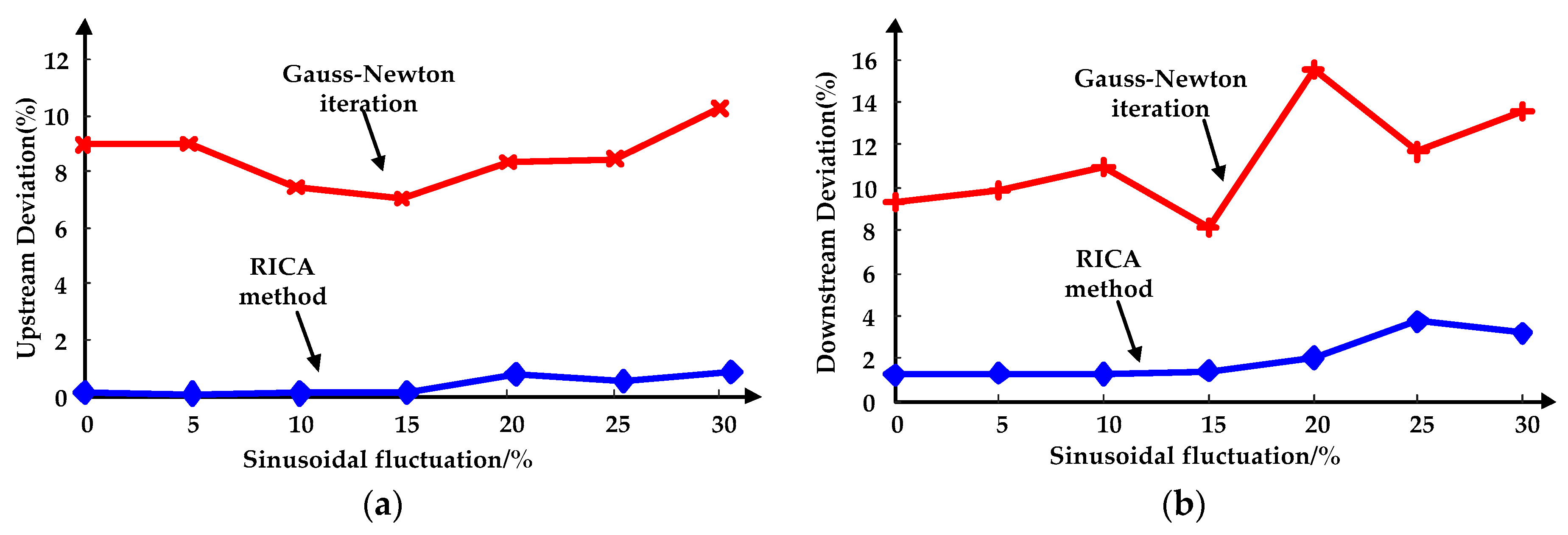
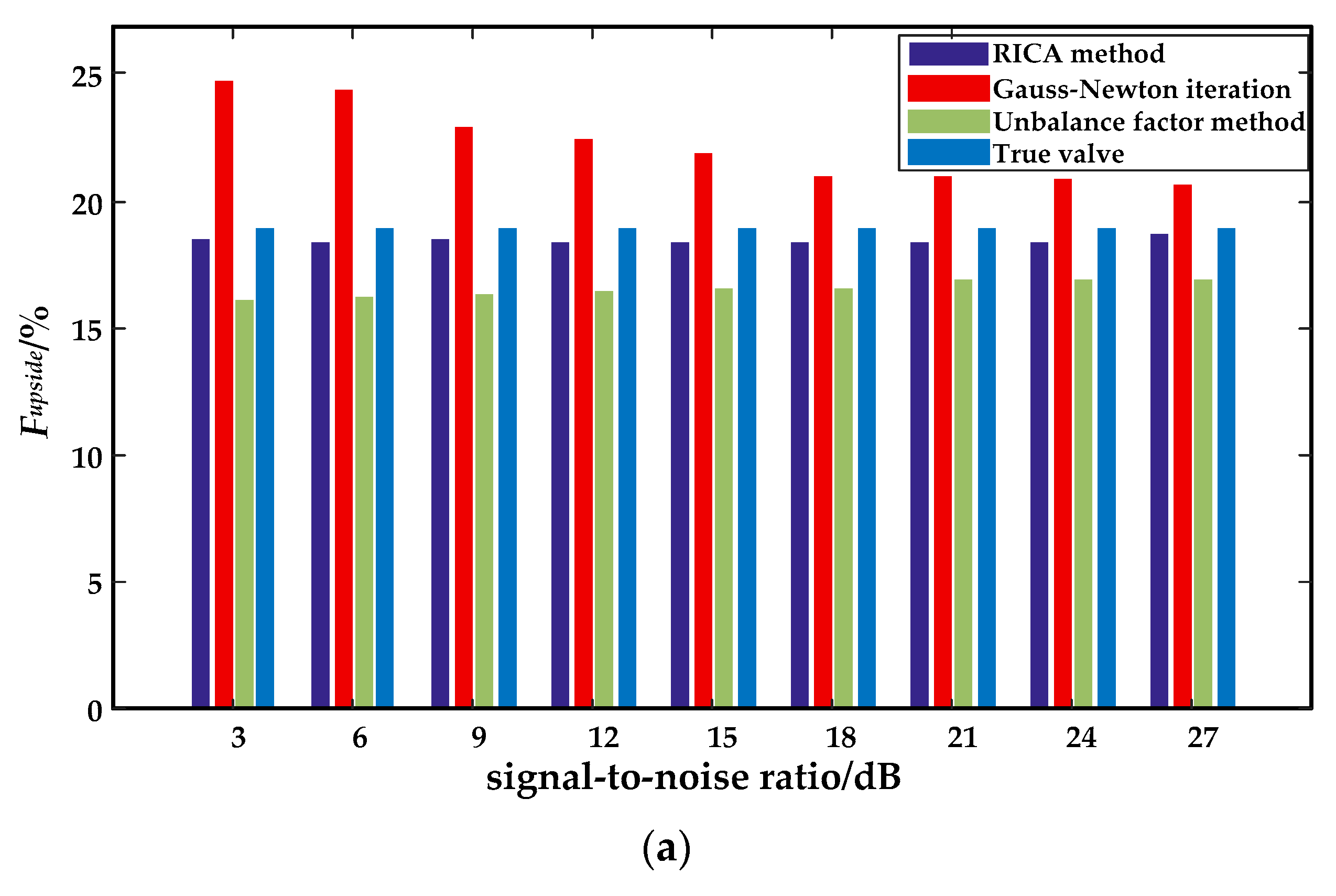
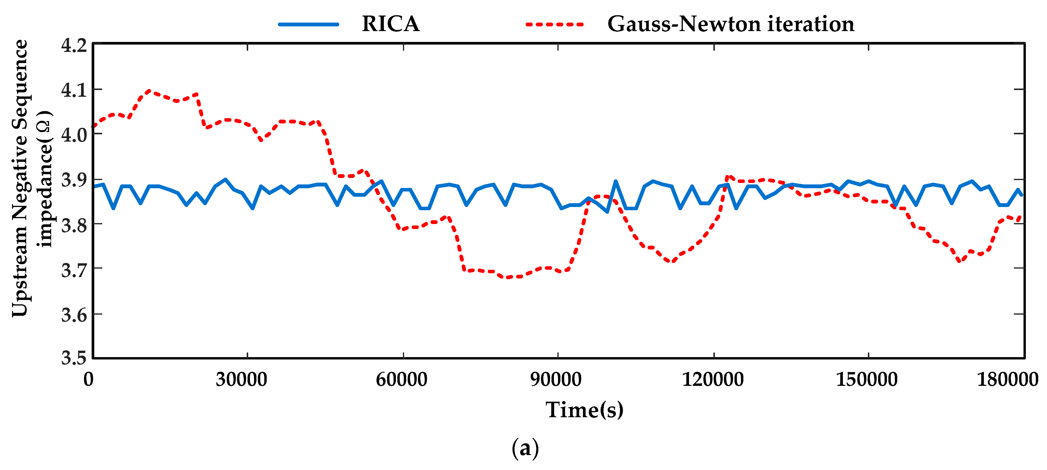
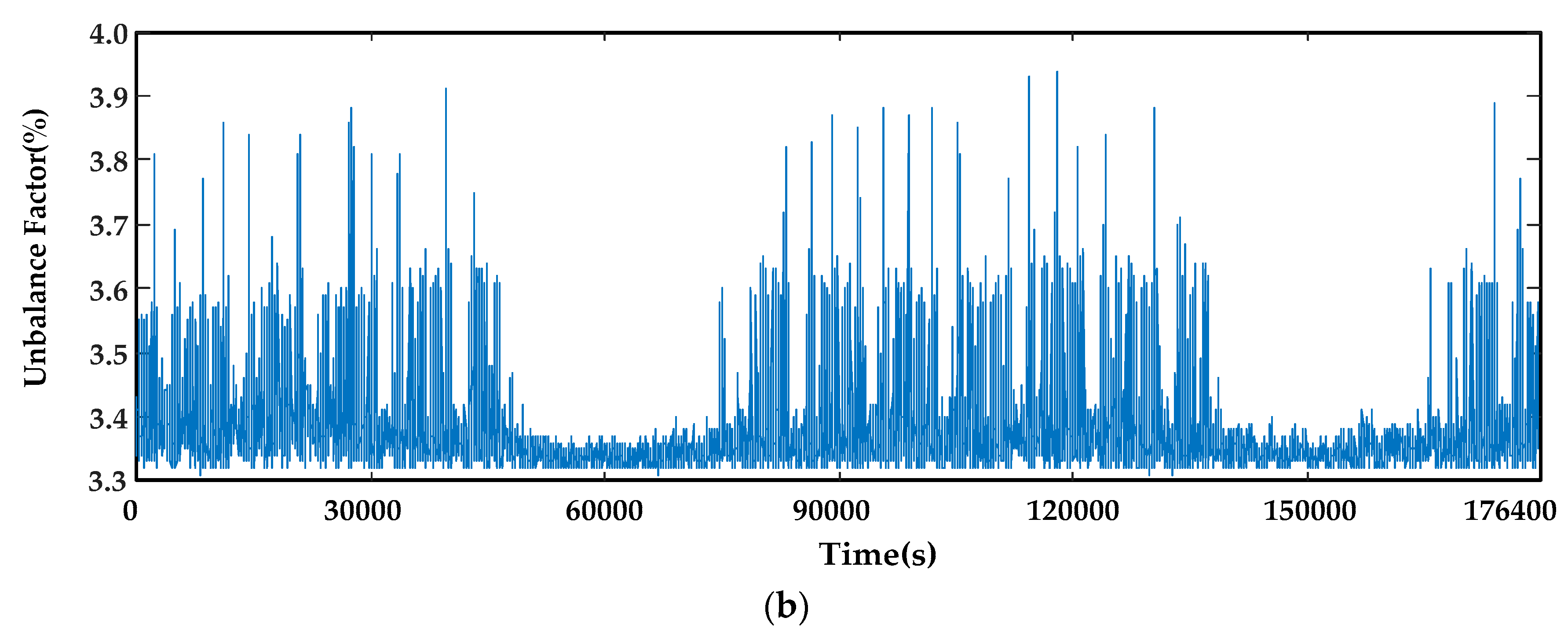
Through simulation analysis, the system impedance estimated by the method proposed in this paper was more accurate, and was closer to the true value than the traditional method. As the background noise and system fluctuations increased, the measurement error also increased, but the measurement error of the proposed method was much smaller than the traditional method and shows good anti-interference ability. When calculating the equivalent impedance and unbalance factor of the actual high-speed rail station, the equivalent impedance estimate was relatively stable, and the unbalance was in line with the actual situation. The division of responsibility for multiple unbalanced sources is the research direction to explore. in the future.

References

1. Haoran, W.; Pooya, D.; Huai, W.; Dinesh, K.; Firuz, Z.; Frede, B. Lifetime estimation of dc-link capacitors in adjustable speed drives under grid voltage unbalances. IEEE Trans. Power Electron. 2018, 34, 4064–4078. [Google Scholar]
2. Safa, A.; Berkouk, E.M.; Messlem, Y.; Gouichiche, A. A robust control algorithm for a multifunctional grid tied inverter to enhance the power quality of a microgrid under unbalanced conditions. Int. J. Electr. Power Energy Syst. 2018, 100, 253–264. [Google Scholar] [CrossRef]
3. Jayatunga, U.; Ciufo, P.; Perera, S.; Agalgaonkar, A.P.; Ciufo, P. Deterministic methodologies for the quantification of voltage unbalance propagation in radial and interconnected networks. IET Gener. Transm. Distrib. 2015, 9, 1069–1076. [Google Scholar] [CrossRef] [Green Version]
4. Abasi, M.; Seifossadat, S.G.; Razaz, M.; Moosapour, S.S. Determining the contribution of different effective factors to individual voltage unbalance emission in n-bus radial power systems. Int. J. Electr. Power Energy Syst. 2018, 94, 393–404. [Google Scholar] [CrossRef]
5. Sun, Y.; Li, P.; Li, S.; Zhang, L. Contribution Determination for Multiple Unbalanced Sources at the Point of Common Coupling. Energies 2017, 10, 171. [Google Scholar] [CrossRef]
6. Sun, Y.; Xie, X.; Li, P. Unbalanced source identification at the point of evaluation in the distribution power systems. Int. Trans. Electr. Energy Syst. 2018, 28, e2460. [Google Scholar] [CrossRef]
7. Electromagnetic Compatibility (EMC). Assessment of Emission Limits for the Connection of Unbalanced Installations to MV, HV and EHV Power Systems; TR 61000-3-13:2008; International Electrotechnical Commission (IEC): Geneva, Switzerland, 2008; pp. 3–13. [Google Scholar]
8. Seiphetlho, T.; Rens, A. On the assessment of voltage unbalance. In Proceedings of the 14th International Conference Harmonics Quality Power, Bergamo, Italy, 26–29 September 2010. [Google Scholar]
9. Lacerda Arao, L.; Ferreira Filho, A.; Borges Mendonca, M. Comparative Evaluation of Methods for Attributing Responsibilities Due To Voltage Unbalance. IEEE Trans. Power Deliv. 2016, 31, 743–752. [Google Scholar] [CrossRef]
10. Liu, Z.; Milanovic, J.V. Probabilistic Estimation of Voltage Unbalance in MV Distribution Networks with Unbalanced Load. IEEE Trans. Power Deliv. 2015, 30, 693–703. [Google Scholar] [CrossRef]
11. Wen, H.; Cheng, D.; Teng, Z.; Guo, S.; Li, F. Approximate Algorithm for Fast Calculating Voltage Unbalance Factor of Three-Phase Power System. IEEE Trans. Ind. Inform. 2014, 10, 1799–1805. [Google Scholar] [CrossRef]
12. Jayatunga, U.; Perera, S.; Ciufo, P.; Agalgaonkar, A.P. Voltage Unbalance Emission Assessment in Interconnected Power Systems. IEEE Trans. Power Deliv. 2013, 28, 2383–2393. [Google Scholar] [CrossRef] [Green Version]
13. Jayatunga, U.; Perera, S.; Ciufo, P. Voltage Unbalance Emission Assessment in Radial Power Systems. IEEE Trans. Power Deliv. 2012, 27, 1653–1661. [Google Scholar] [CrossRef]
14. Ghijselen, J.; Van Den Bossche, A. Exact voltage unbalance assessment without phase measurements. IEEE Trans. Power Syst. 2015, 20, 519–520. [Google Scholar] [CrossRef]
15. Gel/210/11. Voltage Characteristics of Electricity Supplied by Public Distribution Systems; British Standards Institution: London, UK, 1995. [Google Scholar]
16. Zarzoso, V.; Comon, P. Robust Independent Component Analysis by Iterative Maximization of the Kurtosis Contrast with Algebraic Optimal Step Size. IEEE Trans. Neural Netw. 2010, 21, 248–261. [Google Scholar] [CrossRef] [PubMed]
17. Hyvarinen, A. Fast and robust fixed-point algorithms for independent component analysis. IEEE Trans. Neural Netw. 1999, 10, 626–634. [Google Scholar] [CrossRef] [PubMed] [Green Version]
18. Beckmann, C.F.; DeLuca, M.; Devlin, J.T.; Smith, S.M. Investigations into resting-state connectivity using independent component analysis. Philos. Trans. R. Soc. B Boil. Sci. 2005, 360, 1001–1013. [Google Scholar] [CrossRef] [PubMed] [Green Version]
19. Bach, F.; Jordan, M. Kernel independent component analysis. J. Mach. Learn. Res. 2003, 3, 1–48. [Google Scholar]
20. Pruim, R.H.R.; Mennes, M.; van Rooij, D.; Llera, A.; Buitelaar, J.K.; Beckmann, C.F. ICA-AROMA: A robust ICA-based strategy for removing motion artifacts from fMRI data. NeuroImage 2015, 112, 267–277. [Google Scholar] [CrossRef]
21. Wang, T.; Liu, Y.; Sun, Y.; Li, P. Disturbance source locating for three-phase imbalance. Power Autom. Equip. 2015, 35, 43–48. [Google Scholar]
22. Hong, Y.-Y.; Wang, F.-M.; Wang, M.-D. Impact of high-speed railway loads on a longitudinal power system. IEE Proc. Electr. Power Appl. 1998, 145, 261. [Google Scholar] [CrossRef]
23. Kuo, H.-Y.; Chen, T.-H. Rigorous evaluation of the voltage unbalance due to high-speed railway demands. IEEE Trans. Veh. Technol. 1998, 47, 1385–1389. [Google Scholar]
24. Kao, F.-C.; Chen, S. Specification of minimum short-circuit capacity for three-phase unbalance limitation based on an efficient algorithm. Electr. Power Syst. Res. 1996, 39, 223–232. [Google Scholar] [CrossRef]
Figure 1. The typical system circuit. PCC: point of common coupling.
Energies 12 02849 g001
Figure 2. Norton equivalent circuit of upstream and downstream.
Energies 12 02849 g002
Figure 3. Negative-sequence voltage vector relationship diagram.
Energies 12 02849 g003
Figure 4. Three-phase unbalanced source responsibility division flowchart based on robust independent component analysis (RICA).
Energies 12 02849 g004
Figure 5. Simulation system diagram.
Energies 12 02849 g005
Figure 6. Fifty upstream equivalent–impedance calculations resulting from two methods: (a) 50 upstream equivalent–impedance calculations resulting from the RICA method; (b) 50 upstream equivalent–impedance calculations result from the Gauss–Newton iteration method.
Energies 12 02849 g006
Figure 7. The execution times of (a) the RICA method, and (b) the Gauss–Newton iteration method.
Energies 12 02849 g007
Figure 8. Relationship between equivalent impedance and load unbalance factor: (a) relationship between upstream equivalent impedance and load unbalance factor; (b) relationship between downstream equivalent impedance and load unbalance factor.
Energies 12 02849 g008
Figure 9. The calculation results of the upstream and downstream unbalance source contribution by three methods: (a) the contribution of upstream and downstream unbalance sources; (b) the contribution deviation of the upstream and downstream for the three methods.
Energies 12 02849 g009
Figure 10. Relationship between the equivalent-impedance calculation and the sinusoidal fluctuation of the system parameters: (a) relationship between upstream impedance deviation and the sinusoidal fluctuation of the system; (b) relationship between downstream impedance deviation and the sinusoidal fluctuation of the system.
Energies 12 02849 g010
Figure 11. Comparison of the contribution of the upstream unbalance source and the signal-to-noise ratio: (a) relationship between the signal-to-noise ratio and the contribution of the upstream; (b) relationship between the signal-to-noise ratio and the deviation.
Energies 12 02849 g011aEnergies 12 02849 g011b
Figure 12. Unbalance parameter at each moment of the traction substation: (a) downstream negative-sequence impedance at each moment; (b) unbalance factor at each moment.
Energies 12 02849 g012aEnergies 12 02849 g012b